i

Methods for Reconstruction of Transient Emissions from

Heavy-Duty Vehicles

Madhava R. Madireddy

Dissertation submitted to the

College of Engineering and Mineral Resources

at West Virginia University

in partial fulfillment of the requirements

for the degree of

Doctor of Philosophy

in

Mechanical Engineering

Committee Members:

Nigel N. Clark, Ph.D., Chair

Eric K. Johnson, Ph.D.

Jacky C. Prucz, Ph.D.

Natalia A. Schmid, Ph.D.

W. Scott Wayne, Ph.D.

Department of Mechanical and Aerospace Engineering

Morgantown, WV

2008

Keywords: Dispersion Function, Reconstruction of Emissions, Engine

Dynamometer, Instantaneous Emissions, Deconvolution

ii

ABSTRACT

Methods for Reconstruction of Transient Emissions from

Heavy-Duty Vehicles

Madhava R. Madireddy

Emissions measurement analyzers give out a response that may not reflect the true

instantaneous engine-out emissions. Currently, the heavy-duty diesel engines are being

certified for emissions measured in a thirty second time window with certain

specification requirements for the analyzers. Since these measured emissions values may

not be the same as the true instantaneous emissions, integrated values for the thirty

second windows may be affected by analyzer response.

This document presents and examines reconstruction techniques to estimate

instantaneous heavy-duty engine-out emissions. These techniques will take as the input,

the continuous set of emissions data and approximate dispersion characteristics of the

analyzer employed in measuring the continuous data. For this purpose, this research dealt

with understanding and modeling the transient dynamics (dispersion function) of the

analyzers and the sampling system to establish a relationship between the measured and

instantaneous heavy-duty emissions.

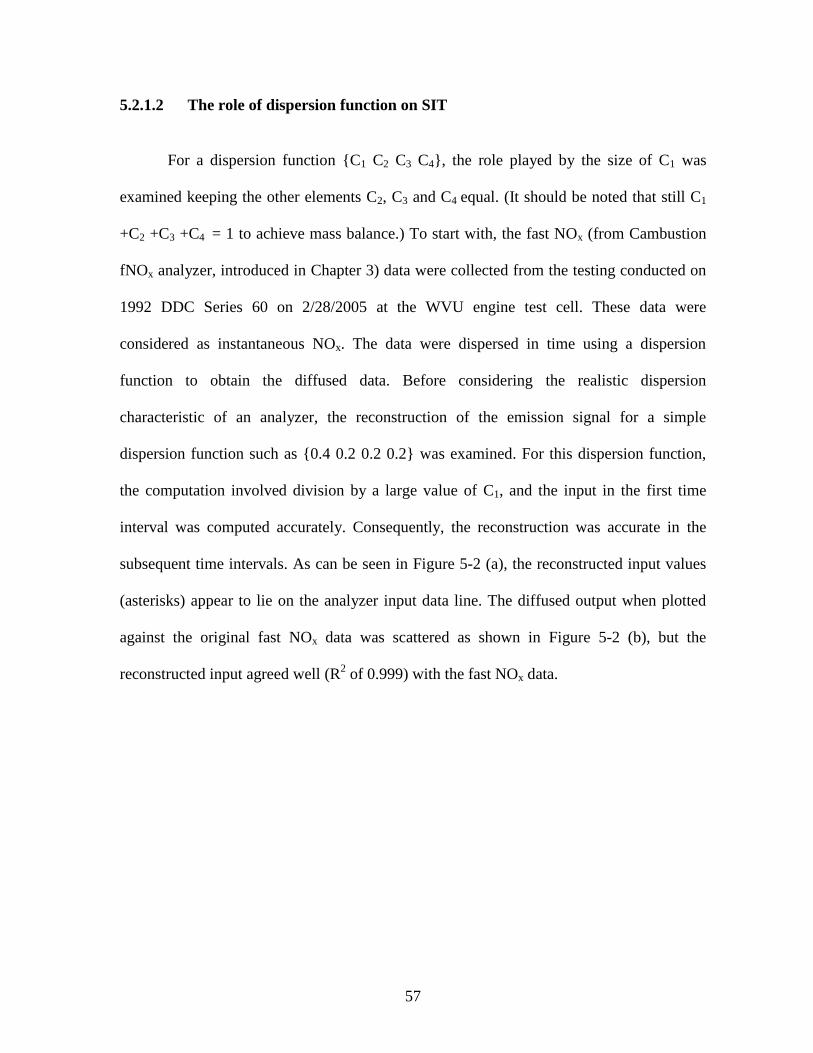
Four methods of reconstruction were presented in this study: Sequential Inversion

Technique (SIT), Differential Coefficients Method (DCM), Inverse Fast Fourier

Transform (IFFT) and Modified Deconvolution Technique (MDT). The application of

each method in reconstructing real-time emissions data was presented. While SIT failed

in practical applications, each of the other three methods was shown to offer advantage in

the post-processing of the measured emissions data. DCM accounted for the small errors

iii

in the computation of the analyzer dispersion function. IFFT was able to reconstruct just

as well as DCM; however the Fast Fourier Transform of the dispersion function should

be high enough to ensure stability of the method. In other words, the dispersion function

should not have elements that were almost equal to zero for the method to be stable. Both

the DCM and IFFT improved the correlation of emissions with power by an average of

about 2%. MDT employs fitting a gamma distribution to the dispersion function and

searches for the best possible distribution within a prescribed range to improve the

reconstruction. With emissions reconstruction using MDT, the improvement of

correlation of emissions with power was approximately about 3%.

The measured continuous data of CO2 mass flow rate from the New Flyer 2006

transit bus was divided into several operating bins, each bin having a specific speed and

acceleration range. MDT was used to generate continuous reconstructed emissions from

the measured continuous data. This reconstructed data is again divided into identical bins

following a similar procedure. By comparing the two sets of bins, it was found that at low

accelerations, the average mass flow rate of the measured CO2 was lesser than that of the

reconstructed CO2. However, the reverse was found true at high accelerations.

This work could enhance the existing inventory models, help the calibrators

appreciate the affect of time dispersion and can take the certifiers one step closer to

estimating the true transient emissions by compensating for the distortion of the

measurement systems.

iv

ACKNOWLEDGEMENTS

I am extremely grateful to my advisor Dr. Nigel Clark. He has been a great support for

me throughout my doctorate program. I am glad I had an opportunity to work under his

guidance to obtain the highest degree in my career. I would like to thank Dr. Eric

Johnson, Dr. Jacky Prucz, Dr. Natalia Schmid, and Dr. Scott Wayne for being my

committee members and for their suggestions.

I want to express my sincere gratitude to everyone who worked at the EERC at WVU

who have helped me during the research work. Firstly, I need to thank Richard Atkinson,

who helped me repair the Fast NOx analyzer and Bradley Ralston who helped me collect

data for different runs. I would like to thank Ajtay and Weilenmann, since I applied a

theory suggested by them in this dissertation. I also thank Matthew Spears of the EPA for

drawing my attention to their work. I would like to thank Lijuan for collaborating with

me in some of my data analysis. I would also like to specially thank Xiaohan Chen and

Nikhil Burri for providing me invaluable help in understanding and applying signal

processing in my data analysis. I would like to thank my colleagues Kevin Flaim, Major

Khan, Emre, Kuntal, Clinton and Lijuan for their cooperation. Next I would like to thank

Mimi Roy and my wife, Greeshma for her editing help. I am very grateful to my family

who had been supportive of me pursuing a doctoral degree. I dedicate my dissertation to

them. Finally, I would like to thank the Department of Transportation (contract number

10009291.1.1.1003596R) for their continual sponsorship for this study.

v

TABLE OF CONTENTS

1 INTRODUCTION, OVERVIEW & OBJECTIVES ........................................................................ 1

1.1 INTRODUCTION............................................................................................................................. 1 1.2 OVERVIEW ................................................................................................................................... 1 1.3 PURPOSE AND OBJECTIVE OF THE RESEARCH ................................................................................ 2 1.4 PLAN TO MEET THE OBJECTIVE ..................................................................................................... 3 1.5 ORGANIZATION OF THIS DOCUMENT............................................................................................. 3

2 LITERATURE REVIEW................................................................................................................... 5

2.1 AIR QUALITY AND HEALTH EFFECTS OF EMISSIONS ...................................................................... 5 2.2 SIGNIFICANCE OF HEAVY-DUTY EMISSIONS .................................................................................. 6 2.3 HEAVY-DUTY CYCLE DEVELOPMENT ........................................................................................... 6 2.4 UNITS FOR MEASUREMENT OF HEAVY-DUTY EMISSIONS .............................................................. 8 2.5 STEADY STATE AND TRANSIENT EMISSIONS TEST CYCLES ............................................................ 9 2.6 NEED FOR CONTINUOUS DATA OF EMISSIONS ............................................................................... 9 2.7 HEAVY-DUTY EMISSIONS STANDARDS.........................................................................................10 2.8 CONSENT DECREES ......................................................................................................................12 2.9 THE SET LIMITS ..........................................................................................................................12 2.10. NTE LIMITS .................................................................................................................................13 2.11 DEFINITION AND REQUIREMENTS OF THE NTE EVENT .................................................................14 2.12 PROBLEMS WITH NTE OPERATION ..............................................................................................15 2.13 NTE WINDOW SIZE .....................................................................................................................16 2.14 MOTIVATION TO IMPROVE MEASUREMENT ACCURACY ...............................................................16 2.15 ON BOARD MEASUREMENT ..........................................................................................................17 2.16 EMISSION INVENTORY MODELS ...................................................................................................18

2.16.1 Traffic situation models ....................................................................................................19 2.16.2 Average speed model ........................................................................................................20 2.16.3 Physical models ................................................................................................................20 2.16.4 Modal emissions model .....................................................................................................20 2.16.5 Instantaneous emissions models .......................................................................................21

3 THEORY OF DELAY AND DISPERSION OF DATA .................................................................22

3.1 MEASUREMENT AND COMPENSATION OF DELAY .........................................................................22 3.1.1 Measurement delay ................................................................................................................22 3.1.2 Compensation for delay and brief review of literature ..........................................................23

3.2 TIME DISPERSION OF DATA AND EARLIER WORK RELATED TO DATA DISPERSION.........................24 3.2.1 Theory of dispersion ..............................................................................................................25 3.2.2 Earlier work related to dispersion of data .............................................................................26 3.2.3 Understanding the transient dynamics of the analyzers ........................................................27 3.2.4 Understanding the effects of dispersion on a step input ........................................................30 3.2.5 Emissions ‘lost’ in measurement due to dispersion ...............................................................31 3.2.6 The ‘gain’ of emissions that corresponds to the ‘loss’ of emissions ......................................34 3.2.7 Amplitude reduction due to dispersion of data ......................................................................35

4 EXPERIMENTAL EQUIPMENT, PROCEDURES AND AVAILABLE DATA ........................36

4.1 OPERATION OF THE ENGINE TEST CELL ........................................................................................36 4.2 ANALYZERS USED FOR EMISSIONS MEASUREMENT ......................................................................37

4.2.1 CO and CO2 analyzers...........................................................................................................38 4.2.2 HC analyzer ...........................................................................................................................39 4.2.3 Regular NOx analyzer ............................................................................................................39 4.2.4 Fast NOx analyzer ..................................................................................................................40

4.3 ENGINE DATA USED IN THE ANALYSIS .........................................................................................42 4.4 CHASSIS DYNAMOMETER TESTING PROCEDURE ...........................................................................44 4.5 CHASSIS DATA USED FOR ANALYSIS ............................................................................................45

vi

4.5.1 Vehicles tested on the chassis dynamometer .........................................................................45 4.5.2 Drive cycles used for the chassis dynamometer data ............................................................46

5 DATA ANALYSIS AND RESULTS ..................................................................................................50

5.1 APPLYING THE FORWARD TRANSFORM ............................................................................................50 5.1.1 Operating variables that can simulate instantaneous data ....................................................50 5.1.2 Applying the forward transform to axle power ......................................................................51 5.1.3 The effect of dispersion of axle power ....................................................................................52 5.1.4 Constraint on emissions data for back-transformation ..........................................................53 5.1.5 Assumptions for the analyzer system .....................................................................................53

5.2 INTRODUCTION AND APPLICATION OF BACK-TRANSFORMATION TECHNIQUES ..................................55 5.2.1 Sequential inversion technique (SIT) [96] .............................................................................56 5.2.1.1 Theory of SIT .......................................................................................................................56 5.2.1.2 The role of dispersion function on SIT ................................................................................57 5.2.2 Differential coefficients method (DCM) .................................................................................62 5.2.2.1 Definition and implementation of DCM ..............................................................................62 5.2.2.2 Validating DCM ..................................................................................................................63 5.2.2.2.1 Validating DCM in reconstructing NOx data ...................................................................63 5.2.2.2.2 Validating DCM in reconstructing CO2 data ...................................................................65 5.2.2.3 Improvement of DCM ..........................................................................................................68 5.2.2.3.1 Effect of forward, central and backward differences .......................................................68 5.2.2.3.2 Effect of multiple derivatives on DCM .............................................................................69 5.2.2.4 Stability of DCM ...........................................................................................................70 5.2.3 Fast Fourier Transform (FFT) and Inverse Fast Fourier Transform (IFFT) ........................71 5.2.3.1 Modeling the analyzer system .............................................................................................71 5.2.3.2 Theory of IFFT .................................................................................................................72 5.2.3.3 Illustrating and validating IFFT .........................................................................................74 5.2.3.4 Criterion for stability of IFFT .............................................................................................74 5.2.3.5 Comparing reconstruction ‘efficiency’ of IFFT and DCM .................................................77 5.2.3.5.1 IFFT vs. DCM for reconstructing CO2 ............................................................................77 5.2.3.5.2 IFFT vs. DCM for reconstructing NOx .............................................................................81 5.2.4 Modified deconvolution technique (MDT) .............................................................................84 5.2.4.1 Definition of blind-deconvolution .......................................................................................84 5.2.4.2 Reformulation of blind-deconvolution ................................................................................85 5.2.4.3 Theory and application of modified deconvolution technique (MDT) ................................86 5.2.4.3.1 Obtaining a priori information ........................................................................................86 5.2.4.3.2 Computation of approximate output ................................................................................87 5.2.4.3.3 Application of MDT for emission reconstruction .............................................................87 5.2.5 Influence of the operating condition on emission reconstruction ..........................................89 5.2.5.1 Processed data and drive cycles ......................................................................................89 5.2.5.2.1 Division of the data into bins ............................................................................................90 5.2.5.3 Average emissions in each bin .........................................................................................93 5.2.5.4 The standard deviation of emissions in each bin .............................................................96

6 CONCLUSIONS AND RECOMENDATIONS ...............................................................................98

6.1 SUMMARY OF THE RESEARCH ......................................................................................................98 6.2 CONCLUSIONS .............................................................................................................................99 6.3 RECOMMENDED THEME FOR HEAVY-DUTY EMISSIONS RECONSTRUCTION .................................100 6.4 APPLICATIONS OF THE RESEARCH WORK ...................................................................................101

6.4.1 Application in the field of inventory modeling .....................................................................101 6.4.2 Application of reconstruction for data analysts ...................................................................101 6.4.3 Application in the field of engine certification by EPA .......................................................102

6.5 RECOMMENDATIONS FOR FUTURE WORK ..................................................................................102

REFERENCES ..........................................................................................................................................104

vii

LIST OF FIGURES

Figure 2-1. FTP Transient Cycle ....................................................................................... .8

Figure 2-2. NTE torque and speed boundaries ................................................................ 14

Figure 3-1 (a). Impulse response of Rosemount 955 NOx analyzer ................................. 29

Figure 3-1 (b). Impulse response of Horiba AIA 210 analyzer ........................................ 30

Figure 3-2. The effect of dispersion on a step input ......................................................... 31

Figure 3-3. The effect of dispersion on a 30-second rectangular wave ............................ 32

Figure 3-4. The effect of dispersion on a 10 second rectangular wave ............................ 33

Figure 3-5. Percent of lost emissions as a function of window size ................................. 34

Figure 3-6. Amplitude reduction due to dispersion of data .............................................. 35

Figure 4-1. Emissions bench at WVU-engine test cell ..................................................... 37

Figure 4-2 (a). Fast NOx sampling unit ............................................................................. 40

Figure 4-2 (b). Remote Sampling head of Fast NOx mounted on the dilution tunnel ...... 41

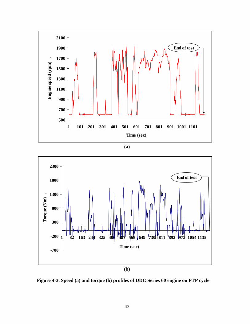
Figure 4-3. Speed (a) and torque (b) profiles of DDC Series 60 engine on FTP

drive cycle ......................................................................................................................... 43

Figure 4-4. Speed profiles of different modes of HHDDT drive cycle ............................ 48

Figure 4-5. Speed profile of UDDS drive cycle ............................................................... 49

Figure 5-1. The effect of dispersion on the correlation between emission rate and

axle power ......................................................................................................................... 52

Figure 5-2 (a). Illustration of the time-invariance of a system…………………………………..……..54

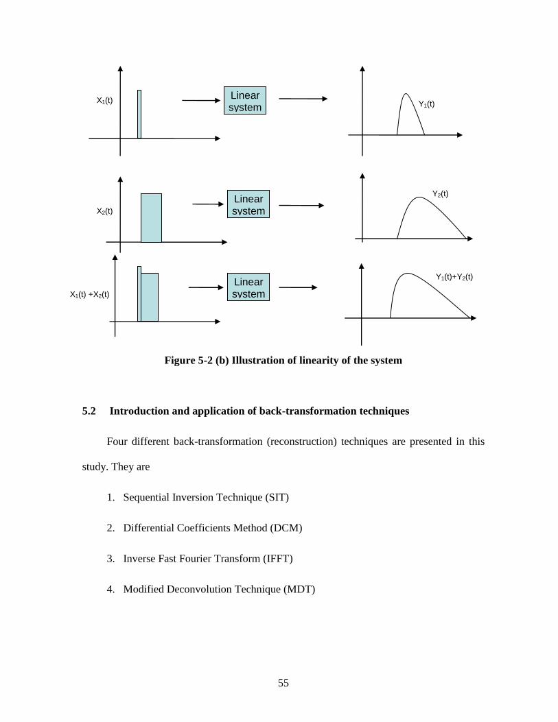
Figure 5-2 (b). Illustration of the linearity of a system……………..……..……...…..……..…….….……55

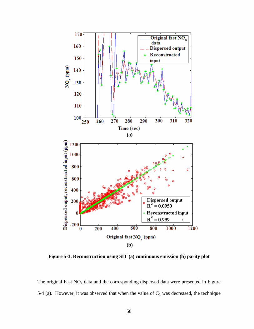
Figure 5-3. Reconstruction using SIT (a) continuous emission (b) parity plot ................ 58

Figure 5-4. SIT applied to a NOx analyzer………… ....................................................... 60

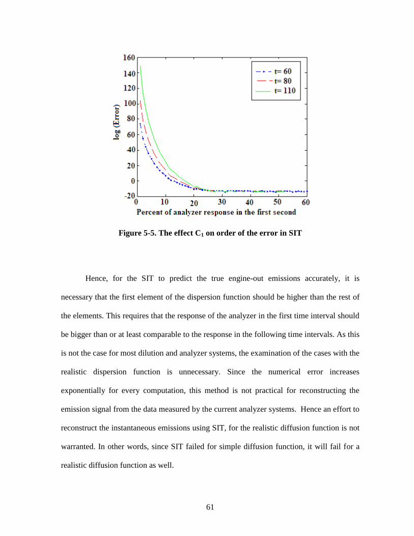
Figure 5-5. The effect C1 on order of the error in SIT ..................................................... 61

Figure 5-6. NOx reconstruction using DCM (a & b) Continuous data (c) Parity plot ...... 65

Figure 5-7. CO2 reconstruction using DCM (a) Parity plot (b) Continuous data.............. 67

Figure 5-8. Representation of the system in time domain ................................................ 72

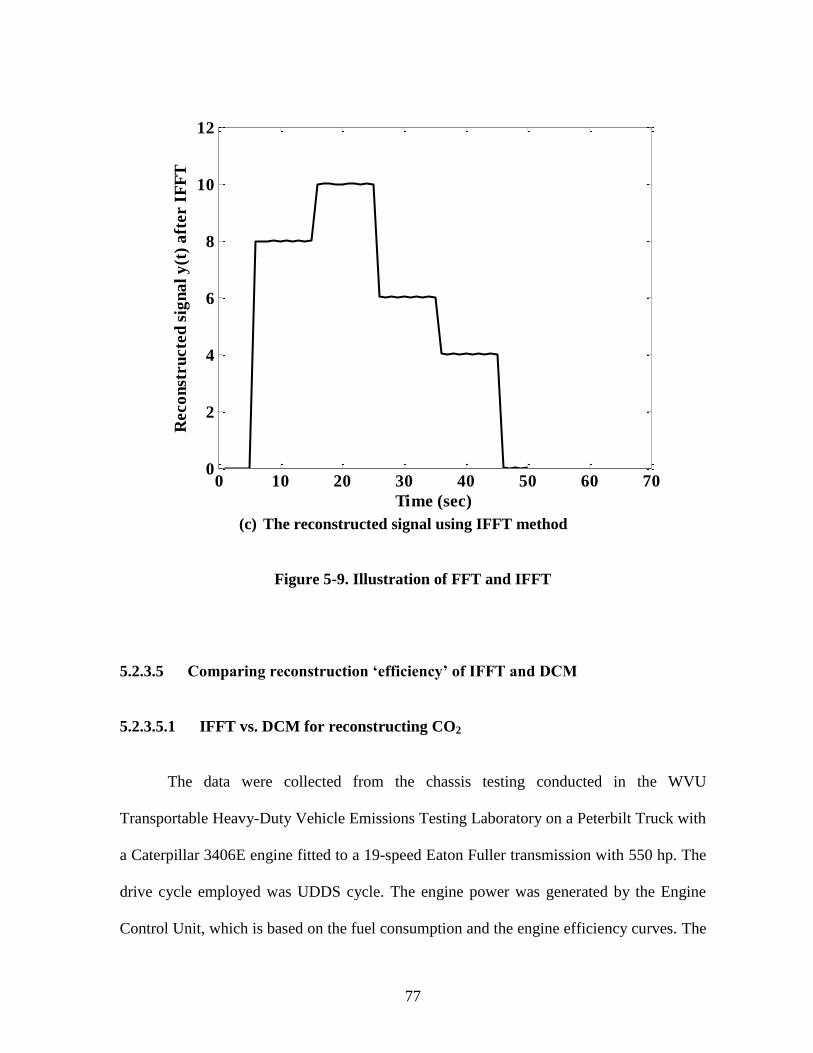
Figure 5-9. Illustration of FFT and IFFT .......................................................................... 77

Figure 5-10. Comparison of DCM and IFFT in reconstruction of CO2 emissions from

Peterbilt truck with Caterpillar 3406E engine tested on TEST_D cycle .......................... 80

Figure 5-11. Comparison of DCM and IFFT in reconstruction of NOx emissions from

Peterbilt truck with Caterpillar 3406E engine tested on UDDS cycle .............................. 83

Figure 5-12. Fitting a gamma distribution to the dispersion function .............................. 86

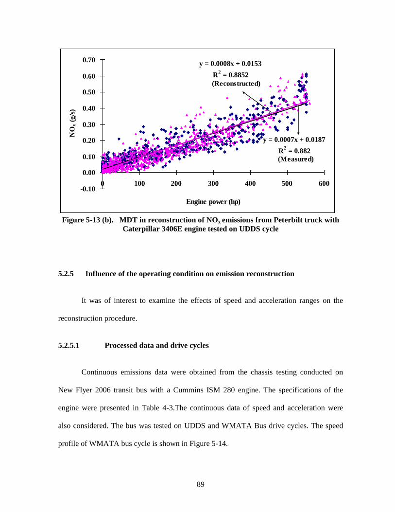
Figure 5-13 (a). MDT in reconstruction of CO2 emissions from Peterbilt truck with

Caterpillar 3406E engine tested on UDDS cycle ............................................................. 88

Figure 5-13 (b). MDT in reconstruction of NOx emissions from Peterbilt truck with

Caterpillar 3406E engine tested on UDDS cycle ............................................................. 89

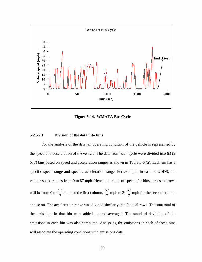
Figure 5-14. WMATA Bus Cycle.…………….…......................………….………….………………....90

Figure 5-15 (a). The ratio of bin average of the reconstructed to measured emissions

for New Flyer 2006 Transit bus tested on UDDS drive cycle…………………..……......94

Figure 5-15 (b). The ratio of bin average of the reconstructed to measured emissions

for New Flyer 2006 Transit bus tested on WMATA drive cycle……………..…...……........…..…...94

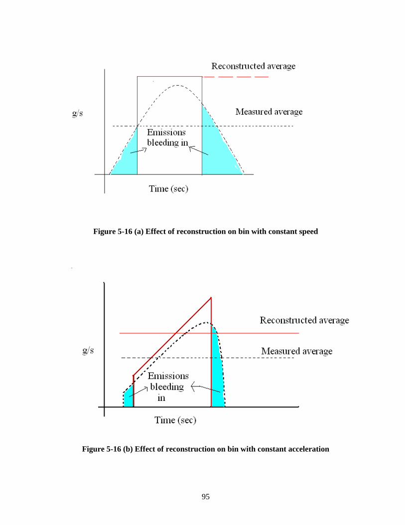
Figure 5-16 (a). Effect of reconstruction on bin with constant speed…………………..…..………95

Figure 5-16 (b). Effect of reconstruction on bin with constant acceleration........………95

viii

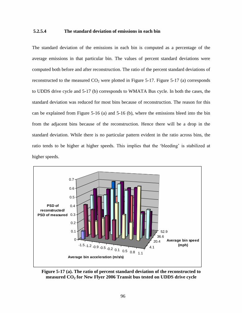
Figure 5-17 (a). The ratio of percent standard deviation of the reconstructed

to measured emissions for New Flyer 2006 Transit bus tested on UDDS drive

cycle………………………………………………………………………….……….....96

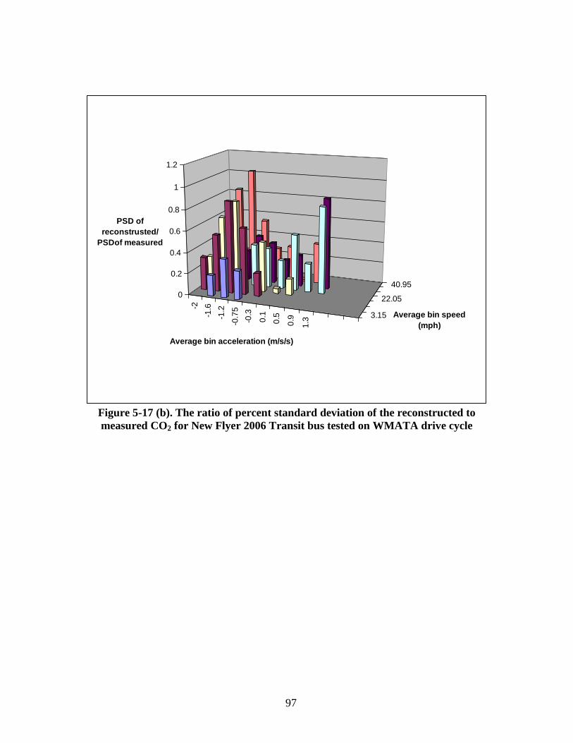
Figure 5-17 (b). The ratio of percent standard deviation of the reconstructed to

measured emissions for New Flyer 2006 Transit bus tested on WMATA drive

cycle……………………………………………………………………………………..97

ix

LIST OF TABLES

Table 2-1. Emission standards for heavy duty diesel engines ......................................... 11

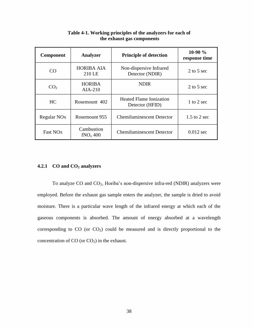
Table 4-1. Working principles of the analyzers for each of the exhaust gas

components……………………………………………………………………………………………………………………….38

Table 4-2. Details of the engines tested on the engine dynamometer .............................. 42

Table 4-3. Details of the vehicles tested……………. ...................................................... 46

Table 5-1. R2 values for the three FTP runs examined to test the validity of the DCM ... 65

Table 5-2. Errors in DCM with different numerical methods for computing the

derivatives ......................................................................................................................... 67

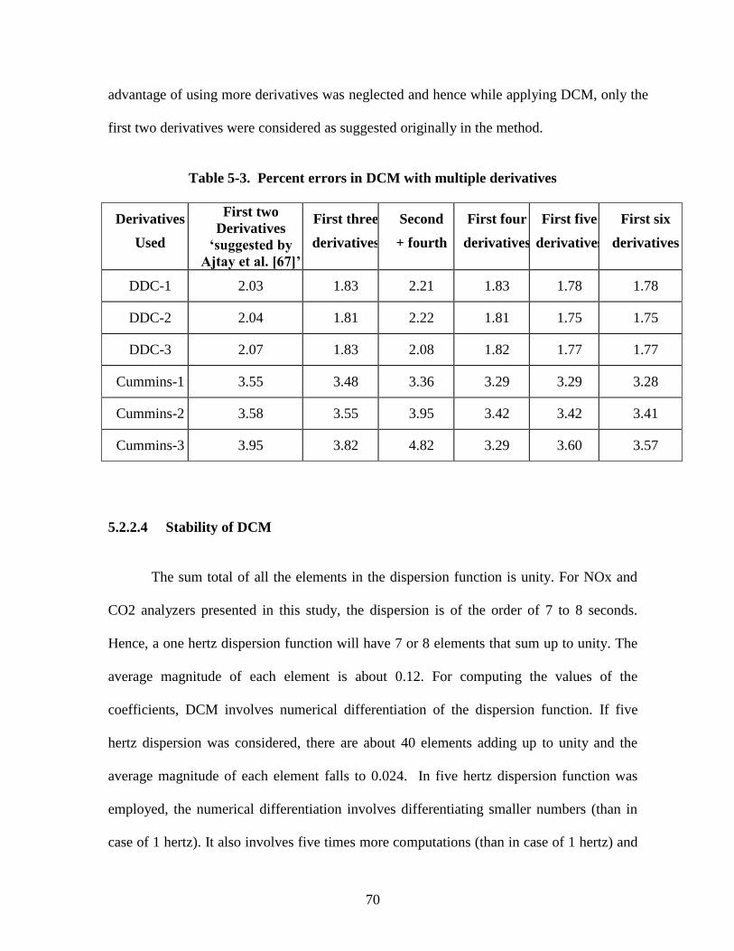
Table 5-3. Errors in DCM with multiple derivatives ....................................................... 69

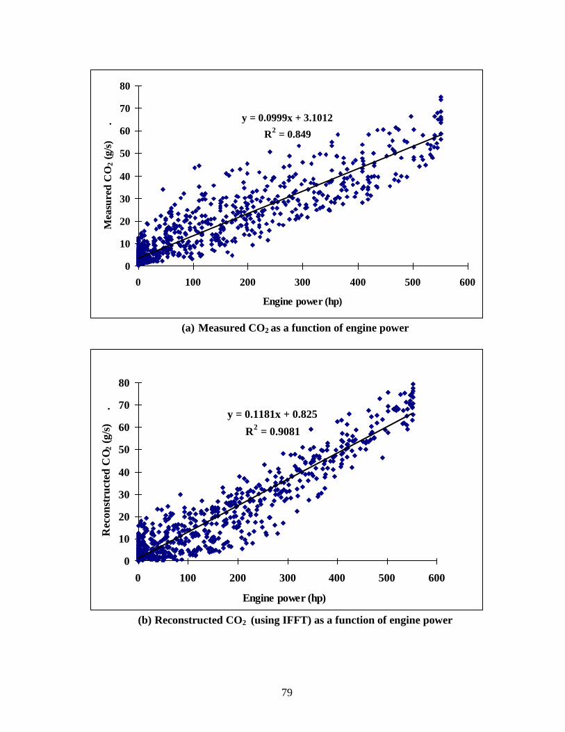
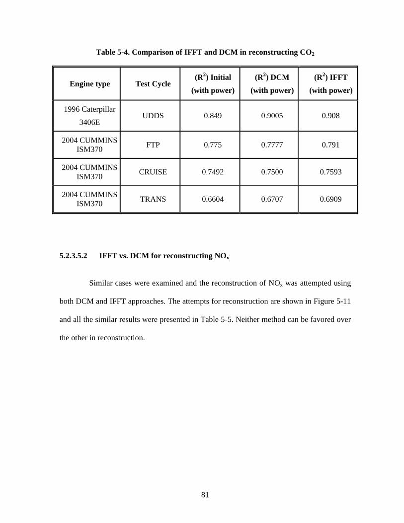
Table 5-4. Comparison of IFFT and DCM in reconstructing CO2 ................................... 81

Table 5-5. Comparison of DCM and IFFT in reconstructing NOX .................................. 84

Table 5-6 (a). Measured CO2 (g/s) for different combinations of speed and

acceleration from a New Flyer 2006 Transit bus tested on UDDS drive

cycle...................................................................................................................................91

Table 5-6 (b) Reconstructed CO2 (g/s) for different combinations of speed and

acceleration from a New Flyer 2006 Transit bus tested on WMATA drive

cycle……….……………………………………………………………………………..92

x

NOMENCLATURE AND ABBREVIATIONS

∆t Time shift

∆tav Average time shift

∏ Correlation Coefficient

bsfc Brake-Specific Fuel Consumption

0C Degree Celsius

Ci Ith

element of the dispersion function

C(t) Emission rate

CARB California Air Resources Board

CAT Caterpillar

CFR Code of Federal Regulations

CO Carbon Monoxide

CO2 Carbon Dioxide

COPERT Computer Program to Calculate Emissions from Road Transport

CRC Coordinating Research Council

D Axial dispersion coefficient

d Coefficient of molecular dispersion

D/uL Vessel dispersion number

DCM Differential Coefficients Method

DDC Detroit Diesel Corporation

DOT Department of Transportation

ECT Engine Coolant Temperature

ECU Engine Control Unit

EERL Engine and Emissions Research Laboratory

EGR Exhaust Gas Recirculation

EPA Environmental Protection Agency

ESC European Stationary Cycle

Ej Emission at time t=tj

0F Degree Fahrenheit

FFT Fast Fourier Transform

fNOx Fast NOx

FTIR Fourier Transform Infrared

xi

FTP Federal Test Procedure

g/bhp-hr Grams per brake horsepower hour

g/mile Grams per mile

g/sec Grams per second

gal Gallon

GVWR Gross Vehicle Weight Rating

H Dispersion function

HC Hydrocarbons

HDDE Heavy-Duty Diesel Engine

HHDDT Heavy Heavy-Duty Diesel Truck

hm Transfer function

hp Horsepower

Hz Hertz

IFFT Inverse Fast Fourier Transform

IMP Inlet Manifold Pressure

IMT Inlet Manifold Temperature

K,θ parameters of the gamma distribution

kg Kilograms

km Kilometer

kW Kilowatts

lb Pounds

lb-ft Foot-pound

MDT Modified De-convolution Technique

MEMS Mobile Emissions Measurement System

MEP Mean Effective Pressure

mph Miles per hour

m/s Meters per second

m/s2

Meters per second squared

MVEI Motor Vehicle Emission Inventory

N Size of the continuous data

NDIR Non-Dispersive Infrared

NMHC Non-Methane Hydrocarbons

NO Nitric Oxide

xii

NO2 Nitrogen dioxide

NOX Oxides of nitrogen

NTE Not-To-Exceed

PEMS Portable Emissions Measurement System

PM Particulate Matter

ppm Parts Per Million

PREVIEW Portable Real-Time Emission Vehicular Integrated Engineering

Workstation

PSF Point Spread Function

Pi Power at time t=i

R2

Coefficient of regression

ROVER Real-time On-road Vehicle Emissions Recorder

RPM Revolutions per Minute

SAE Society of Automotive Engineers

SET Supplemental Emissions Test

SIT Sequential Inversion Technique

std standard deviation

t Time

θi Non dimensional time

TRANS-LAB Transportable Laboratory

UDDS Urban Dynamometer Driving Schedule Chassis Dynamometer Cycle

U(ti) Analyzer input at time t=i

US EPA United States Environmental Protection Agency

UV Ultra-Violet

VGT Variable Geometry Turbocharger

WMATA Washington Metropolitan Area Transit Authority

WVU West Virginia University

x(t) Analyzer input

Y(ti) Analyzer output at time t=i

Y/(t)

First time derivative of the analyzer output

Y//(t)

Second time derivative of the analyzer output

1

1 Introduction, Overview & Objectives

1.1 Introduction

Internal Combustion (IC) engines produce exhaust that contains carbon monoxide

(CO), nitrogen oxides (NOx), hydrocarbons (HC) and particulate matter (PM). These

emissions deteriorate the quality of the atmospheric air and human health. The United

States Environmental Protection Agency (USEPA) introduced Clean Air Act in 1963 and

ever since the emissions have been regulated.

In spite of their high initial cost and cold start problems, diesel engines are a

popular, if not, automatic choice in heavy-duty trucks mainly because of their fuel

efficiency. In order to further improve fuel efficiency and reduce emissions, most of the on-

road, heavy-duty trucks in the United States are equipped with direct injection diesel

engines which are turbocharged and electronically controlled. The emissions from the

diesel engine vary significantly from those from a gasoline engine. Particularly, NOx

concentrations are much higher from diesel engines than from gasoline engines. NOx is a

major contributor to photochemical smog, acid rain and low level ozone formation.

1.2 Overview

„Instantaneous‟ emissions are the actual emissions produced by the engine due to

the combustion of the fuel. A measurement system can be used to record these

instantaneous emissions, but the system will distort the signal that corresponds to the

instantaneous emissions and produce an output signal, which represents the „measured‟

emissions. For an ideal analyzer system, the measured emissions will be the same as the

2

instantaneous emissions. However, any real analyzer system will report a distorted signal

during the process of measurement. For example, the emissions reported by the analyzer

may be delayed and dispersed relative to the instantaneous emissions.

By understanding the relationship between the measured and the instantaneous

emissions, an attempt can be made to obtain the instantaneous signal from the measured

signal. This procedure will be referred to as „reconstruction‟ in this document. Transient

dynamics of the analyzer need to be measured and understood through laboratory

procedures. This enables verifying the accuracy of the reconstruction that can be applied to

the measured data.

1.3 Purpose and objective of the research

EPA currently certifies engines for emissions in a thirty second NTE (Not-To-

Exceed) window. This involves driving the vehicle continuously for at least 30 seconds

within the operating constraints associated with NTE certification. A more detailed

description of the certification procedure is given in Chapter 2 and the effects of the

window size are discussed in Chapter 3. Currently, the measured emissions are regulated

and the analyzer systems must meet a specification. But the emissions that are measured

are not in fact the true (instantaneous) emissions. Since the measurement systems distort

the true emissions, there is a chance that some of the engines that could get certified for the

measured emissions may not get certified if the true emissions are considered for

certification. Reconstructed instantaneous emissions should be useful for the EPA in

certification of engines.

3

The objective of this research is to apply reconstruction techniques to estimate

instantaneous heavy-duty instantaneous emissions. These techniques will take as the input,

the continuous set of emissions data and approximate dispersion characteristics of the

analyzer employed in measuring the continuous data.

1.4 Plan to meet the objective

In order to meet the objective, four different methods of reconstruction were

presented and each of those methods was tested with the real-time emissions data. Some of

the methods were slightly modified and adapted to help the reconstruction. Further, the

transient response characteristics of the analyzers employed in the measurement were

thoroughly understood and were verified using a forward transform.

1.5 Organization of this document

Chapter 2 provides information about the current legislated testing procedures for

heavy-duty engines and acceptable emissions standards. An overview of work done on

emission inventory modeling is presented.

Chapter 3 introduces the concepts of time delay and time dispersion of data. A brief

literature review on the calculation and the correction of measurement time delays is

presented. Further more, calculation of analyzer dispersion is presented, followed by the

effects and significance of such dispersion on continuous emissions data measurement.

Chapter 4 discusses the details of the measurement equipment, the procedures

followed in the laboratories to obtain the continuous emissions data and a detailed

description of the drive cycles employed and the types of engines tested.

4

Chapter 5 provides insight into the correlations of emissions with an operating

variable such as power and how analyzer dispersion (discussed in Chapter 3) can be

applied to real-time data. After verifying the forward transform, several methods of

reconstruction (back transform) were presented and validated using the real-time emissions

data.

Chapter 6 consists of conclusions drawn from the research and recommendations

for extending the work.

5

2 Literature Review

This chapter provides information about the current legislated testing procedures for

heavy-duty engines and acceptable emissions standards. Further an overview of previous

work done on emission inventory modeling is presented.

2.1 Air quality and health effects of emissions

The major components of diesel exhaust are carbon monoxide (CO), nitrogen

oxides (NOx), hydrocarbons (HC) and particulate matter (PM). These diesel emissions are a

complex mixture with majority (more than 90%) of the particles less than 1 μm and hence

easily respirable [1]. The Health Effects Institute (HEI) Diesel Working Group has

presented a comprehensive report about the adverse health effects of diesel exhaust [2].

According to the report, the risk of cancer increases with increasing exposure to the diesel

exhaust. Carbon monoxide (CO) when inhaled mixes with the hemoglobin of the blood and

reduces its oxygen-carrying capacity [3]. This could result in dizziness, and intake of

higher concentrations of CO can result in death. Oxides of nitrogen (NOx) are formed

when combustion takes place at high temperatures, and these oxides are one of the primary

sources of ozone at the ground level. These oxides are a mixture of oxidizing gases capable

of damaging cells lining the respiratory tract. A more detailed description of the health

effects of emissions can be obtained elsewhere [4-6].

The United States Environmental Protection Agency (USEPA) monitors and reports

on air quality in the United States. With assistance from the local air-quality control boards,

the USEPA measures the level of pollution based on the Air Quality Index (AQI), which

6

ranges from 0 to 500 [7]. If the index is over 100, the quality of air is considered unhealthy.

In order to minimize the dangers posed by these emissions on human health, the USEPA

introduced the Clean Air Act for the first time in 1963. Ever since, the emissions have been

monitored and regulated. As a result, the nation's air quality has greatly improved over the

last 20 years [7].

2.2 Significance of heavy-duty emissions

Though heavy-duty diesel vehicles comprise of only 2% of the on-road vehicle

population, they are driven for long hours and are loaded with more cargo than the majority

of other on-road vehicles. Hence, their contribution to on-road NOx emissions is 45%, as

estimated by the California Air Resources Board (CARB) [8]. Another study indicates that

almost half of the on-road emissions of NOx are from heavy-duty diesel vehicles [9]. The

2010 standards for diesel emissions in the US allow a maximum NOx of 0.2 grams per

brake horsepower hour (g/bhp-hr).

2.3 Heavy-duty cycle development

The US Federal Government introduced the first Clean Air Act in 1963 to improve

ambient air quality [10]. Emissions regulations were imposed on all vehicles in California

when the state established CARB in 1967. In 1970, the EPA introduced nationwide

emissions regulations for heavy-duty diesel engines with amendments to the first Clean Air

Act. A study named CAPE-21 was conducted in 1972 by the USEPA and the Coordinating

Research Council (CRC) to develop a test cycle that represented the on-road heavy-duty

7

driving in the country [11]. Data were collected from several trucks and buses in Los

Angles and New York. From the observations made by the study, the chassis cycle (Urban

Dynamometer Driving Schedule (UDDS)) and the engine dynamometer cycle (transient

FTP) were developed in 1978. Except in California, the present-day inventory modeling for

heavy-duty engines employs the emissions measurement from the transient Federal Test

Procedure (FTP), which is an engine-based, speed-time and torque-time trace as specified

in the Code of Federal Regulations (CFR) [12]. The FTP transient cycle (Figure 2-1) [13]

comprises of four phases. The first phase is a New York Non Freeway (NYNF), which

represents driving in light urban traffic. The second phase is Los Angeles Non Freeway

(LANF), which represents driving in a crowded urban traffic with few stops. The third is a

Los Angeles Freeway (LAFY), which is a typical busy expressway driving in Los Angeles.

The final phase is the same as the first phase, NYNF.

8

Figure 2-1. FTP Transient Cycle [13]

2.4 Units for measurement of heavy-duty emissions

The measurement systems in the heavy-duty emissions testing laboratories usually

provide the cumulative emissions for the entire operating cycle and continuous emissions.

In the case of engine testing, the emissions of each component of the exhaust for the whole

cycle can be reported as mass of emissions per unit work. These emissions are expressed in

grams of component per unit of mechanical energy delivered by the engine, such as g/kWh

or g/bhp-hr. In case of chassis dynamometer testing, the mass emissions rate of each

component of the exhaust is reported as mass of emissions per mile (g/mile) and mass of

emissions per gallon of fuel intake (g/gal).

9

2.5 Steady state and transient emissions test cycles

Heavy-duty diesel emissions measurements are performed either on an engine or a

chassis dynamometer over a standardized emission test cycle. Each of the engine test

cycles is a sequence of engine operating conditions. The emissions test cycles can be either

steady-state or transient cycles. Steady state test cycles are comprised of sequences in

which the engine has to be operated in modes of constant engine speed and load and the

emissions are analyzed for each test mode. The overall emissions are calculated as a

weighted average from all test modes. Transient test cycles, on the other hand, have a pre-

determined pattern, which comprises of variations of speed and load on the engine.

Transient test emissions are continuously collected and analyzed over the duration of the

operating cycle. Different test cycles used in this study are described in detail in Chapter 4.

2.6 Need for continuous data of emissions

Each component of emissions can be measured in units such as grams per cycle or

grams per mile. While this total provides an overall estimate of emissions, it fails to

provide information about the instantaneous emissions produced from the vehicle at any

specific time during the drive cycle. Monitoring continuous data can be useful for

researchers in analyzing the emissions as a function of other vehicle operating parameters

such as torque and axle power. There is a need for continuous emissions data in order to

optimize engine control strategies and to formulate the emissions inventory models.

Moreover continuous emissions data help the researchers understand how the vehicle

operating condition affects the emissions.

10

2.7 Heavy-duty emissions standards

The EPA defines heavy-duty vehicles as vehicles with a gross vehicle weight rating

(GVWR) higher than 8,500 lb. Heavy-duty vehicles are further divided into three

categories based on the GVWR [14]. Light heavy-duty vehicles have a GVWR of at least

8,500 lb, but less than 19,500 lb; medium heavy-duty vehicles have a GVWR of at least

19,500 lb, but not more than 33,000 lb, while the heavy heavy-duty vehicles have a GVWR

higher than 33,000 lb. The emissions standards [15 , 16] for heavy-duty diesel engines are

shown in Table 2-1. The maximum permissible PM and NOX levels have been reduced

significantly. Effective from October 2002, EPA introduced US 2004 standard of 2.5

g/bhp-hr for NOx and non-methane hydrocarbons (NMHC) combined [17]. In response to

this standard, most of the manufacturers employed Exhaust Gas Recirculation (EGR). The

2010 emissions standard of NOx + NMHC for all the heavy-duty diesel engines is 0.2

g/bhp-hr.

Table 2-1 Emission standards for heavy duty diesel engines [16]

11

Model year HC (g/bhp-hr) NOx (g/bhp-hr) CO (g/bhp-hr) PM (g/bhp-hr)

Heavy-duty diesel truck engines

1988 1.3 10.7 15.5 0.6

1990 1.3 6.0 15.5 0.6

1991 1.3 5.0 15.5 0.25

1994 1.3 5.0 15.5 0.10

1998 1.3 4.0 15.5 0.10

2004 1.3

2.4

( or NOx +NMHC<2.5

and NMHC<0.5)

15.5 0.10

2007 1.3

Family Emission Limit of

1.2<(NOx +NMHC)<1.5

15.5 0.01

2010 1.3 (NOx +NMHC<0.2

and NMHC<0.14) 15.5 0.01

Urban bus engines

1991 1.3 5.0 15.5 0.25

1993 1.3 5.0 15.5 0.10

1994 1.3 5.0 15.5 0.07

1996 1.3 5.0 15.5 0.05

1998 1.3 4.0 15.5 0.05

2004 1.3

2.4

(or NOx +NMHC<2.5

and NMHC<0.5)

15.5 0.05

2007 1.3

Family Emission Limit of

1.2<( NOx +NMHC)<1.5

15.5 0.01

2010 1.3 (NOx +NMHC<0.2

and NMHC<0.14) 15.5 0.01

12

2.8 Consent decrees

In 2000, Yanowitz et al. [18] argued that, over the last two decades, the emissions

of particulate matter from heavy-duty diesel engines have decreased, but NOx emissions

have not. This is because some engine manufacturers operated the engines differently

during certification than they would be operating during normal use [19]. The difference

between the real-world operation and the certification was significant when the vehicle was

at high speed or cruising. The EPA identified these manufacturers and introduced

additional testing requirements for engines manufactured by them. Hence, the EPA, the

United States Department of Justice, CARB, and the engine manufacturers (Caterpillar,

Cummins, Detroit Diesel, Volvo, Mack Trucks, Renault, and Navistar) reached a

settlement [20] in October 1998 to limit NOx emissions from heavy-duty diesel engines.

The consent decree settlements required that the engines manufactured should be meeting

within four years from then (by October 2002) the new US 2004 standard of 2.5 g/bhp-hr

for NOx and non-methane hydrocarbons (NMHC) combined. To meet these standards, most

of the engine manufacturers have employed exhaust gas recirculation (EGR) for reducing

NOx emissions to acceptable levels. In addition to these standards, several additional

testing requirements were introduced in 1998. These include Supplemental Emissions Test

(SET) and Not-to-Exceed (NTE) limits.

2.9 The SET limits

The purpose of SET was to control the heavy-duty engine emissions during steady-

state driving. The test [21] consists of 13 modes and is based on the 13 mode Euro III

13

cycle. Each of the 13 modes has duration of 2 minutes and is specified by various speed

and load points. Each mode is assigned a weighing factor, and the emissions are averaged

over the entire cycle using those weighing factors.

2.10. NTE limits

The EPA has introduced the “Not to Exceed” (NTE) zone to control and monitor

emissions. The NTE defines an engine operating envelope [22]. The NTE zone was

introduced to account for the speed and torque points that the vehicle experiences in the

real world. NTE takes into account speed values higher than 15% of the maximum ESC

(European Stationary Cycle) speed, and torque and power values higher than 30% of the

maximum ESC values. The ESC speed is calculated as follows:

S15% ESC Speed =Slo + 0.15 (Shi - Slo )

where Slo is the lowest engine speed corresponding to 50% of the maximum power and Shi

is the highest engine speed that corresponds to 70% of the maximum power. The NTE zone

[23] is shown in Figure 2-2.

The NTE test is defined in the Code of Federal Regulations, CFR 86.1370-2007.

The NTE test procedure establishes a zone of operation with torque and speed boundaries

(the NTE zone) where emissions must not exceed a specified value for any regulated

pollutants. NTE testing does not involve a specific driving cycle, but it involves driving of

any type that could occur within the bounds of the NTE control area. The emissions from

this NTE testing are averaged for at least thirty seconds and are compared to the applicable

NTE emission limits. The standards were created by EPA in accordance with the consent

14

decree between the EPA and several major diesel engine manufacturers. The NTE limit is

1.25 times the FTP limit. For 2005 model year heavy-duty engines, the NTE limit for

NMHC plus NOx is 3.125 grams per brake horsepower-hour. For 2007 engines, the

corresponding NTE limit is 0.25 grams per brake horsepower-hour.

Figure 2-2. NTE torque and speed boundaries [23]

2.11 Definition and requirements of the NTE event

For an engine to be operating in the NTE zone, some additional criteria need to be

verified. These criteria include conditions based on altitude, ambient temperature, engine

brake-specific fuel consumption (bsfc), inlet manifold temperature and pressure (IMT,

IMP), and engine coolant temperature (ECT). The additional criteria for an engine to be

operating in the NTE zone are as follows:

“1. Vehicle altitude ≤ 5500 ft

2. Ambient temperature ≤ 100 °F at sea level to 86 °F at 5500 ft

15

3. bsfc ≤ 105% of the minimum bsfc if an engine is not coupled to a multi-speed

manual or automatic transmission

4. Engine operation must be outside of any engine manufacturer petitioned exclusion

Zone.(operating zone in which the engine is not capable of operating in real-world

conditions for

5. Engine operation must be outside of any NTE region where an engine manufacturer

declares that less than 5% of in-use operation occurs

6. For EGR-equipped engines, IMT ≥ 86 °F to 100 °F, depending on IMP

7. For EGR-equipped engines, ECT ≥ 125 °F to 140 °F, depending on IMP

8. If equipped, an engine‟s after-treatment system‟s or systems‟ temperature(s) ≥ 482 °F

If all of these conditions are satisfied simultaneously for a 30 second window, then that

window is considered a 30 second NTE event. [24]”

2.12 Problems with NTE operation

While the EPA clearly specified the above requirements to be achieved by the

engine while operating in the NTE zone, a controversy remains as to the applicability of the

NTE limits in real-world driving. While the engine is required to be in the NTE zone for at

least 30 seconds, in real-world driving conditions, there is a chance that the engine may

operate outside the NTE zone for a few seconds [25-27]. Then such an operation may not

be considered as an NTE event according to the definition. When the engines are high-

powered, it is highly likely that the power required for the cruising speed is around 30% of

the engine power, and that might fluctuate below the minimum power envelope [28].

16

Moreover, when the engine is operating in the NTE zone, it could emit elevated NOx at

power levels just outside the NTE zone, or at idle.

2.13 NTE Window Size

In the NTE zone, the emissions are measured and averaged at least for thirty

seconds and are compared to the applicable NTE emission limits. But some of the

emissions that correspond to the NTE operation may not be even measured in the NTE

zone. These could be due to time dispersion in measurement, which are explained in

Chapter 3. One reason for using windows at least 30 seconds wide is to account for signal

dispersion. In fact, the window size is like a confidence interval. The larger the window

size, the better are the chances of getting an accurate estimate of total emissions within the

window. With smaller windows, the chances of the emissions not being measured

completely are higher (than with larger windows). These emissions are referred to as „lost

emissions,‟ in this document and this concept is introduced in Chapter 3. There is also a

chance that the measured emissions are more than the actual emissions for a given window,

which are introduced as „gained ‟emissions.

2.14 Motivation to improve measurement accuracy

The EPA faced lawsuits from the engine manufacturers regarding the technological

feasibility of the engine emission control strategies in EPA regulations pertaining to the

NTE limits [22]. But the testing in the NTE zone is not a standardized emissions laboratory

test like the FTP. The EPA resolved this matter by proposing a well-described emissions

17

test known as “Heavy-Duty In-Use NTE Testing” (HDIUT) for diesel engines and vehicles.

One section of that outline stated: “The NTE Threshold will be the NTE standard,

including the margins built into the existing regulation, plus an additional margin to

account for in-use measurement accuracy. This additional margin shall be determined by

the measurement processes and methodologies to be developed and approved by

EPA/CARB. The margin will be structured to encourage instrument manufacturers to

develop more and more accurate instruments in the future. [29]” This emphasizes the need

to obtain more accurate emissions measurement techniques.

2.15 On board measurement

Engine manufacturers were found to have installed various defeat devices that

electronically altered the engine‟s performance to minimize emissions during standard off-

road procedures and increase economy (at the expense of higher emissions) when in normal

use [19]. Hence, it became vital to obtain accurate estimate of exhaust emissions over a

certain driving route. The most realistic solution seems to be on board measurement.

Several portable emissions measurement systems (PEMS) were developed by various

research facilities. Ford Motor Company and WPI-Microprocessor Systems, Inc. together

developed PREVIEW [30] (Portable Real-Time Emission Vehicular Integrated

Engineering Workstation) that samples water-laden exhaust. Horiba [31], Honda [32] and

Ford [33] also developed several other on-board systems for emissions measurement. Some

of these systems were large and not conveniently portable. However, none of the mobile

emissions measurement systems developed over the past two decades was fully capable of

meeting the requirements of measuring exhaust emissions from a heavy-duty vehicle

18

during its in-use, on-road operation. In order to achieve accurate in-use brake-specific mass

emissions, as required by the Consent Decrees, it is imperative that a viable PEMS be

capable of accurately measuring several parameters in a repeatable manner with the highest

level of precision. These include engine speed, engine torque, exhaust mass flow rates, and

exhaust constituent concentrations.

In 2000, West Virginia University developed an on-board measurement system

known as Mobile Emissions Measurement System (MEMS) [34-36] by evaluating PEMS

and available technologies and completed the integration and testing of the Mobile

Emissions Measurement System (MEMS). MEMS is capable of measuring in-use brake-

specific NOx and CO2 emissions from heavy-duty diesel-powered vehicles driven over the

road under real-world conditions. Also, MEMS allows the calculation of brake-specific

mass emissions over 30 second windows within the NTE zone. Since March 2004, MEMS

had been used to measure in-use emissions from 50 pre-consent decree vehicles and 170

post-consent decree vehicles [37].

2.16 Emission inventory models

Continuous data can also help formulate the emissions inventory models. For

example, the EPA model, „MOVES‟, (Motor Vehicle Emission Simulator) [38, 39]

employs emissions as a function of vehicle specific power, while there is another approach

[40] which uses speed-acceleration matrices.

19

2.16.1 Traffic situation models

CARB developed emissions models known as MVEI. The model is composed of

four computer models namely CALIMFAC, WEIGHT, BURDEN and EMFAC [41]. The

CALIMFAC model produces emission rates for each model year when the vehicle is new

and as it accumulates mileage and emission controls deteriorate. The WEIGHT model

calculates the relative weighting each model year should be given in the total inventory,

and each model year‟s accumulated mileage. The EMFAC model uses these pieces of

information, along with correction factors and other data, to produce fleet composite

emission factors. Finally the BURDEN model combines the emission factors with the

county specific activity data to produce emission inventories.

The USEPA developed MOBILE [42], a vehicle emission factor model, which is a

software tool for predicting emissions in grams per mile from cars, trucks, and motorcycles

under various conditions. Base emission rates are estimated for each vehicle type based on

the model year and they represent the emissions of an average vehicle of that type when

used in average urban driving. Several correction factors are then applied to produce an

emissions rate that simulates real-world conditions.

These models are supposed to estimate and model emissions based on the

assumption that the exhaust emissions can be represented solely by the integrated values of

a specific driving cycle. The estimation of emissions by these models involve

determination of a set of emission factors that specifies the rate at which the emissions are

generated and generation of an estimate of vehicle activity. However, there are several

studies which concluded that the actual vehicle emissions and the emissions predicted

using such models are significantly different [43-45].

20

2.16.2 Average speed model

A model known as the COPERT computer program [46] was developed by the

Corinair work group. This model was based on speed-related emissions and fuel

consumption. The emission and fuel rates were generated from cassis dynamometer

measurements for different cycles and different average speed levels. This model is very

simple, but is not sensitive to vehicle‟s operating modes.

2.16.3 Physical models

A generic physical model was presented by Barth et al. [47, 48]. The model

consisted of an instantaneous power demand function, which estimates traction power

through the sum-total of inertial load, frictional load and air-resistance. Then the engine

power was obtained from the estimated traction power and the power absorbed by the

accessories and the combined efficiency of transmission and final drive. This physical

model also involved developing emissions rates by the estimation of fuel consumption rate

and air/fuel ratio. This physical model can be combined very effectively with the vehicle

operating parameters for a better time-resolved emission rates. These predicted rates can be

compared to the measured rates iteratively for a better estimate by the model.

2.16.4 Modal emissions model

Aggregate modal emissions model was developed using statistical techniques [49].

The model was developed by closely analyzing a large database of emissions certification.

21

The variations were then embedded into the model with the vehicle technologies, operating

characteristics, test age and odometer of the vehicle being the variables. This technique

determines the variables that have the greatest effect on overall emissions values. This

modal model is aggregate in the sense that it predicts a single integrated emissions value

given any particular driving cycle.

2.16.5 Instantaneous emissions models

Some instantaneous emissions models such as MOVES, estimate emissions based

on the operating condition of the vehicle. Speed-acceleration look up tables have stored

values for majority of the combinations of vehicle speed and acceleration. Each

combination has a predetermined value of emissions and some of the emissions will be

interpolated based on the known values. These tables can be created for each vehicle, or a

group of vehicles, based on common vehicle attributes such as model year, engine type and

technology [50].

The instantaneous emissions models predict emissions by relating emissions signals

to vehicle operating variables such as vehicle speed, acceleration, etc. Some models used

neural networks [51], which mimic the relationship between the emissions and different

parameters related to the vehicle and then update the network based on the most recent data.

A few other examples of instantaneous models can be found elsewhere [52-55]. These

instantaneous models can be slightly modified to account for the data dispersion associated

with the emissions measurement systems. The algorithms of MOVES can also be altered to

accommodate data dispersion. This could enable a better emissions estimate.

22

3 Theory of Delay and Dispersion of Data

This chapter introduces the concepts of time delay and time dispersion of data. A

brief literature review on the calculation and the correction of measurement time delays is

presented. Further more, calculation of analyzer dispersion is presented, followed by the

effects and significance of such dispersion on continuous emissions data measurement.

3.1 Measurement and compensation of delay

3.1.1 Measurement delay

When the steady state condition of the engine changes, the corresponding engine-

out emissions levels also change. There is a time delay between the point when

engine/vehicle experiences an operating condition and the point when the corresponding

analyzer measures the emissions related to that operating condition. The time delay is a

combination of transport time taken by the exhaust to reach the appropriate gas analyzer

and the response time of the analyzer. The sum total of these two measurement delay times

should account for the time shift between the instantaneous (actual) at the tail pipe and

measured emissions. Messer [56] has presented a mathematical model that takes into

account the heat transfer and the mass flow rate of the exhaust to accurately measure the

delay time between the engine transients and emissions measurement.

23

3.1.2 Compensation for delay and brief review of literature

To compensate for the delay, the emissions data should be shifted back in time to

align with the engine operating variables like power and speed. It is accepted by the

research community that the CO2 increases with increase in power because it represents the

fuel consumption. Also NOx usually correlates with power, but if there are two engines

operating at the same power, the engine operating at high speed and low load may produce

a lesser amount of NOx than the engine operating at low speed and high load [57]. The

importance of time-alignment was addressed in detail by Hawley [58]. There are several

ways in which the emissions data can be time-aligned. Some researchers prefer visual time-

alignment, which is usually done by matching the crests and troughs of the continuous

emissions data set with that of an engine or vehicle operating parameter such as power. The

most widely followed procedure for time alignment is known as cross-correlation, where

two data sets are compared against a common variable and the time shift that best matches

the two sets is calculated. It is based on the assumption that a correlation exists between the

two data sets. This method is widely used to calculate the measurement time delays

involved in the emissions sampling train by comparing emissions with power. Ramamurthy

[59] has used this cross correlation for modeling heavy-duty vehicle emissions inventory.

The correlation coefficients involving two sets of data can be calculated using the Eq.3.1.

)][P(t)C(t

)]Δt[P(t)C(t

Δtt

tΔt

Δtt

tΔt

av

Δt

max

max

max

max Eq. 3.1

24

Where П∆t is the correlation coefficient, P(t) is the power, C(t) is the emission rate of the

gas the ∆tav is the time shift between power and emissions rate. This time shift is the

average response time for the exhaust collection system to detect a change in emission gas

levels.

For all the data analysis in this document, the following procedure was followed for

cross-correlating emissions data with power. Let the data of an operating variable be

represented by Pi (where i = 1 to N, which is the size of the discrete time data under

analysis) and those of an emissions component be represented by Ej, where j also runs from

1to N. It is known that the E lags P. Let the dimensionless time shift (the number of time

intervals) between the two sets of data be s. If both P and E are aligned, the area under the

product curve represented by the integral sum for continuous data

sN

1i

sii )dsE(P should be

maximized. In practical applications, a simple trial and error method was employed to

determine the shift to maximize

sN

1i

sii )E(P , which is a cumulative sum of the product of P

and E over the entire range of the data set. Some other algorithms were also developed

which cross-correlate the derivatives of the two variables, while most of the algorithms

cross-correlate only the variables [60, 61].

3.2 Time dispersion of data and earlier work related to data dispersion

Apart from the time delay, response can be dispersed over a period of time when

measured by the analyzer, i.e. the specific operating condition experienced by the engine

may be instantaneous, but the measured response (in same units as the operating condition)

25

may spread over a period of time. The measured response also experiences amplitude

reduction, i.e., the amplitude of a peak or a dip in measured response is smaller than the

one actually experienced by the engine. This phenomenon is called attenuation in signal

processing terms. Hence, the emissions as measured by the analyzers may not be the same

as the instantaneous emissions at the tailpipe.

A brief illustration of dispersion is as follows. Consider a unit impulse input

injected into an analyzer at time t=0. The response in the first four successive time intervals

starting from the first is 0.2, 0.3, 0.4 and 0.1 units respectively. It is assumed that such an

analyzer is used in measurement. Now, it is assumed that the analyzer is fed with an input

pulse of (1, 3, 2, 1, 4, 0, 1), which means 1 unit of emissions is injected in the first time

interval, 3 units in the second and so on. The input U(t) is represented as a function of time.

All the input of a species prior to the first interval is assumed to be zero in concentration.

The analyzer diffuses the above input, U(t), according to a time dispersion function [0.2,

0.3, 0.4, 0.1] and generates the following output, say Y(t) of emissions in ppm in each

interval, as follows. (0.2, 0.9, 1.7, 2.1, 2.2, 1.8, 1.9, 0.7, 0.4, 0.1). This is referred to as the

diffused or dispersed output throughout this study. It is simply a convoluted product of the

input U(t) with the dispersion function. It should also be noted that for constant flow rate,

it is immaterial whether one discusses concentration or mass flow of a species.

3.2.1 Theory of dispersion

26

According to Levenspiel‟s dispersion model [62-64], applicable for non-ideal fluid

flow through a reactor, there will be a difference in time taken by elements of fluids that

follow different paths through the reactor. The distribution of these times for the streams

exiting the vessel is known as Residence Time Distribution (RTD) of the fluid. While the

fluid molecules travel through the reactor, they get redistributed due to turbulence thus

resulting in molecular dispersion. Molecular dispersion can be represented by Fick‟s law as

∂C/∂t = d (∂2C/∂x

2) Eq 3.2

where C is the concentration and d is the coefficient of molecular dispersion. The above

equation is non-dimensionalized. The concentration Ci as a function of non dimensional

time θi can be given by the following model:

Ci = ])D/uL(4

)1(exp[

D/uL)2

1 2

i

i

i

Eq 3.3

In the above equation, θi = ti u/L, D is the tunnel diameter, u is the average velocity of the

fluid and L is the length of the tunnel. D/uL represents the non dimensional form of the

axial dispersion coefficient through the tunnel.

3.2.2 Earlier work related to dispersion of data

This dispersion model was adopted by Ramamurthy and Clark [65] in their effort to

correlate the transient emissions with power. In their work, instead of back-transforming

the emissions to correlate with power, the power was dispersed using the above model.

27

Then, the dispersion model was approximated using a Gaussian distribution. The problem

of dispersion was again later addressed by Ganesan and Clark [66]. Real-time transient

CO2 emissions were predicted by developing a relationship between measured emissions

and dispersed power. This distortion of emissions data calls for techniques which

compensate for the delay and dispersion associated with emissions measurement. Some

such techniques for compensating the transport dynamics were presented by Weilenmann

et al. [67]. These techniques involve modeling the measurement system by understanding

the transient dynamics of the analyzers and the transport of the emissions to the analyzer

3.2.3 Understanding the transient dynamics of the analyzers

Estimating the transient response of the measurement system is vital in

reconstructing the actual engine-out emissions from the measured emissions [68]. The

dispersion of the emissions in the sampling system is assumed to be negligible compared to

that in the analyzer. The researchers examined the response characteristics of two analyzers

(with the sampling system) used to collect the data that were processed in this study. NOx

was measured using a Rosemount 955 analyzer and CO2 was measured using Horiba AIA

210 analyzer. All the data analyzed in this study were measured only by these analyzers.

The response of a Rosemount 955 NOx analyzer to an instantaneous pulse input of

NOx is shown in the Figure 3-1 (a). The response was obtained through the following

experiment conducted with the help of the research staff and engineers at the engine test

cell at West Virginia University. A balloon was filled with approximately one liter of NOx

with a concentration of 1000 parts per million (ppm) and inserted in the dilution tunnel.

28

The balloon was burst to simulate an instantaneous pulse. The pulse traveled via the

sampling lines and the output of the Rosemount 955 was collected. The time delay due to

transport of the pulse through the tunnel depends on the length of the tunnel. Since we

assumed that the pulse does not lose its amplitude while traveling through the tunnel, all

the dispersion takes place only in the analyzer.

The time delay showed in the Figure 3-1 (a) is a function of the length of the

sampling lines and speed of the exhaust gas travel through the lines. Only the dispersion of

the instantaneous pulse is of interest in this analysis. The response was found to be

dispersed over a period of 6 seconds. The response was of 5 hertz and the fraction of the

response in each one interval (0.2 second) is represented by a point. The shape of the

response in Figure 3-1 (a) is obtained by connecting all such points with simple straight

lines. If the fractions of the response are less than 0.05 %, all such fractions were

considered insignificant and were added as one fraction on either side of the response. In

other words, if there were a negligible response from t=7 to t=9 as in Figure 3-1 (a), the

sum of all those small responses were shown in t=9. Moreover, the area under the curve is

unity since the response is normalized.

A similar response for the Horiba AIA 210 analyzer for CO2 is shown in Figure 3-1

(b). A comprehensive description of the analyzers and operating procedures employed in

the laboratory are provided in Chapter 4.

29

0

0.1

0.2

0.3

0.4

0.5

0.6

0 5 10 15

Time (sec)

Fra

ctio

n o

f re

spon

se p

er s

ec

Instantaneous input

Delay

Figure 3-1 (a). Impulse response of Rosemount 955 NOx

analyzer to an instantaneous input of NOx at time t=0

0

0.1

0.2

0.3

0.4

0.5

0.6

0 5 10 15 20

Time (sec)

Fra

ctio

n o

f re

spo

nse

per

sec

Instantaneous input

Delay

Figure 3-1 (b). Impulse response of Horiba AIA 210 analyzer

to an instantaneous input of CO2 at time t=0

30

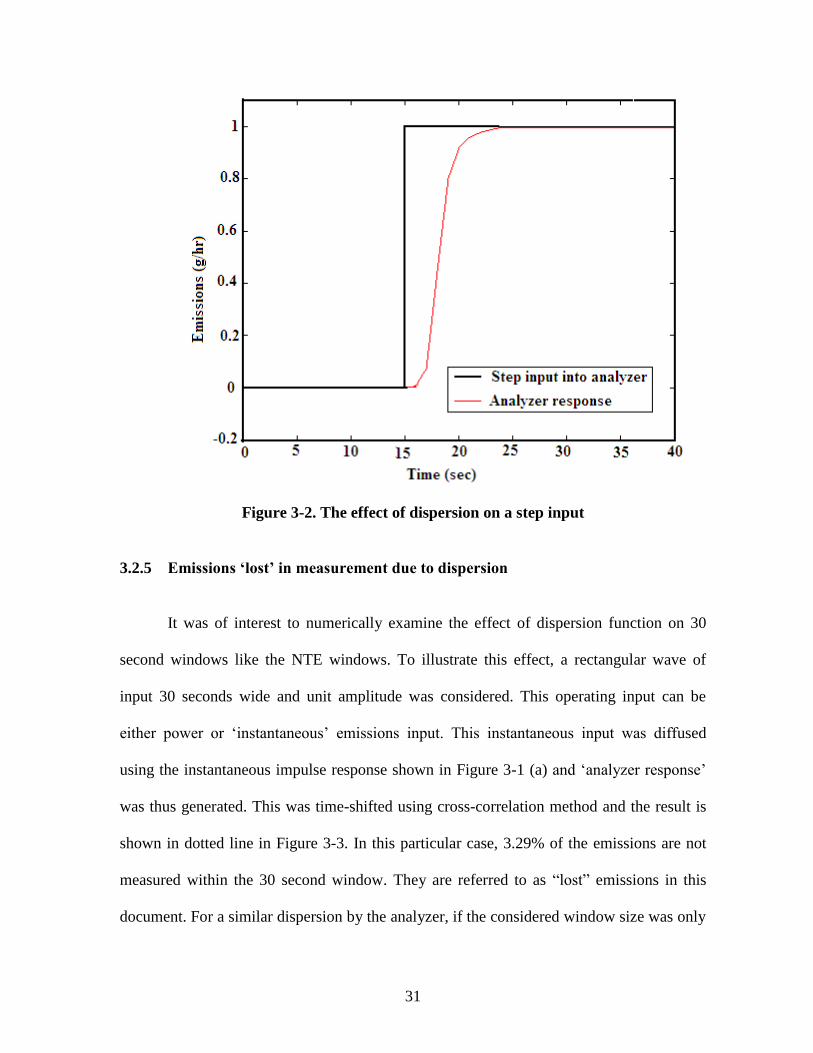
3.2.4 Understanding the effects of dispersion on a step input

The dispersion function of an analyzer is by definition, the analyzer‟s response to a

unit instantaneous impulse. Hence, the set of fractions shown as points in Figure 3-1 (a)

was in fact, the dispersion function for the Rosemount 955 NOx analyzer. To understand

the effect of such a dispersion function on instantaneous data, a hypothetical step was input

to the analyzer. The step input is dispersed using the dispersion function (the unit impulse

response) in Figure 3-1 (a). The step input and the dispersed output were shown in Figure

3-2. The response values are connected with simple straight lines in Figure 3-2. The

response takes time to reach steady state value, which is indicative of the dispersion

characteristics of the analyzer. The 10-90% response time was 2.3 seconds for this

analyzer. The 10- 90% response time specified by the manufacturer for this analyzer was in

the range of 1.5 to 2 seconds.

31

Figure 3-2. The effect of dispersion on a step input

3.2.5 Emissions ‘lost’ in measurement due to dispersion

It was of interest to numerically examine the effect of dispersion function on 30

second windows like the NTE windows. To illustrate this effect, a rectangular wave of

input 30 seconds wide and unit amplitude was considered. This operating input can be

either power or „instantaneous‟ emissions input. This instantaneous input was diffused

using the instantaneous impulse response shown in Figure 3-1 (a) and „analyzer response‟

was thus generated. This was time-shifted using cross-correlation method and the result is

shown in dotted line in Figure 3-3. In this particular case, 3.29% of the emissions are not

measured within the 30 second window. They are referred to as “lost” emissions in this

document. For a similar dispersion by the analyzer, if the considered window size was only

32

10 seconds, then 10.03% of total emissions would be lost as shown in Figure 3-4. Figure 3-

5 shows the effect of window size on lost emissions.

It should be noted that different analyzers have different response characteristics

and the responses shown in Figures 3-3, 3-4 and 3-5 are specific to the Rosemount 955

NOx analyzer with impulse response discussed in Figure 3-1 (a). However, if an analyzer

slower (or faster) than the Rosemount 955 were used, more (or less) emissions would have

been lost as shown in Figure 3-5.

Figure 3-3. The effect of dispersion on a 30-second rectangular wave

33

Figure 3-4. The effect of dispersion on a 10 second rectangular wave

34

0

2

4

6

8

10

12

14

0 10 20 30 40 50 60 70 80Window size (sec)

Per

cen

t o

f lo

st e

mis

sio

ns

Rosemount 955 A 'slower' analyzer A 'faster' analyzer

Figure 3-5. Percent of lost emissions as a function of window size

3.2.6 The ‘gain’ of emissions that corresponds to the ‘loss’ of emissions

Since the analyzer dispersion function is normalized, i.e., all the elements of the

dispersion function add up to unity, there are actually no emissions lost during the total

time of measurement. In other words, the sum total of the emissions lost in all the windows

should be gained totally in some other windows.

35

3.2.7 Amplitude reduction due to dispersion of data

When the data are dispersed by the analyzer, the maximum amplitude is under-read

and the minimum amplitude is over-read. To illustrate this effect, a sine wave is considered

and the amplitude of sine wave before and after the dispersion is measured. The frequency

of the dispersion function (the same as in Figure 3-1 (a)) was kept the same for this

analysis. When the data has a low frequency, the reduction in amplitude is lesser than for

high frequency data as shown in Figure 3-6.

0 5 10 15 20 250.95

0.96

0.97

0.98

0.99

1

Frequency of the data (hertz)

Am

pli

tud

e R

ati

o

Figure 3-6. Amplitude reduction due to dispersion of data

36

4 Experimental Equipment, Procedures and Available Data

This chapter discusses the details of the measurement equipment, the procedures

followed in the laboratories to obtain the continuous emissions data and a detailed

description of the drive cycles employed and the types of engines tested.

4.1 Operation of the engine test cell

The experimental data used for analysis in this research were obtained from

research efforts of the engineers and the technical staff who conducted engine tests at West

Virginia University Engine and Emissions Research Laboratory (WVU-EERL). A detailed

description of the test cell set up and the operation of the dynamometer and exhaust gas

sampling systems can be obtained elsewhere [69, 70]. However, a brief description of the

operation of the test cell is as follows. The engine was coupled to a dynamometer to

simulate the real world operation. The dynamometer was a DC General Electric model

DYC-243 engine dynamometer. Torque on the engine was measured by a load cell,

attached to an arm of known length, which measured force. Engine speed was recorded

with a digital encoder inside the dynamometer. The exhaust from the engine was diluted in

a full scale dilution tunnel where it was mixed with ambient air. The mass flow rate of the

diluted exhaust was measured and metered by a critical flow venturi. Sample probes were

inserted into the dilution tunnel at about 10 tunnel diameters downstream and the heated

sample lines were connected to them. The heated lines were maintained at about 235°F to

prevent any possible condensation of water vapor in the exhaust. The diluted exhaust was

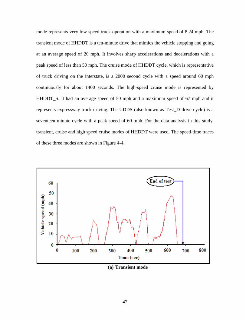
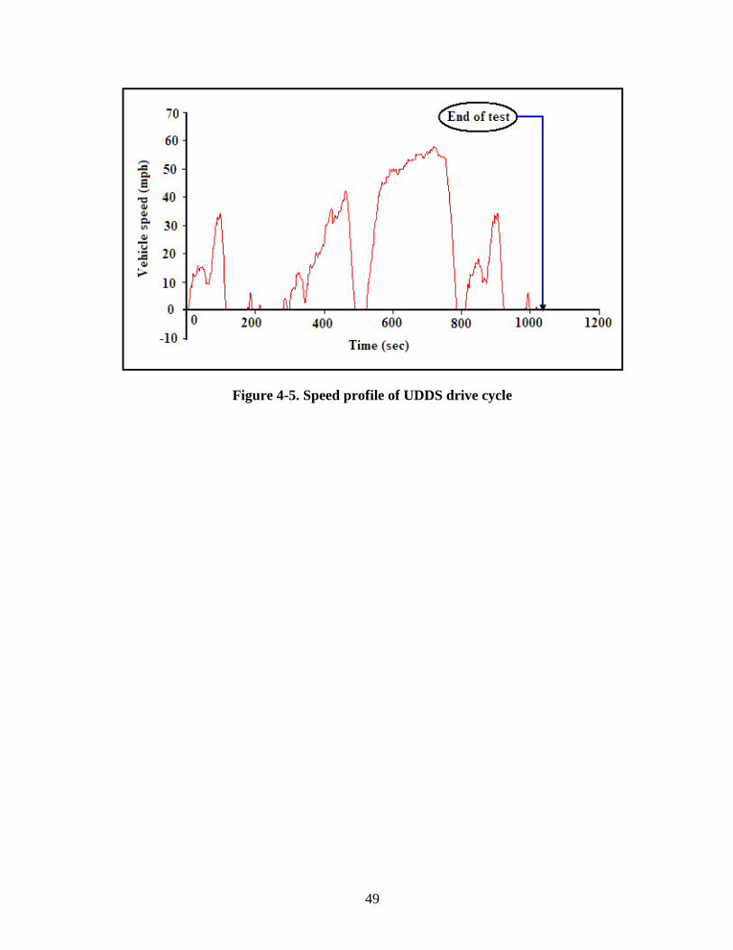
37

then carried to the analyzer sample bench shown in Figure 4-1 for analysis of exhaust

components.

4.2 Analyzers used for emissions measurement

The analyzer bench at the WVU engine test cell is shown in Figure 4-1. Further, a

brief description of the working principles for each of the analyzers is given in Table 4-1. A

more elaborate description of the working principles of all these analyzers can be found

elsewhere [71, 72].

Figure 4-1. Emissions bench at WVU-engine test cell

38

Table 4-1. Working principles of the analyzers for each of

the exhaust gas components

Component Analyzer Principle of detection 10-90 %

response time

CO HORIBA AIA

210 LE

Non-dispersive Infrared

Detector (NDIR) 2 to 5 sec

CO2 HORIBA

AIA-210

NDIR

2 to 5 sec

HC Rosemount 402 Heated Flame Ionization

Detector (HFID) 1 to 2 sec

Regular NOx Rosemount 955 Chemiluminescent Detector 1.5 to 2 sec

Fast NOx Cambustion

fNOx 400 Chemiluminescent Detector 0.012 sec

4.2.1 CO and CO2 analyzers

To analyze CO and CO2, Horiba‟s non-dispersive infra-red (NDIR) analyzers were

employed. Before the exhaust gas sample enters the analyzer, the sample is dried to avoid

moisture. There is a particular wave length of the infrared energy at which each of the

gaseous components is absorbed. The amount of energy absorbed at a wavelength

corresponding to CO (or CO2) could be measured and is directly proportional to the

concentration of CO (or CO2) in the exhaust.

39

4.2.2 HC analyzer

An internal pump was used to draw the diluted exhaust into a Rosemount Analytical

402 heated flame ionization detector (HFID) which was used to analyze hydrocarbons. The

hydrocarbons in the diluted exhaust were ionized to produce a current proportional to the

number of hydrocarbons.

4.2.3 Regular NOx analyzer

A Rosemount 955 chemiluminescent analyzer was used to measure NOx. The

analyzer worked on a phenomenon called chemiluminescence in which photons of light

were produced by a chemical or electrochemical reaction. The analyzer is capable of

measuring either NO or total NOx.

To determine NO, the sample NO is converted to NO2 by oxidation using molecular

ozone. During this reaction, about 10% of NO2 molecules get elevated to an excited state

and then when the molecules come back to non-excited state, photon emission takes place.

The emitted photons are detected and the response of the analyzer is proportional to the

total NO in the converted sample.

To determine the total NOx, a similar procedure was followed, except that the gas

stream was passed through a converter which converts all the NO2 into NO. The instrument

response in this case, is proportional to the NO present in the original sample plus the NO

produced by the dissociation of NO2.

40

4.2.4 Fast NOx analyzer

Regular NOx analyzers are most suited for an accurate estimate of the integrated

emissions collected over an entire test cycle. However, fast NOx analyzer is tailor-made for

measurement of instantaneous emissions under changing operating conditions. The

fundamental advantage of the fast NOx analyzer is that it has a rapid response (T10-90% = 12

milliseconds). This response time is the summation of the time taken by the gas to flow into

the system and the electronic delay in measurement. The fast NOx analyzer employed in the

WVU test cell was manufactured by Cambustion Ltd, Cambridge, UK [73]. The instrument

is designated as fNOx 400, and the sampling unit is shown in Figure 4-2 (a). This analyzer

is capable of measuring only NO. A comprehensive working manual [74] was provided by

Cambustion Ltd.

Figure 4-2 (a) Fast NOx sampling unit

41

The fast NOx analyzer consists of a sampling head, which was mounted close to the

dilution tunnel, as shown in Figure 4-2 (b). A sampling probe was used to connect the

sampling head to the dilution tunnel. The sampling head also consists of a constant pressure

chamber in order to stabilize the pressure fluctuations. A portion of the sample flow was

drawn into the reaction chamber of the sampling head, where it is mixed with a controlled

flow of ozone. This light was collected with the help of a fiber optic cable and measured at

the Main Control Unit (MCU) by a photo-multiplier. The MCU contained two main sub-

systems: A gas handling system that provided ozone to the sample head and an electronic

system that detected and amplified the chemiluminescence signal. The light emission was

proportional to the concentration of NO in the sample. Since the fast NOx sample was not

dried before entering the analyzer, it may have water vapor. The sampling line was heated

by a line heater controller (LHC) to avoid condensation of water vapor.

Figure 4-2 (b). Remote Sampling head of Fast NOx mounted on the dilution tunnel

42

4.3 Engine data used in the analysis

The data were obtained from the engines that were tested on Federal Transient

Procedure (FTP) at the engine test cell. The specifications of the engines are given in Table

4-2, while the cycle speed and torque of the engine are shown in Figure 4-3.

Table 4-2. Details of the engines tested on the engine dynamometer

Engine

Manufacturer

Detroit Diesel

Corporation (DDC)

Cummins

Engine Inc. Caterpillar

Engine Model Series 60 ISM 370 ESP 3406E

Model Year 2000 2004 1996

Displacement 12.7 liters 10.8 liters 14.6 liters

Power Rating 500 hp @ 2100 rpm 370 hp @ 2100 rpm 475 hp @ 2100 rpm

Torque Rating 1735 lb-ft @1450 rpm 1350 lb-ft @ 1200 rpm 1650 lb-ft @1200 rpm

Configuration Inline 6 cylinder Inline 6 cylinder Inline 6 cylinder

Bore X Stroke 5.1 in X 6.3 in 4.9 in X 5.8 in 5.4 in X 6.5 in

43

500

700

900

1100

1300

1500

1700

1900

2100

1 101 201 301 401 501 601 701 801 901 1001 1101

Time (sec)

En

gin

e sp

eed

(rp

m)

.

End of test

(a)

-700

-200

300

800

1300

1800

2300

1 82 163 244 325 406 487 568 649 730 811 892 973 1054 1135

Time (sec)

To

rqu

e (N

m)

.

End of test

(b)

Figure 4-3. Speed (a) and torque (b) profiles of DDC Series 60 engine on FTP cycle

44

4.4 Chassis dynamometer testing procedure

Some of the data analyzed in this work were obtained from the research efforts of

the engineers and the technical staff who conducted chassis dynamometer testing at the

West Virginia University Transportable Heavy-Duty Vehicle Emissions Testing

Laboratories (TRANSLAB). While a comprehensive explanation of the experimental

procedures can be found in some earlier work [75-79], a brief description of the

experimental set up is as follows. The dynamometer was a platform with flywheels, power

absorbers and rollers. The vehicle was mounted on a test bed with the drive wheels on four

rollers, two on each side. The rear wheels were allowed to rotate freely on the rollers. The

power was absorbed from the vehicle hubs by the power absorbers mounted on either side

of the chassis bed, simulating the load on the vehicle. The power absorbers simulate real-

world driving conditions by accounting for the aerodynamic and the frictional load. The

flywheels were connected to the vehicle hubs and the vehicle load was established using a

coast down procedure on the dynamometer. The torque produced by the vehicle was

translated to the sensors through shafts and gear boxes. The sum of the readings of the

sensors on either side should be equivalent to the axle torque. The vehicle was driven to

follow the speed-time trace of the desired drive cycle. The target speed was provided on the

computer screen to the driver while the test was running and the vehicle was driven to meet

that speed which simulates the drive cycle used. The emissions were measured with

exhaust gas analyzers and a data acquisition system which consists of control system

computer, driver‟s interface computer, data acquisition boards, dynamometer controllers,

sensors and calibration and testing software. The losses associated with the tire-roller

interaction have been discussed elsewhere [80].

45

4.5 Chassis data used for analysis

4.5.1 Vehicles tested on the chassis dynamometer

Some of the chassis data used in this study were obtained from the testing

conducted in the WVU Transportable Heavy-Duty Vehicle Emissions Testing Laboratory

on E55/59 CRC heavy-duty trucks [81]. The vehicles were loaded at three possible test

weights of 30,000, 56,000, and 66,000 lbs. The trucks that were tested were identified as

CRC-34, CRC-38, CRC-39 and CRC-40. Two of these trucks, CRC-34 and CRC-40, had

engines manufactured by Detroit Diesel, and two others, CRC-38 and CRC-39, had engines

manufactured by Cummins. All these engines were equipped with a cooled EGR to reduce

the emissions of NOx [82-85]. EGR is considered most effective in reducing NOx at high

loads of engine operation [86]. Chassis data were also collected from the chassis testing

conducted in on a Peterbilt Truck with a Caterpillar 3406E engine fitted to a 19-speed

Eaton Fuller transmission with 550 hp. The specifications of the trucks are presented in the

Table 4-3. Data were also collected from chassis testing conducted on a New Flyer transit

bus with 2006 Cummins ISM engine.

46

Table 4-3. Details of the vehicles tested

Vehicle

Identity

Vehicle

Model

year

Engine Engine hp &

Displacement

CRC-34 2004 DDC Series 60 500 hp & 12.7 liters

CRC-38 2004 Cummins ISX 530 hp & 15 liters

CRC-39 2004 Cummins ISX 530 hp & 15 liters

CRC-40 2004 DDC Series 60 500 hp & 14 liters

Peterbilt 2006 Cat 3406E 475 hp & 15.1 liters

New Flyer

Transit bus 2006 Cummins ISM 280 hp & 10.9 liters

4.5.2 Drive cycles used for the chassis dynamometer data

The drive cycles suitable for trucks and buses for chassis dynamometer testing have

been presented previously [87]. The chassis testing was performed on the several modes of

the Heavy Heavy-Duty Diesel Truck (HHDDT) drive schedule [Figure 4-4] and Urban

Dynamometer Driving Schedule (UDDS) [Figure 4-5]. The development and examination

of HHDDT schedule was presented in detail else where [88, 89]. The HHDDT schedule

consists of five modes (Idle, Creep, Transient, Cruise and High-speed Cruise). The creep

47

mode represents very low speed truck operation with a maximum speed of 8.24 mph. The

transient mode of HHDDT is a ten-minute drive that mimics the vehicle stopping and going

at an average speed of 20 mph. It involves sharp accelerations and decelerations with a

peak speed of less than 50 mph. The cruise mode of HHDDT cycle, which is representative

of truck driving on the interstate, is a 2000 second cycle with a speed around 60 mph

continuously for about 1400 seconds. The high-speed cruise mode is represented by

HHDDT_S. It had an average speed of 50 mph and a maximum speed of 67 mph and it

represents expressway truck driving. The UDDS (also known as Test_D drive cycle) is a

seventeen minute cycle with a peak speed of 60 mph. For the data analysis in this study,

transient, cruise and high speed cruise modes of HHDDT were used. The speed-time traces

of these three modes are shown in Figure 4-4.

(a) Transient mode

48

(b) Cruise mode

(c) High speed cruise mode

Figure 4-4. Speed profiles of different modes of HHDDT drive cycle

49

Figure 4-5. Speed profile of UDDS drive cycle

50

5 Data Analysis and Results

In this chapter, first, the „forward transform‟ was introduced and then verified by

applying the dispersion function to an operating variable, the axle power. Later, several

methods of reconstruction (back transform) were presented and validated using the real-

time emissions data.

5.1 Applying the forward transform

A „forward transform‟ is simply an application of dispersion to an instantaneous

data. In other words, if any instantaneous data is forward transformed, it generates

corresponding dispersed data. In order to reconstruct the true instantaneous emissions, the

measured emissions of the analyzer need to be back-transformed based on the dispersion

characteristics of the analyzer system employed. The dispersion characteristics were

obtained from the laboratory testing as described earlier in Chapter 3. Before attempting a

back-transformation, the dispersion characteristics were tested with a simple forward

transform. In order to achieve that, a reliable instantaneous data were required.

5.1.1 Operating variables that can simulate instantaneous data

Several studies were conducted to determine the most significant vehicle operating

parameter that can estimate the emission levels [90]. Some studies [91] concluded that

vehicle speed and acceleration could account for the emission estimation. Since

acceleration rates are very low in heavy-duty trucks, it was suggested that “instead of using

51

both acceleration and speed as independent variables, power can be used as a single

independent variable to model the NOx and CO2” [92]. Some of the emissions prediction

models involve only axle power as an operating parameter that could affect emissions.

Ramamurthy and Clark have developed models which predict emissions based on axle-

power as a single independent variable [93]. These models could predict NOx and CO2 for

one driving cycle on the basis of the model developed for another driving cycle. According

to their study, axle power as a lone parameter provided a good estimate of instantaneous

NOx. For this study, axle power was considered instantaneous and forward transform was

tested by dispersing the axle power.

5.1.2 Applying the forward transform to axle power

Before attempting a backward transform from the measured emissions which could

have several constraints on emissions data and issues such as numerical instabilities [94],

the dispersion of the emission data was simulated by dispersing the axle power [95]. The

dispersion function (discussed earlier in Chapter 2) represents the response of the analyzer

to a unit instantaneous pulse. Since the emissions measured by the analyzer are dispersed,

when they are compared against power, the power needs to be dispersed to negate the

effect of dispersion. The dispersion function of the analyzer system was used to disperse

the axle power. Even though „dispersed axle power‟ does not have any significance,

dispersing the axle power can account for the dispersion associated with the emissions data.

52

5.1.3 The effect of dispersion of axle power

Figure 5-1 shows the effects of dispersion for the data collected from CRC-34 truck

loaded at 56,000 lb and tested on the HHDDT cycle. The correlation between the time-

shifted CO2 and dispersed axle power was found to be better than the correlation between

the time-shifted CO2 and un-dispersed axle power. In both the above cases, the data were

time-aligned using the cross correlation method mentioned earlier. This was done to isolate

the effect of dispersion. Without the dispersion of axle power, the idle intercept was high

and the idle emissions had multiple values along the emissions axis. But if the power were

dispersed, most of the zero power values were eliminated leading to a smaller intercept.

y = -0.0005x2 + 0.325x + 3.9244

R2 = 0.8637

y = -0.0002x2 + 0.2268x + 10.143

R2 = 0.7927

0

10

20

30

40

50

60

70

80

0 50 100 150 200 250 300 350Axle power (kw)

Tim

e- a

lign

ed C

O 2 (

g/s

ec)

Carbon dioxide (Dispersed Power) Carbon dioxide (Undispersed Power)

Poly. (Carbon dioxide (Dispersed Power)) Poly. (Carbon dioxide (Undispersed Power))

Figure 5-1. The effect of dispersion on the correlation between emission rate and axle

power for CRC-34 loaded with 56,000 lb and tested on HHDDT_S

53

The forward transform was tested in section 5.1.2 and 5.1.3. The emissions

correlated better when the axle power (assumed instantaneous) was dispersed. Hence, if the

emissions were back-transformed, they will correlate better with axle power i.e., they will

become instantaneous.

5.1.4 Constraint on emissions data for back-transformation

Continuous data from heavy-duty testing usually stretch for about 1000 seconds and

the reconstruction was stable up to around 1000 computations. But when a 5 hertz data

were considered, the number of computation in the back transform will be 5000, thereby

causing numerical errors that made the methods unstable. The criterion for stability of each

of the methods was described in section 5.2. Hence, to ensure stability and all the data and

the dispersion functions were reduced to 1 hertz.

5.1.5 Assumptions for the analyzer system

For all the analysis in this study, the analyzer system is assumed to be time-

invariant and linear. The time-invariance of a system is illustrated in Figure 5-2 (a). For a

given input at time t1, the corresponding input is at t2. For a system to be time-invariant, the

following condition should be met. If the input is shifted by dt, then the output should

retain its earlier shape, but should shifted by dt. The linearity of the system is illustrated in

Figure 5-2 (b). Y1(t) and Y2(t) are the corresponding outputs for the inputs X1(t) and X2(t).

If the input is the summation of the two inputs X1(t) + X2(t), then the output should be the

summation of the two outputs Y1(t) + Y2(t) for the system to be linear.

54

Figure 5-2 (a) Illustration of time-invariance of the system

Time invariant system

Time invariant system

t1+dt

t2 t1

t2+ dt

55

Figure 5-2 (b) Illustration of linearity of the system

5.2 Introduction and application of back-transformation techniques

Four different back-transformation (reconstruction) techniques are presented in this

study. They are

1. Sequential Inversion Technique (SIT)

2. Differential Coefficients Method (DCM)

3. Inverse Fast Fourier Transform (IFFT)

4. Modified Deconvolution Technique (MDT)

Linear system

Linear system

Linear system

X1(t)

X2(t)

Y1(t)

Y2(t)

Y1(t)+Y2(t)

X1(t) +X2(t)

56

5.2.1 Sequential inversion technique (SIT) [96]

5.2.1.1 Theory of SIT

Let U(tj) and Y(tj) be the input and the output in the jth

second respectively. Let the

elements in the dispersion function be C1, C2, C3 and so on. The dispersion function

relates the input and output at each second as follows.

Y(t1) = C1U(t1)

Y(t2) = C1U(t2)+ C2U(t1)

Y(t3) = C1U(t3)+ C2U(t2)+ C3U(t1)

In short, the set of equations can be represented by a system as shown in Eq. 5-1.

Y(tj) = C1U(tj) + C2U(tj-1) + C3U(tj-2) + …+ CkU(tj-k+1) Eq. 5-1

where j takes values from 1 to n (where n is the number of seconds of the output data

considered) and k represents the number of elements in the dispersion function. The set of

equations can be solved in sequence starting from the first equation when j=1. Since the

computation of the input at any time interval, U(tj) from the output, Y(tj) depends on the

input at the previous time interval, U(tj-1), numerical errors will be propagated throughout

the computation. The computational error includes the loss of significant digits due to

truncation and the magnitude of the error increases with the number of data points or time

intervals.

57

5.2.1.2 The role of dispersion function on SIT

For a dispersion function {C1 C2 C3 C4}, the role played by the size of C1 was

examined keeping the other elements C2, C3 and C4 equal. (It should be noted that still C1

+C2 +C3 +C4 = 1 to achieve mass balance.) To start with, the fast NOx (from Cambustion

fNOx analyzer, introduced in Chapter 3) data were collected from the testing conducted on

1992 DDC Series 60 on 2/28/2005 at the WVU engine test cell. These data were

considered as instantaneous NOx. The data were dispersed in time using a dispersion

function to obtain the diffused data. Before considering the realistic dispersion

characteristic of an analyzer, the reconstruction of the emission signal for a simple

dispersion function such as {0.4 0.2 0.2 0.2} was examined. For this dispersion function,

the computation involved division by a large value of C1, and the input in the first time

interval was computed accurately. Consequently, the reconstruction was accurate in the

subsequent time intervals. As can be seen in Figure 5-2 (a), the reconstructed input values

(asterisks) appear to lie on the analyzer input data line. The diffused output when plotted

against the original fast NOx data was scattered as shown in Figure 5-2 (b), but the

reconstructed input agreed well (R2 of 0.999) with the fast NOx data.

58

(a)

(b)

Figure 5-3. Reconstruction using SIT (a) continuous emission (b) parity plot

The original Fast NOx data and the corresponding dispersed data were presented in Figure

5-4 (a). However, it was observed that when the value of C1 was decreased, the technique

59

failed. To find the value of C1 at which this technique begins to fail, the first element was

gradually decreased. When it was reduced to 0.137, a deviation was of the order of 1010

as

shown in Figure 5-4 (b). The deviation was noted to be oscillatory. By further reducing the

first element C1 to 0.130, the size of the deviation increased to the order of 1013

.

0 20 40 60 80 100 120 1400

200

400

600

800

1000

1200

Time (sec)

NO

x (

pp

m)

Original Fast NOx Data

Dispersed Output

(a)

60

0 20 40 60 80 100 120-8

-6

-4

-2

0

2

4

6x 10

10

Time (sec)

NO

x (

pp

m)

Reconstructed Input

(b)

Figure 5-4. SIT applied to a NOx analyzer

(a) Original data and dispersed data (b) Reconstructed data

If the first element (C1) of the diffusion function were 0.6, the magnitude of the error

(which is the difference in the amplitude of the reconstructed signal and the real signal) was

found to be of the order of 10-15

, but with the decrease of the first element, the order of the

error increased exponentially. The logarithm to the base ten of the error was computed and

was plotted against the magnitude of the first element in Figure 5-5. The order of the error

also increased with the time interval at which the error was computed. This was because

the number of computations for the reconstruction increased the error sequentially.

61

Figure 5-5. The effect C1 on order of the error in SIT

Hence, for the SIT to predict the true engine-out emissions accurately, it is

necessary that the first element of the dispersion function should be higher than the rest of

the elements. This requires that the response of the analyzer in the first time interval should

be bigger than or at least comparable to the response in the following time intervals. As this

is not the case for most dilution and analyzer systems, the examination of the cases with the

realistic dispersion function is unnecessary. Since the numerical error increases

exponentially for every computation, this method is not practical for reconstructing the

emission signal from the data measured by the current analyzer systems. Hence an effort to

reconstruct the instantaneous emissions using SIT, for the realistic diffusion function is not

warranted. In other words, since SIT failed for simple diffusion function, it will fail for a

realistic diffusion function as well.

62

5.2.2 Differential coefficients method (DCM)

Ajtay and Weilenmann have presented and discussed a mathematical approach [97]

to reconstruct the true emission signals from the measured output of the analyzer.

5.2.2.1 Definition and implementation of DCM

Following their analysis, let U(t) be the input to the analyzer and Y(t) be the

output and Y/(t) and Y

//(t) be the first and second derivatives of the output. The method

assumes that the input can be expressed as the sum of the output and some linear

combinations of the first and second derivatives of the output. The input U(t) and output

Y(t) and its derivatives are related by the following expression.

U(t) = Y(t) + a1Y/(t) + a2Y

//(t) Eq. 5-2

Eq.5-2 is subject to a constraint that the integrated input is the same as the

integrated output over the duration of observation as it is assumed that the analyzer

accounts for all of the data even though the data are delayed and diffused. This dispersion

function was considered as the output Y(t) and was differentiated numerically to obtain

Y/(t) and Y

//(t) over a period of the dispersion. These time steps for the numerical

differentiation can be one second, half a second or one tenth of a second, but a one second

time step was considered. The numerical derivatives for this study were computed using

backward differences in one second time intervals. Then the derivatives were mapped with

the unit impulse input and the time sequence was fit over the dispersion period and the

error was then computed at each second as the absolute value of [U(t) - Y(t) - a1Y/(t) -

63

a2Y//(t)]. The least squares error was computed as the sum of the squares of the computed

errors at all points and this was minimized for the best fit that generated the values of a1

and a2, the coefficients of the derivatives of the output. The values of a1 and a2 were then

used to obtain the input U of the analyzer from the output Y of any given data from the

analyzer. The inherent assumption in the method was that the analyzer was consistent in its

dispersion behavior and that its behavior will not change in the long run.

5.2.2.2 Validating DCM

5.2.2.2.1 Validating DCM in reconstructing NOx data

The fast NOx data (from the DDC Series 60) were again considered as

instantaneous NOx, representing the values of U(t) and were dispersed in time to generate

the diffused NOx, Y(t). Then the procedure described above was used to reconstruct the

NOx. The reconstructed input and the original fast NOx data were plotted on a time-wise

plot in Figure 5-6 (a). A portion of the 5-6 (a) is magnified in Figure 5-6 (b). The diffused

data were smoother and had lost some high frequency detail, but the reconstructed data

points lie close to the fast NOx curve, regaining the detail.

The correlation of the original input with the diffused output (with R2 of 0.9007)

is shown in Figure 5-6 (c). After reconstruction, the correlation (R2 of 0.976) with the

original fast NOx data improved.

64

(a)

(b)

65

(c)

Figure 5-6. NOx reconstruction using DCM

(a & b) Continuous data (c) Parity plot

5.2.2.2.2 Validating DCM in reconstructing CO2 data

One way to evaluate the high frequency detail in emissions data is to correlate

CO2 with power. For diesel engines, the CO2 corresponds closely to the fuel consumed, and

brake specific fuel consumption is fairly constant over much of the engine operating

envelope. The engine power data are not diffused in time, so that a high correlation of CO2

with power (particularly within the NTE, or at high power levels) suggests that the CO2

data are not excessively diffused.

The power was dispersed according to the dispersion function presented in Section

3.2.3 and then CO2 was time-aligned and expressed as a function of dispersed power. The

CO2 was better correlated (R2 of 0.978) with the dispersed power than with the un-

66

dispersed power (R2

of 0.890), which was expected because of the dispersion associated

with the measurement of the emissions. Then the continuous data were considered again

and the data were reconstructed using the DCM. The reconstructed data correlated better

(R2 of 0.950) with the un-dispersed axle power than the measured data (R

2 of 0.890) as can

be seen in Figure 5-7 (a). Moreover, the correlation of reconstructed (instantaneous) data

with the un-dispersed (instantaneous) power (R2 of 0.950) was almost as good as (about

97% of) the correlation of the measured data with the dispersed power (R2 of 0.978). A

section of the reconstruction is magnified in Figure 5-7 (b) and both the delay and the

dispersion of the data can be clearly observed. This suggested that the reconstruction

brought back the lost transient detail from the measured CO2 data. All the three FTP runs

from the DDC Series 60 engine showed similar results and the correlation coefficients

between the CO2 emissions and power are tabulated in Table 5-1. In all the three cases, the

reconstructed CO2 correlated better with the power than the measured CO2.

(a)

67

(b)

Figure 5-7. CO2 reconstruction using DCM (a) Parity plot (b) Continuous data

Table 5-1. R2 values for the three FTP runs examined to test the validity of the DCM

Correlating

Variables

CO2

vs

Power

CO2 vs Dispersed Power

(Forward transform)

Reconstructed CO2

vs Power

(Backward transform)

Run 1 0.890 0.978 0.950

Run 2 0.899 0.974 0.957

Run 3 0.887 0.979 0.947

68

5.2.2.3 Improvement of DCM

5.2.2.3.1 Effect of forward, central and backward differences

The DCM method suggested by Ajtay and Weilenmann [67, 97] involved the first

two differentials numerically computed using the backward differences. It was of interest

to check if the results can be varied if different methods of computing the derivatives can

be used.

A few cases were examined to understand the effect of the way in which

numerical derivatives were computed. The forward, central and backward differences were

independently used while computing the differentials. The DCM was used to reconstruct

the original data from the dispersed data and in each of the cases, the percent error was

computed as follows. If U(t) is the original input and Y(t) is dispersed output and if U‟(t)

represents the reconstructed input, then the percent error is computed according to Eq.5-3.

Percent Error = 2

2

))((

))(')((

tU

tUtU Eq. 5-3

In each of the cases, the root mean square (RMS) value of the error (error is the

difference between the reconstructed input and the original input) was computed, and the

RMS value of the original input was computed. The ratio of the RMS of the error to the

RMS of the original input was expressed as a percentage and the results when more

derivatives were used are shown in Table 5-2. The errors in all the cases were tabulated

(Table 5-2). Since the backward differences showed better results than the central and

69

forward differences, they were used for computing the derivatives for all the cases

examined in this study.

Table 5-2. Errors in DCM with different numerical methods

for computing the derivatives

Numerical Method

for computing the

derivatives

Forward

differences

Central

differences

Backward

differences

DDC-1 2.45% 1.91% 2.03%

DDC-2 2.65% 1.93% 2.04%

DDC-3 2.42% 1.96% 2.07%

CUMMINS-1 4.03% 4.38% 3.55%

CUMMINS-2 4.16% 4.32% 3.58%

CUMMINS-3 4.39% 4.25% 3.95%

5.2.2.3.2 Effect of multiple derivatives on DCM

Instead of using just two derivatives in Eq. 5-2 by DCM, multiple derivatives were

used (Eq. 5-3).

U(t) = Y(t) + a1Y/(t) + a2Y

//(t) + a3Y

3(t) + a4Y

4(t) + a5Y

5(t) + a6Y

6(t) Eq. 5-4

Several cases were examined for reconstruction using DCM with more derivatives. In each of

the cases, the percent error was computed as follows. If U(t) was the original input and Y(t)

was dispersed output and U‟(t) represented the reconstructed input, then the percent error was

again computed according to Eq.5-3 and the results were shown in Table 5-3. The marginal

70

advantage of using more derivatives was neglected and hence while applying DCM, only the

first two derivatives were considered as suggested originally in the method.

Table 5-3. Percent errors in DCM with multiple derivatives

Derivatives

Used

First two

Derivatives

‘suggested by

Ajtay et al. [67]’

First three

derivatives

Second

+ fourth

First four

derivatives

First five

derivatives

First six

derivatives

DDC-1 2.03 1.83 2.21 1.83 1.78 1.78

DDC-2 2.04 1.81 2.22 1.81 1.75 1.75

DDC-3 2.07 1.83 2.08 1.82 1.77 1.77

Cummins-1 3.55 3.48 3.36 3.29 3.29 3.28

Cummins-2 3.58 3.55 3.95 3.42 3.42 3.41

Cummins-3 3.95 3.82 4.82 3.29 3.60 3.57

5.2.2.4 Stability of DCM

The sum total of all the elements in the dispersion function is unity. For NOx and

CO2 analyzers presented in this study, the dispersion is of the order of 7 to 8 seconds.

Hence, a one hertz dispersion function will have 7 or 8 elements that sum up to unity. The

average magnitude of each element is about 0.12. For computing the values of the

coefficients, DCM involves numerical differentiation of the dispersion function. If five

hertz dispersion was considered, there are about 40 elements adding up to unity and the

average magnitude of each element falls to 0.024. In five hertz dispersion function was

employed, the numerical differentiation involves differentiating smaller numbers (than in

case of 1 hertz). It also involves five times more computations (than in case of 1 hertz) and

71

hence the coefficients could not be correctly computed. For this reason, DCM is

recommended only with 1 hertz data or when the elements of dispersion function are not

more than ten.

5.2.3 Fast Fourier Transform (FFT) and Inverse Fast Fourier Transform (IFFT)

In order to seek a better reconstruction technique than DCM, a few signal

processing techniques that are applicable to the emissions reconstruction were reviewed

[98, 99]. The application of Fast Fourier Transform and Inverse Fast Fourier Transform

was investigated. A convolution is an integral that expresses the amount of overlap of one

function as it is shifted over another function. A thorough introduction and illustration of

convolution is provided elsewhere [100].

5.2.3.1 Modeling the analyzer system

The system can be simply represented as in Figure 5-8. The input signal x(t) is

unknown. The measured data by the analyzer is the output y(t). The analyzer response to a

unit instantaneous pulse is represented as hm. Since the analyzers are assumed to be time-

invariant linear systems the response of the analyzers to an instantaneous pulse can be

modeled as the transfer function hm of the analyzer. Since the analyzers are assumed to be

invariant in time, there is one specific transfer function for any given analyzer.

72

Figure 5-8. Representation of the system in time domain

5.2.3.2 Theory of IFFT

A forward Fourier transform is used to change the representation of a function in

time domain to frequency domain. Fast Fourier Transform (FFT) converts a vector in time

domain into a vector in frequency domain. In time domain, each of the vectors is series of

discrete amplitude signals for a given discrete time. But, in the frequency domain, each of

these vectors transform to a value of one spectral component for a given discrete frequency.

The FFT for a given time-amplitude vector, X[n] for a sample size of N is given by

Equation 5-5 (a).

X[k] = ])/2exp()([ Niknnx , n in [0, N-1] Eq. 5-5 (a)

To illustrate this, a simple discrete time-amplitude signal such as [1, 2, 0, 4, 5] can

be considered and an FFT can be applied to this. The corresponding discrete frequency-

amplitude is given by the following vector.

[12.0000, -0.0729 + 5.2043i, -3.4271 - 2.0409i, -3.4271 + 2.0409i, -0.0729 - 5.2043i]

The inverse Fast Fourier Transform (IFFT) changes the representation of the

function in frequency amplitude vector space to a time-amplitude vector space. The IFFT

Analyzer (Filter)

hm

Input x(t) Output y(t)

73

for a given vector of discrete frequency-amplitude is generated by the inverse of the RHS

in Equation 5-5 (b)

x[n] = ])/2exp()([ NiknkX , k in [0, N-1] Eq. 5-5 (b)

This IFFT can be applied to the vector generated by the FFT, which brings back the

time-amplitude representation as [1.000, 2.000, 0.000, 4.000, 5.000]. The IFFT of the

Matlab generates only the real values for a series of time-amplitude vector space.

In the time domain, the convolution of x(t) and hm generates y(t). The

representation of the system in the time domain is given in Figure 5-8. The discrete

convolution between two functions over an infinite time range can be expressed as a

summation as in Eq. 5-6 (a)

t) x(n(t)hy(t) m

Eq. 5-6 (a)

A continuous representation of the convolution can be expressed in the finite range

[0, N] as shown by Eq. 5-6 (b).

(t)dth N

0τ)x(ty(t) m Eq. 5-6 (b)

The complicated convolution process in the time domain can be expressed as a

simple multiplication in the frequency domain as in Eq. 5-7.

Y(n) = X(n). Hw

Hence X(n) = Y(n)/ Hw. Eq. 5-7

74

Then the Inverse Fast Fourier Transform (IFFT) will bring the reconstructed signal

back into time domain.

5.2.3.3 Illustrating and validating IFFT

A brief illustration of the application of Fourier Transform is given in Figure 5-9.

Figure 5-9 (a) shows the sample input to the analyzer. Figure 5-9 (b) shows the convolution

of input and the analyzer dispersion function. The dispersion function used is the same as the

one experimentally determined in section 3.2.3. This dispersion function is considered as the

transfer function in the time domain. Figure 5-9 (c) shows reconstructed response using

IFFT. It can be visualized that the reconstructed signal by IFFT can be superimposed very

well on the original input signal. The ripples in the Figure 5-9 (c) could be attributed to the

numerical rounding errors in reconstruction. The amplitude of these ripples will be higher

with high frequency data and will increase exponentially with frequency of the data

eventually leading to instability of reconstruction.

5.2.3.4 Criterion for stability of IFFT

The criterion for stability of IFFT is investigated. Revisiting Equation 5-6,

Y(n) = X(n). Hw and X(n) = Y(n)/ Hw.

If a 5 hertz dispersion function is considered, the values of the Hw becomes smaller

and very high values are generated for X(n) and the reconstruction became unstable. This is a

problem with low-pass filters, usually encountered in signal processing. For the emissions

75

data in this study, when 5 hertz continuous data and 5 hertz dispersion function were

employed for reconstruction, the procedure became unstable. Hence all the data and the

dispersion function were reduced to 1 hertz for reconstruction.

0 10 20 30 40 50 60 700

2

4

6

8

10

12

Time (sec)

Orig

ina

l in

pu

t si

gn

al

x(t

)

(a) The original input signal plotted as a function of time

76

0 10 20 30 40 50 60 700

2

4

6

8

10

12

Time (sec)

Ou

tpu

t si

gn

al

y(t

) a

fter c

on

vo

luti

on

(b) Dispersed output signal

77

0 10 20 30 40 50 60 700

2

4

6

8

10

12

Time (sec)

Reco

nst

ru

cte

d s

ign

al

y(t

) a

fter I

FF

T

(c) The reconstructed signal using IFFT method

Figure 5-9. Illustration of FFT and IFFT

5.2.3.5 Comparing reconstruction ‘efficiency’ of IFFT and DCM

5.2.3.5.1 IFFT vs. DCM for reconstructing CO2

The data were collected from the chassis testing conducted in the WVU

Transportable Heavy-Duty Vehicle Emissions Testing Laboratory on a Peterbilt Truck with

a Caterpillar 3406E engine fitted to a 19-speed Eaton Fuller transmission with 550 hp. The

drive cycle employed was UDDS cycle. The engine power was generated by the Engine

Control Unit, which is based on the fuel consumption and the engine efficiency curves. The

78

results were analyzed with the collaborated efforts of the authors and Lijuan Wang. The

correlation of measured CO2 with power is shown in Figure 5-10 (a). In the entire analysis

of CO2, the background CO2 in the ambient air was subtracted from the measured value to

obtain the engine-out CO2. The reconstruction of the data was attempted using IFFT as

shown in Figure 5-10 (b) and then using DCM as shown in Figure 5-10 (c). The correlation

of the reconstructed (using IFFT) power with the measured power is shown in Figure 5-10

(d). While the reconstructed power has no realistic meaning, it gives an estimate of the

effectiveness of the reconstructing technique. In this case, the correlation in Figure 5-10 (d)

is lower than the correlation in Figure 5-10 (b) and 5-10 (c). This indicates that application

of either of the reconstruction techniques (DCM and IFFT) is better than not applying any.

Reconstruction results from the engine tests on 2004 Cummins ISM 370 tested on

the drive cycles FTP, TRANS and CRUISE were also presented in Table 5-4. In all these

cases, the engine power was measured from the engine dynamometer. In both the cases

(IFFT and DCM), the correlation of reconstructed emissions (CO2) with power was better

than the correlation of measured emissions (CO2) with power. However, it could not be

concluded that either of the methods could be more effective than the other in

reconstruction.

79

y = 0.0999x + 3.1012

R2 = 0.849

0

10

20

30

40

50

60

70

80

0 100 200 300 400 500 600

Engine power (hp)

Mea

sure

d C

O2 (

g/s

)

.

(a) Measured CO2 as a function of engine power

y = 0.1181x + 0.825

R2 = 0.9081

0

10

20

30

40

50

60

70

80

0 100 200 300 400 500 600

Engine power (hp)

Rec

on

stru

cted

CO

2 (

g/s

)

.

(b) Reconstructed CO2 (using IFFT) as a function of engine power

80

y = 0.1073x + 2.2714

R2 = 0.9006

0

20

40

60

80

0 100 200 300 400 500 600

Engine power (hp)

Rec

on

stru

cted

CO

2 (

g/s

) .

(c) Reconstructed CO2 (using DCM) as a function of engine power

y = 1.2776x - 8.7499

R2 = 0.8128

-200

0

200

400

600

800

1000

1200

0 100 200 300 400 500 600

Measured power (hp)

Rec

on

stru

cted

Po

wer

(h

p)

.

(d) Reconstructed power (using IFFT) as a function of measured power

Figure 5-10. Comparison of DCM and IFFT in reconstruction of CO2 emissions from

Peterbilt truck with Caterpillar 3406 E engine tested on TEST_D cycle

81

Table 5-4. Comparison of IFFT and DCM in reconstructing CO2

Engine type Test Cycle (R

2) Initial

(with power)

(R2) DCM

(with power)

(R2) IFFT

(with power)

1996 Caterpillar

3406E UDDS 0.849 0.9005 0.908

2004 CUMMINS

ISM370 FTP 0.775 0.7777 0.791

2004 CUMMINS

ISM370 CRUISE 0.7492 0.7500 0.7593

2004 CUMMINS

ISM370 TRANS 0.6604 0.6707 0.6909

5.2.3.5.2 IFFT vs. DCM for reconstructing NOx

Similar cases were examined and the reconstruction of NOx was attempted using

both DCM and IFFT approaches. The attempts for reconstruction are shown in Figure 5-11

and all the similar results were presented in Table 5-5. Neither method can be favored over

the other in reconstruction.

82

y = 0.0007x + 0.0187

R2 = 0.882

0.00

0.10

0.20

0.30

0.40

0.50

0.60

0.70

0 100 200 300 400 500 600

Engine power (hp)

Mea

sure

d N

Ox (

g/s

)

(a) Measured NOx as a function of engine power

y = 0.0009x - 0.0008

R2 = 0.8372

0.00

0.10

0.20

0.30

0.40

0.50

0.60

0.70

0 100 200 300 400 500 600

Engine power (hp)

Rec

on

stru

cted

N

Ox (

g/s

) .

(b) Reconstructed NOx (using IFFT) as a function of engine power

83

y = 0.0007x + 0.019

R2 = 0.8871

0.00

0.10

0.20

0.30

0.40

0.50

0.60

0.70

0 100 200 300 400 500 600

Engine power (hp)

Rec

on

stru

cted

NO

x (

g/s

) .

(c) Reconstructed NOX (using DCM) as a function of engine power

y = 1.007x + 42.805

R2 = 0.6319

0

100

200

300

400

500

600

700

800

900

0 100 200 300 400 500 600

Measured power (hp)

Rec

on

stru

cted

Po

wer

(h

p)

.

(d) Reconstructed power (using IFFT) as a function of measured power

Figure 5-11. Comparison of DCM and IFFT in reconstruction of NOx emissions from

Peterbilt truck with Caterpillar 3406E engine tested on UDDS cycle

84

Table 5-5 Comparison of DCM and IFFT in reconstructing NOx

Engine type Test Cycle (R

2) Initial

(with power)

(R2) DCM

(with power)

(R2) IFFT

(with power)

1996 Caterpillar

3406E UDDS 0.882 0.8871 0.8372

2004 CUMMINS

ISM370 FTP 0.7573 0.7617 0.7854

2004 CUMMINS

ISM370 CRUISE 0.7591 0.7686 0.8173

2004 CUMMINS

ISM370 TRANS 0.6535 0.6497 0.5620

5.2.4 Modified deconvolution technique (MDT)

5.2.4.1 Definition of blind-deconvolution

In case of SIT, as explained earlier in Chapter 5, a known analyzer dispersion

function, H was used. In case of a blind de-convolution, no information about the analyzer

dispersion function is warranted as input.

In actual signal processing terms, „blind deconvolution‟ is defined as a technique

which recovers the target object from the set of blurry images in the presence of an

unknown point spread function (PSF) [101]. A PSF simulates a filter, which is analogous to

a dispersion function in this study. While traditional deconvolution techniques require a

known PSF, a blind deconvolution technique also generates the PSF alongside the target

object. In anomaly, given the analyzer output, the blind de-convolution generates analyzer

input and the corresponding dispersion function associated with the analyzer. But this

technique totally failed when applied to reconstruction of automotive emissions.

85

Understanding the reasons warrants a clear knowledge about well-posed and ill-posed

problems, which are explained in section 5.2.4.2.

5.2.4.2 Reformulation of blind-deconvolution

A well-posed problem is the one that has a one and only one solution. For example,

a heated plate is placed in the center of the room and the distribution of temperature in the

room after a certain time needs to be found out, the solution is unique. But in case of the

converse, if the temperature distribution is known currently and the distribution at an

earlier time needs to be found out, the problem will be ill-posed. The blind-deconvolution

is an ill-posed problem When a problem is ill-posed it has infinite solutions. These infinite

number of solutions need to be narrowed down based on certain constraints imposed on the

If a problem is ill-posed, it needs to be re-formulated with additional assumptions.

Since the traditional blind-deconvolution is an ill-posed problem, „a priori‟

information is required for a solution to be unique and convergent [102]. In the context of

this research, this information could be either regarding the continuous input to the

analyzer or the dispersion characteristics of the analyzer. The a priori knowledge could also

include the fact that the instantaneous emissions are correlated well with power. The

dispersion characteristics should be in reasonable agreement with those calculated

experimentally (presented in Chapter 3). This analysis includes the a priori knowledge of

dispersion characteristics.

86

5.2.4.3 Theory and application of modified deconvolution technique (MDT)

5.2.4.3.1 Obtaining a priori information

The MDT uses some prior knowledge about the shape of the dispersion function and

from the past knowledge; the shape resembles a gamma distribution. A two parameter (k and θ)

gamma distribution G(t) can be represented by the Eq.5-8. This distribution was fitted to the

known analyzer dispersion function as shown in the Figure 5-12.

G (t) =

/1)/( t

k

et

Eq. 5-8

0

0.05

0.1

0.15

0.2

0.25

0.3

0.35

0.4

0.45

0.5

0 1 2 3 4 5 6 7 8

Time (sec)

Fra

ctio

n o

f re

spon

se p

er s

ec

Experimentally computed dispersion function Estimated Gamma distribution

Figure 5-12. Fitting a gamma distribution to the dispersion function

87

Equating the maximum values of the real H to the maximum of the gamma distribution and

differentiating the distribution with respect to time, as shown in Eq. 5-9 generates the equations

that yields the values of k and θ. These values were considered the a priori information and were

used while computing the back-transform.

0θ)(k,dt

dG Eq. 5-9

5.2.4.3.2 Computation of approximate output

The FFT was computed for both the output, Y and for transfer function H as referred to

earlier in Section 5.2.3. Then a simple division was employed in the frequency domain to

compute the input X and IFFT of that input will transfer the input into the time-domain. H, the

transfer function, which was computed experimentally, has exact gamma distribution

parameters k and θ. The actual dispersion function of the analyzer could have parameters that

are slightly different from the computed parameters by some margin, say 10%. The following

set of computations was done for the acceptable range of values of K and θ. We have X(n). Hw

= Y(n); Hence X(n) = Y(n)/ Hw and IFFT (X(n)) = X(t). Then the correlation of power with

the computed input X(t) was maximized. This generated the values of K and θ, which

generated the optimum dispersion function and corresponding reconstructed input.

5.2.4.3.3 Application of MDT for emission reconstruction

The data from the Peterbilt truck with Caterpillar 3406E engine tested on UDDS cycle

was again considered (the same was considered for reconstruction using IFFT) and the effect

88

of reconstruction using MDT is shown in Figure 5-13. In either case, MDT increased the

correlation of emissions with power. More importantly, the reconstructed input by MDT

correlated better (R2 of 0.9211) with power than the input generated by IFFT (R

2 of 0.9081)

and DCM (R2 of 0.9006).

y = 0.0999x + 3.1012

R2 = 0.849

y = 0.1081x + 2.1868

R2 = 0.9211

-10

0

10

20

30

40

50

60

70

80

0 100 200 300 400 500 600

Engine power (hp)

CO

2 (

g/s

)

(Measured)

(Reconstructed)

Figure 5-13 (a). MDT in reconstruction of CO2 emissions from Peterbilt truck with

Caterpillar 3406E engine tested on UDDS cycle

89

y = 0.0007x + 0.0187

R2 = 0.882

y = 0.0008x + 0.0153

R2 = 0.8852

-0.10

0.00

0.10

0.20

0.30

0.40

0.50

0.60

0.70

0 100 200 300 400 500 600

Engine power (hp)

NO

x (

g/s

)

(Reconstructed)

(Measured)

Figure 5-13 (b). MDT in reconstruction of NOx emissions from Peterbilt truck with

Caterpillar 3406E engine tested on UDDS cycle

5.2.5 Influence of the operating condition on emission reconstruction

It was of interest to examine the effects of speed and acceleration ranges on the

reconstruction procedure.

5.2.5.1 Processed data and drive cycles

Continuous emissions data were obtained from the chassis testing conducted on

New Flyer 2006 transit bus with a Cummins ISM 280 engine. The specifications of the

engine were presented in Table 4-3.The continuous data of speed and acceleration were

also considered. The bus was tested on UDDS and WMATA Bus drive cycles. The speed

profile of WMATA bus cycle is shown in Figure 5-14.

90

WMATA Bus Cycle

0

5

10

15

20

25

30

35

40

45

50

0 500 1000 1500 2000

Time (sec)

Veh

icle

sp

eed

(m

ph

) .

End of test

Figure 5-14. WMATA Bus Cycle

5.2.5.2.1 Division of the data into bins

For the analysis of the data, an operating condition of the vehicle is represented by

the speed and acceleration of the vehicle. The data from each cycle were divided into 63 (9

X 7) bins based on speed and acceleration ranges as shown in Table 5-6 (a). Each bin has a

specific speed range and specific acceleration range. For example, in case of UDDS, the

vehicle speed ranges from 0 to 57 mph. Hence the range of speeds for bins across the rows

will be from 0 to 7

57mph for the first column,

7

57mph to 2*

7

57mph for the second column

and so on. The acceleration range was divided similarly into 9 equal rows. The sum total of

the emissions in that bin were added up and averaged. The standard deviation of the

emissions in each bin was also computed. Analyzing the emissions in each of these bins

will associate the operating conditions with emissions data.

91

Table 5-6 (a). Measured CO2 (g/s) for different combinations of speed and

acceleration from a New Flyer 2006 Transit bus tested on UDDS drive cycle.

Average + standard deviation of measured CO2 (g/sec) for each bin

Increasing Speed in mph (Total speed range is divided into seven equal ranges)

Increasing

Acceleration

In m/s2

↓

[0 , 8.1 ) [8.1, 16.3) [16.3, 24.4) [24.4, 32.6) [32.6, 40.7) [40.7, 48.8)

[48.8, 57)

[-1.7, -1.4)

2.761

+2.618

3.210

+1.770

2.664

+ 2.363

3.605

+ 1.404

3.715

+ 1.154

4.106

+ 0.245

4.195

+ 0.007

[-1.4, -1.1)

-

5.418

+ 5.859

6.520

+ 7.751

5.025

+ 4.281

5.023

+ 2.894

4.491

+ 1.817

4.262

+ 0.205

[-1.1, -0.7)

-

15.840

+ 6.784

7.561

+ 8.826

9.531

+ 4.643

9.559

+ 3.695

6.475

+ 2.023

6.963

+ 2.218

[-0.7, -0.4)

10.334

+ 0.104

5.267

+ 6.781 -

4.221

+ 1.124

6.469

+ 3.059

5.745

+ 3.552

4.356

+ 0.837

[-0.4, -0.1)

14.145

+1.412

7.088

+7.587

12.996

+ 6.978

19.631

+ 9.801

21.233

+ 8.198

12.924

+ 7.188

-

[-0.1, 0.3)

-

-

16.742

+ 6.817

10.962

+ 4.055

12.547

+ 4.887

16.510

+ 9.223

-

[0.3, 0.6)

- - 21.890

+1.967

20.423

+ 5.099

20.836

+ 6.816

28.739

+ 0.710 -

[0.6, 0.9)

- - 20.797

+ 0.403

19.228

+5.043

18.882

+ 4.317 -

-

[0.9, 1.3)

- - - 25.365

+ 5.627

23.312

+ 5.773 - -

While the above procedure was followed in analyzing the measured data, same was

followed to analyze the reconstructed data as shown in Table 5-6 (b). MDT was employed

for reconstruction and the experimentally computed dispersion function was used (shown

92

in section 3.2.3). After the data were reconstructed, the emission values in each of the bins

changed. The ratio of the average emissions in each bin before and after reconstruction was

computed and plotted in Figure 5-15.

Table 5-6 (b). Reconstructed CO2 (g/s) for different combinations of speed and

acceleration from a New Flyer 2006 Transit bus tested on UDDS drive cycle.

Average + standard deviation of reconstructed CO2 (g/sec) for each bin

Increasing Speed in mph (Total speed range is divided into seven equal ranges)

Increasing

Acceleration

In m/s2

↓

[0 , 8.1 ) [8.1, 16.3) [16.3, 24.4) [24.4, 32.6) [32.6, 40.7) [40.7, 48.8)

[48.8, 57)

[-1.7, -1.4)

6.753

+ 0.626

6.996

+ 1.503

6.912

+1.013

6.506

+ 1.175

6.559

+ 1.064

7.020

+ 1.020

7.620

+ 0.104

[-1.4, -1.1)

7.326

+ 0.666

8.637

+ 3.150

8.151

+ 1.718

7.519

+ 1.476

8.187

+ 1.258

7.449

+ 0.112

7.449

+ 0.112

[-1.1, -0.7)

- 9.200

+ 1.960

8.024

+ 2.096

9.339

+ 2.186

9.121

+1.876

8.213

+ 1.225

8.458

+ 1.609

[-0.7, -0.4)

8.190

+ 0.934

8.193

+ 2.984 -

8.326

+ 1.234

9.257

+ 1.448

8.009

+ 2.139

8.429

+ 0.208

[-0.4, -0.1)

8.833

+ 0.650

8.704

+ 2.234

9.281

+ 2.096

11.455

+ 3.563

12.821

+ 3.134

9.910

+ 2.055 -

[-0.1, 0.3)

- - 10.734

+ 1.269

9.310

+ 1.911

9.669

+ 2.139

12.274

+ 3.104 -

[0.3, 0.6)

- - 11.882

+ 0.220

11.509

+ 2.282

11.654

+ 2.192

15.262

+ 0.104 -

[0.6, 0.9)

- - 11.573

+ 0.141

10.800

+ 0.830

10.864

+ 0.723 - -

[0.9, 1.3)

- - - 12.577

+ 0.974

12.290

+ 0.927 - -

93

5.2.5.3 Average emissions in each bin

The average emissions in each operating bin before and after reconstruction are

analyzed. The ratio of the average of the reconstructed emissions to the average of

measured emissions is calculated for every bin and is plotted in Figure 5-15. For UDDS

and for WMATA drive cycles, ratio increased with increase of speed. However, the ratio

decreased with acceleration. Also, for lower accelerations, for both the drive cycles, the

reconstructed emissions are about 50 to 150 percent higher than the corresponding

measured emissions for most of the bins.

However the ratio is sensitive to acceleration changes in both the cycles. The higher

the acceleration, the lower are the reconstructed emissions. This implies that the analyzer

system tends over-read by the input signal at higher accelerations such as starting from rest.

However, at lower accelerations (for most of the operating speeds), such as when the vehicle

is cruising at almost constant speed, the analyzer dispersion explains the overall amplitude

reduction. This implies that the signal of the analyzer is more reliable when the vehicle is at

constant speed than when accelerating.

Figure 5-16 (a) presents a bin in which the acceleration is zero. When the analyzer

measured emissions from such an operating condition, the dispersed signal appears as a

dotted black curve. When reconstructed, the signal is a rectangular wave represented by a

continuous line. In this case, the reconstruction concentrates the emissions explaining why

the reconstructed average is higher than the measured average. Figure 5-16 (b) represents a

case in which the vehicle is experiencing constant acceleration. Even in this case, the

reconstruction increased the average bin emissions.

94

-1.5 -1.2 -0.9 -0.5 -0.2 0.1 0.5 0.8 1.1

4.1

20.4

36.6

52.9

0

0.5

1

1.5

2

2.5

3

Average of

reconstructed/

Average of

measured

Average bin acceleration (m/s/s)

Average bin speed

(mph)

Figure 5-15 (a). The ratio of bin average of the reconstructed to measured CO2 for

New Flyer 2006 Transit bus tested on UDDS drive cycle

-2

-1.6

-1.2

-0.7

5

-0.3

0.1

0.5

0.9

1.3

3.15

15.75

28.35

40.95

0

0.5

1

1.5

2

2.5

3

Average of

Reconstructed/

Average of

measured

Average bin acceleration (m/s/s)

Average bin

speed (mph)

Figure 5-15 (b). The ratio of bin average of the reconstructed to measured CO2 for

New Flyer 2006 Transit bus tested on WMATA drive cycle

95

Figure 5-16 (a) Effect of reconstruction on bin with constant speed

Figure 5-16 (b) Effect of reconstruction on bin with constant acceleration

96

5.2.5.4 The standard deviation of emissions in each bin

The standard deviation of the emissions in each bin is computed as a percentage of the

average emissions in that particular bin. The values of percent standard deviations were

computed both before and after reconstruction. The ratio of the percent standard deviations of

reconstructed to the measured CO2 were plotted in Figure 5-17. Figure 5-17 (a) corresponds

to UDDS drive cycle and 5-17 (b) corresponds to WMATA Bus cycle. In both the cases, the

standard deviation was reduced for most bins because of reconstruction. The reason for this

can be explained from Figure 5-16 (a) and 5-16 (b), where the emissions bleed into the bin

from the adjacent bins because of the reconstruction. Hence there will be a drop in the

standard deviation. While there is no particular pattern evident in the ratio across bins, the

ratio tends to be higher at higher speeds. This implies that the „bleeding‟ is stabilized at

higher speeds.

-1.5 -1.2 -0.9 -0.5 -0.2 0.1 0.5 0.8 1.1

4.1

20.4

36.6

52.9

0

0.1

0.2

0.3

0.4

0.5

0.6

0.7

PSD of

reconstructed/

PSD of measured

Average bin acceleration (m/s/s)

Average bin speed

(mph)

Figure 5-17 (a). The ratio of percent standard deviation of the reconstructed to

measured CO2 for New Flyer 2006 Transit bus tested on UDDS drive cycle

97

-2

-1.6

-1.2

-0.7

5

-0.3

0.1

0.5

0.9

1.3

3.15

22.05

40.95

0

0.2

0.4

0.6

0.8

1

1.2

PSD of

reconstrusted/

PSDof measured

Average bin acceleration (m/s/s)

Average bin speed

(mph)

Figure 5-17 (b). The ratio of percent standard deviation of the reconstructed to

measured CO2 for New Flyer 2006 Transit bus tested on WMATA drive cycle

98

6 CONCLUSIONS AND RECOMENDATIONS

This chapter consists of summary of the entire research work, conclusions drawn from the

results, applications of this research and recommendations for extending the work.

6.1 Summary of the research

Emissions measured by the analyzer differ from the actual instantaneous emissions

because the actual data gets dispersed according to the dispersion characteristics specific to

the analyzer. The dispersion characteristics of analyzer were first determined

experimentally. Then these characteristics were used to generate a „forward transform‟ by

convolution of the instantaneous data with the dispersion function of the analyzer system.

Axle power was assumed to be instantaneous and a forward transform is applied to the axle

power to generate a dispersed axle power. The dispersed axle power is better correlated

with the measured emissions than the measured axle power, which indicates that the axle

power is better correlated with instantaneous data.

Four methods of reconstruction are presented in this study: Sequential Inversion

Technique (SIT), Differential Coefficients Method (DCM), Inverse Fast Fourier Transform

(IFFT) and Modified Deconvolution Technique (MDT). SIT failed in practical

applications. DCM involves least squares minimization and this accounts for small errors in

the computation of the dispersion function. Trials were made to improve the DCM by

adding more derivatives, and by trying different numerical ways to compute the

derivatives, but the improvements in either of the cases were minimal. IFFT was able to

reconstruct just as well as DCM; however the Fast Fourier Transform (FFT) of the

99

dispersion function should be high enough to ensure stability of the method. In other

words, the dispersion function should not have elements that were almost equal to zero for

the method to be stable.

When reconstruction was attempted using traditional blind deconvolution, the

results became unstable. Hence MDT uses some a priori information (in this case, the

dispersion characteristics of analyzer) for reconstruction. MDT employs fitting a gamma

distribution to the dispersion function and searches for the best possible distribution within

a prescribed range to improve the reconstruction. The a priori information stabilized the

reconstruction and the reconstructed emissions were found to be 3% more correlated (than

the measured emissions) with the axle power.

The measured continuous data of CO2 mass flow rate from the New Flyer 2006

transit bus was divided into several operating bins, each bin having a specific speed and

acceleration range. MDT was used to generate continuous reconstructed emissions from the

measured continuous data. This reconstructed data is again divided into identical bins

following a similar procedure. By comparing the two sets of bins, it was found that at low

accelerations, the average mass flow rate of the measured CO2 was lesser than that of the

reconstructed CO2. However, the reverse was found true at high accelerations. This was

because of the emissions bleeding from one bin to an other due to analyzer dispersion.

6.2 Conclusions

From the results obtained from the application of different reconstructing

techniques, some interesting conclusions can be drawn.

100

Primarily, it can be concluded that the emissions measured by the analyzer could be

represented as a convoluted product of unknown instantaneous emissions and the analyzer

dispersion function. A simple convolution of an instantaneous operating variable such as

axle power with a dispersion function generated an output which is more correlated with

the measured emissions. Hence, there is clearly more accurate continuous data than those

recorded by the analyzer.

Secondly, reconstruction of instantaneous emissions is more stable when the data

set is of lower frequencies. High frequency data made the reconstruction unstable. This is

primarily because of the computational errors rolling into the reconstruction.

Thirdly, the knowledge about the transient dynamics of the analyzer system is

critical for reconstruction. In other words, the experimental computation of the dispersion

function for the analyzer system needs to be trust-worthy and as accurate as possible. The

elements of the dispersion function can be fitted into a gamma distribution and the

parameters of the distribution can be given a range. This could help the reconstruction to be

more accurate by accounting for the experimental errors in computing the dispersion

function.

6.3 Recommended theme for heavy-duty emissions reconstruction

In reconstructing any continuous set of heavy duty emissions, the following theme

is recommended. Since IFFT is extremely uncomplicated, it is recommended initially for

any given set of heavy-duty emissions data and dispersion function. If the dispersion

function is determined experimentally and is trust-worthy, IFFT can be very accurate.

However, if the method becomes unstable, then DCM or MDT can be employed.

101

DCM and MDT are more complex and rugged methods and since they account for

the variations in the dispersion function, they are recommended in case when IFFT

becomes unstable or if the reconstructed emissions seem inaccurate.

6.4 Applications of the research work

6.4.1 Application in the field of inventory modeling

This work could help the instantaneous emissions inventory models such as

MOVES [38], which predict the emissions by relating emissions signals to vehicle

operating variables such as vehicle speed and acceleration. The reconstruction techniques

can be incorporated into the MOVES algorithm to compensate for the delay and dispersion

of the emissions data and when combined with the existing emission prediction technique

of this could be a powerful tool in instantaneous emissions modeling. This reconstruction

technique could be incorporated into several other emissions prediction models such as

COPERT [46]. The existing emissions inventory models could be refined using the

reconstruction techniques suggested in this research work.

6.4.2 Application of reconstruction for data analysts

The emissions reconstruction could be appreciated by the calibrators who measure

the emissions for testing and certification procedures. They can apply the reconstruction

technique to any of the emissions measured by a time-invariant analyzer system. In other

words, they can not only compensate for the delay of the emissions (as they are currently

doing with cross-correlation techniques for time-alignment of data with operating

102

conditions of the vehicle), but also for the associated dispersion in the analyzer. While the

analyzers have a specific response time, the calibrators can now estimate how much of

dispersion could be associated with the measured data.

6.4.3 Application in the field of engine certification by EPA

The EPA could apply this work in NTE certification. Currently, engines are

certified for a period of thirty seconds in an NTE window which is defined by operating

conditions of the vehicle. This study has shown that the some of the emissions in a window

could be „lost‟. Currently with a 30 second window, analysis has shown that up to 3 percent

of emissions can be lost. This study has also shown that when the vehicle is accelerating,

the emissions measurement analyzers distort the signal more than when the vehicle is

operating at steady speed. The reconstruction techniques, if applied by EPA for emissions

certification in a thirty second window, could eliminate distortions produced by the

measurement systems and produce a much clearer picture of how the vehicle behaves (with

regards to emissions) in the NTE window.

6.5 Recommendations for future work

Modified blind deconvolution presented in this research can be refined and

modified. For the given analyzer in this study, the gamma distribution generated a better fit

to the dispersion function than any other distributions did. However, for another research

study, Weibull, Gaussian, or any other distribution can be used based on the shape of the

dispersion function arising from the sampling system and analyzer.

103

It was understood through bin-wise reconstruction that the efficiency of

reconstruction depends on the operating condition of the engine or the vehicle. The fact that

the emissions correlate well with power can also be used as a priori information in

reconstructing emissions using MDT. Several models were developed by other researchers

(Wang) which involve emissions modeling based on the vehicle design and operating

parameters. These models can be used as a priori knowledge to improve the algorithm.

A complex algorithm can be developed based on the reconstruction techniques

described in this study. For example, if emissions for a 1000 second cycle have to be

reconstructed, and since the techniques for reconstruction carries numerical errors from one

computation to the other, a long series of computations could generate unstable results. In

such a case, the reconstruction can be stabilized by isolating the reconstruction for the first

100 seconds of the cycle and then check if the emissions are within an acceptable range,

and then proceed to the next 100 seconds and so on. However, this procedure may require

human inspection of the continuous data.

This study and the future research work on reconstruction techniques could be

applied by the engine certifiers, not only in the field of heavy-duty emissions, but also to

any situation where emissions are measured using a known analyzer system. Improving the

efficiency of reconstruction could lead to re-examination of the length of the windows that

can be used for certification procedure. Hopefully, this research work will be a foundation

for improving the accuracy of measurement required for certification and will take the

society one step further to breathing cleaner air.

104

REFERENCES

1. Health Effects Institute, Diesel Exhaust, A Critical Analysis of Emissions,

Exposure, and Health Effects (A Special Report of the Institute's Diesel Working Group),

Health Effects Institute, Cambridge, MA, 1995.

2. Watts, W. F. Jr., Assessment of Occupational Exposure to Diesel Emissions,

Diesel Exhaust: A Critical Analysis, pp. 107-123, Health Effects Institute, Cambridge, MA,

1995.

3. Graham, J. A., O'Neil, J., Claxton, L. D., Otto, D. A., Goldstein, B. D.,

Automobile Emissions: Primary Health Effects and Concerns, SAE Technical Paper

840908, 1984.

4. Kolomeychuk, R., Yeager, L., Spiegel, J., Yassi, A., Effects of Automotive

Emissions, Proceedings of Air Pollution Control Association, Vol. 5, pp. 31-33, 1984.

5. Morgan, W. K., Reger, R. B., Tucker, D. M., Health Effects of Diesel Emissions,

Annals of Occupational Hygiene, Vol. 41, n 6, pp. 643-658, 1997.

6. Duscio, D., Proietti, L., Giarrusso, S., Fantauzzo, R., Rapisarda, V., Calandra,

C., Health Effects of Diesel Exhaust, Advances in Air Pollution, Vol.13, pp. 387-399,

2003.

7. Environmental Protection Agency (EPA), Air Quality Index- A Guide to Air

Quality and Your Health (published on 8/31/03), Information Retrieved from the

Website:www.epa.gov on 20th May, 2007.

8. California Air Resources Board (CARB), Almanac Emission Projection Data,

Information Retrieved from the Website:www.arb.ca.gov on April 10, 2007.

105

9. Kirchstetter, W. T., Harley, A. R., Kreisberg, N. M., Stolzenburg, M. R.,

Hering, S. V., On-Road Measurement of Fine Particle and Nitrogen Oxide Emissions from

Light- and Heavy-Duty Vehicles, Atmos. Environ.1, Vol. 33, pp. 2955-2968, 1999.

10. The Environmental Literacy Council, Clean Air Act, Information Retrieved from

the Website:www.enviroliteracy.org/article.php/6.html, the Environmental Literacy

Council, 2002.

11. Thompson, G., Gautam, M., Clark, N. N., Lyons, D., Inference of Torque and

Power from Heavy-Duty Diesel Engines for On-Road Emissions Monitoring, SAE

Technical Paper 2002-01-0614, 2002.

12. Code of Federal Regulations, Title 40, Part 86, Subpart N, Emission Regulations

for New Otto-Cycle and Diesel Heavy-Duty Engines, Gaseous and Particulate Exhaust

Test Procedures, 2004.

13. Dieselnet, Emission Test Cycles: Heavy-Duty FTP Transient Cycle, Information

Retrieved from the Website:www.dieselnet.com, on 25th

June, 2006.

www.dieselnet.com/standards/cycles/ftp_trans.html

14. Dieselnet, Emission Standards: USA: Heavy-Duty Truck and Bus Engines, Information

Retrieved from the Website:www.dieselnet.com, on March 17, 2006.

www.dieselnet.com/standards/us/hd.html.

15. The Environmental Literacy Council, Clean Air Act, Information Retrieved from

the Website:www.enviroliteracy.org/article.php/6.html, on March 12, 2002.

16. Dieselnet, Diesel Emissions Online, Information Retrieved from the Website

www.dieselnet.com on Jan 17, 2005.

106

17. Dieselnet, Series 60-Still the Fuel Economy Leader, Product Brochure, Detroit

Diesel Corporation, 2005, Information Retrieved from the Website:www.dieselnet.com

on Dec 6, 2006, www.detroitdiesel.com/public/brochures/6sa303.pdf.

18. Yanowitz, J., Alleman, T. L., Ryan, L. B., McCormick, R. L., Graboski, M. S.,

Chassis Dynamometer Study of Emissions from 21 In-Use Heavy-Duty Diesel Vehicles,

Environmental Science and Technology, Vol. 33, pp. 209-216, 2000.

19. Osenga, M., Diesel Industry Confronts the Emission Settlement EPA Enforcement

of the Clean Air Act Affects Entire Diesel Engine Industry, Diesel Progress, North

American Edition, (Published on 12/1/98), 1998.

20. Federal Register, Notice of Filing a Consent Decree Under the Clean Air Act,

Office of the Federal Register, National Archives and Records Administration,

Washington, DC, Vol. 33, n 212, Nov 3, 1998.

21. Dieselnet, Applicability and Test Cycles, United States Heavy-Duty Truck and Bus

Engines, Information Retrieved from www.dieselnet.com on Aug 31, 2005.

22. Dieselnet, NTE Test Procedure and NTE Limits, Information Retrieved from the

Website:www.dieselnet.com on Aug 31, 2005.

23. Krishnamurthy, M., Characterization of In-Use Emissions from On-Highway

Heavy- Duty Diesel Engines. Masters Thesis, Department of Mechanical and Aerospace

Engineering, West Virginia University, 2003.

24. USEPA Office of Transportation and Air Quality, In Use Testing Program for

Heavy-Duty Diesel Engines and Vehicles, Technical Support Document, Document EPA

420-R-05-006, 2005.

107

25. Working Group on Off-Cycle Emissions, EPA Answers to Questions from March

22nd 2004 NTE Presentation. Information Retrieved from the Website:

http://www.oica.net on Jan 15, 2006.

26. DG Entr (Enterprise), In-Use Conformity Testing of Emissions Control Devices,

Study on Emission Control Technology for Heavy-Duty Vehicles, Study Prepared for the

European Commission, May 2002.

27. USEPA, Control of Emissions of Air Pollution from 2004 and Later Model Year

Heavy-Duty Highway Engines and Vehicles, Revision of Light-Duty Truck Definition, 40

CFR Parts 85 and 86, 1999.

28. Iddo, W., NTE Control Area Evaluation With Respect to the Real-World Engine

Operation Envelope, Prepared for the 13th Meeting of the Working Group on Off-Cycle

Emission, (Presented 5-7 April 2006), 2006.

29. USEPA, Test Plan to Determine PEMS Measurement Allowances for the Gaseous

Emissions Regulated Under the Manufacturer-run-Heavy-Duty Diesel Engine In-Use

Testing, DOCKET OAR-2004-0072-0069, (May 20, 2005) Program, 2005.

http:/www.epa.gov/otaq/highway-diesel/regs/testplan.pdf.

30. Butler, J. W., Kornisk, T. J., Reading, A. R., Kotenko, T. L., Generating

Dynamometer Quality Data On-board Vehicles for Real-World Emission Measurements,

Proceedings of the Ninth CRC On-Road Vehicle Workshop, April19-21, San Diego, CA,

1999.

31. Kihara, N., Tsukamoto, T., Matsumoto, K., Ishida, K., Kon, M., Murase, T.,

Real-time On-Board Measurement of Mass Emission of NOx, Fuel Consumption, Road

108

Load, and Engine Output for Diesel Vehicles, SAE Technical Paper No. 2000-01-1141,

2000.

32. Jetter, J., Maeshiro, S., Hatcho, S., Klebba, R., Development of an On-Board

Analyzer for Use on Advanced Low Emission Vehicles, SAE Technical Paper No. 2000-01-

1140, 2000.

33. Mackay, G. I., Nadler, S. D., Karecki, D. R., Schiff, H. I., Butler, J. W.,

Gierczak, C. A., Jesion, G., Dynamometer Inter-comparison of Automobile Exhaust Gas

CO/CO2 Ratios and Temperature Between On-Board Measurements and a Remote Sensing

Near Infrared Diode Laser System, Phase 1b Report to the Coordinating Research Council

and National Renewable Energy Laboratory, 1994.

34. Gautam, M., Clark, N. N., Lyons, D. W., Long, Jr., T. R., Howell, A. D., Loth,

J. L., Palmer, G. M., Bata, R. M., Design Overview of a Heavy Duty Mobile Vehicle

Emissions Testing Laboratory, ASME DE-VOL. 40, Advanced Auto. Tech., pp.199-207,

WAM, Atlanta, 1991.

35. Riddle, W., Design and Evaluation of the Emissions Measurement Components for

a Heavy-Duty Diesel Powered Vehicle Mobile Emissions Measurement System (MEMS),

Masters Thesis, Department of Mechanical and Aerospace Engineering, West Virginia

University, 2001.

36. Shade, B., A Performance Evaluation of the MEMS: An On-Road Emissions

Measurement System Study, Masters Thesis, Department of Mechanical and Aerospace

Engineering, West Virginia University, 2000.

37. Gautam, M., Clark, N. N., Thompson, G. J., Carder, D. K., Lyons, D. W.,

Development of In-use Testing Procedures for Heavy-Duty Diesel-Powered Vehicle

109

Emissions, Department of Mechanical and Aerospace Engineering, West Virginia

University, Morgantown, WV, 2000.

38. Koupal, J., Draft Design and Implementation Plan for EPA's Multi-Scale Motor

Vehicle and Equipment Emission System (MOVES), U.S. EPA Technical Report #420-P-

02-006, October 2002.

39. USEPA, MOVES 2004: Energy and Emission Inputs, Office of Transportation and

Air Quality, USEPA Draft Report, EPA 420-P-05-003, March 2005.

40. Weinblatt, H., Dulla, R. G., Clark, N. N., A Vehicle Activity Based Procedure for

Estimating Emissions of Heavy-Duty Vehicles, Journal of Transportation Research, TRR

1842, pp. 64-72, 2003.

41. Air Resources Board, State of California, Mobile Source Emission Inventory

Program- On Road Motor Vehicle Emission Inventory (MVEI) Models, Information

Retrieved from the world wide web, http://www .arb.ca.gov on Jan 6, 2006.

42. Brzezinski, D. J., Newell, T. P., A Revised Model for Estimation of Highway

Vehicle Emissions: Mobile6, EPA Report No.EPA-420-S-99-001, 1999.

43. Coordinating Research Council, Report CRC-APRAC-91, Proceedings of the

CRC-APRAC On-Road Vehicle Emissions Work-Shop, Los Angeles, CA, 1991.

44. Coordinating Research Council, Report CRC-APRAC-94, Proceedings of the

Fourth CRC-APRAC-94 On-Road Vehicle Emissions Work-Shop, San Diego, CA, 1994.

45. Fujita, E., Comparison of Emission Estimates and Ambient Concentrations of CO,

NOMHC and NOx in California’s South Coast Air Basin, International Specialty

Conference on Emission Inventory Issues in the 1990s, Durham, North Carolina, 1991.

110

46. Ntziachristos, L., Samaras, Z., Eggleston, S., Gorissen, N., Hassel, D.,

Hickman, A. J., Joumard, R., Rijkeboer, R., Zierock, K. H., COPERT Computer

Program to Calculate Emissions from Road Transport-Methodology and Emission Factors,

Technical Report 49, European Environment Agency, 2000.

47. Barth, M., An, F., Norbeck, J., Ross, M., Modal Emissions Modeling: A Physical

Approach, Transporation Research Record 1520, pp. 81-88, 1996.

48. Barth, M. J., The Development of a Comprehensive Modal Emission Model,

Proceedings of the Seventh CRC On-Road Vehicle Emissions Workshop, Coordinating

Research Council, Atlanta, GA, pp. 6.53- 6.71, 1997.

49. Washington, S., Wolf, J., Guensler, R., A Binary Recursive Partitioning Method

for Modeling Hot-Stabilized Emissions from Motor Vehicles, 76th Annual Meeting,

Transportation Research Board, Washington, DC, 1997.

50. Strum, J., Almbauer, R., Sudy, C., Pucher, K., Application of Computational

Methods for the Determination of Traffic Emissions, Journal of the Air & Waste

Management Association, Vol. 47, pp. 1204-1210, 1997.

51. Traver, M. L., Atkinson, R. J., Atkinson, C. M., Neural Network-Based Diesel

Engine Emissions Prediction Using In-Cylinder Combustion Pressure, SAE Technical

Paper 1999-01-1532, Warrendale, PA, 1999.

52. Jost, P., Hassel, D., Sonnborn, K., Weber, F., Emissions and Fuel Consumption

Modeling Based on Continuous Measurements, Report of the Institute of Combustion

Engines and Thermodynamics, TU-GRAZ, Austria, Vol. 64, 1992.

111

53. Andrei, P., Real World Heavy-Duty Emissions Modeling, Masters Thesis,

Department of Mechanical and Aerospace Engineering, West Virginia University, 2001.

54. Jost, P., Joumard, R., Hickman, J., Influence of Instantaneous Speed and

Acceleration on Hot Passenger Car Emissions and Fuel Consumption, SAE Technical

Paper 950928, 1995.

55. Weilenmann, M., Bach, C., Rudy, C., Aspects of Instantaneous Emissions

Measurement, International Journal of Vehicle Design, Vol. 27, pp. 94-104, 2001.

56. Messer, J. T., Clark, N. N., Lyons, D. W., Measurement Delays and Modal

Analysis for a Heavy-Duty Transportable Emissions Testing Laboratory, SAE Technical

Paper 950218, 1995.

57. Messer, J. T., Measurement Delays and Modal Analysis for Two Heavy-Duty

Transportable Emissions Testing Laboratories and a Stationary Engine Emission Testing

Laboratory, Masters Thesis, Department of Mechanical and Aerospace Engineering, West

Virginia University, 1995.

58. Hawley, J. G., Brace, C. J., Cox, A., Ketcher, D., Stark, R., Influence of Time-

Alignment on the Calculation of Mass Emissions on a Chassis Dynamometer, SAE

Technical Paper 2003-01-0395, 2003.

59. Ramamurthy, R., Heavy-Duty Emissions Inventory and Prediction, Masters

Thesis, Department of Mechanical and Aerospace Engineering, West Virginia University,

Morgantown, West Virginia, 1999.

112

60. Clark, N. N., Jarrett, R. P., Atkinson, C. M., Field Measurements of Particulate

Matter Emission and Exhaust Opacity from Heavy-Duty Vehicles, Journal of Air and Waste

Management Association, Vol. 49, pp. 76-84, 1999.

61. Hawley, J. G., Bannister, C. D., Brace, C. J., Cox, A., Ketcher, D., Stark, R.,

Further Investigations on Time-Alignment, SAE Technical Paper 2004-01-1441, 2004.

62. Levenspiel, O, Chemical Reaction Engineering, Second Edition, John Wiley &

Sons, Singapore, 1972.

63. Liang, T. F., Yong, K. A, Axial Dispersion of Solids in Rotary Solid Flow Systems,

Journal of Applied Scientific Research, Vol.10, pp. 465- 470, 2004.

64. Trinidad, P., Ponce, C. A., Walsh, F. C., the Application of Flow Dispersion

Models to the FM01-LC Laboratory Filter-Press Reactor, Electrochimica Acta, Vol. 52, n

2, pp. 604-613, 2006.

65. Ramamurthy, R., Clark, N. N., Lyons, D. W., Atkinson, C. M., Models for

Predicting Transient Heavy-Duty Vehicle Emissions, SAE Technical Paper 982652,

1998.

66. Ganesan, B., Clark, N. N., Relationship between Instantaneous and Measured

Emissions in Heavy-Duty Applications, SAE Technical Paper 2001-01-3536, 2001.

67. Weilenmann, M., Soltic, P., Ajtay, D., Describing and compensating gas

transport dynamics for accurate instantaneous emission measurements, Atmos. Environ

Vol. 37, pp. 5137-5145, 2003.

68. Pilley, A. D., The Transient Response Characteristics of Emissions Analyzers,

Ricardo International Publication DP 87/0064.

113

69. George, S., Characterization of In-Use Emissions from Marine Engines, Masters

Thesis, Department of Mechanical and Aerospace Engineering, West Virginia University,

2004.

70. Bane, B. R., A Comparison of Steady State and Transient Emissions from Heavy-

Duty Diesel Engines, Masters Thesis, Department of Mechanical and Aerospace

Engineering, West Virginia University, 2002.

71. Aravelli, A., Real Time Measurement of Oxides of Nitrogen from Heavy-Duty

Diesel Engines, Masters Thesis, Department of Mechanical and Aerospace Engineering,

West Virginia University, 2003.

72. Nayak, G. A., Development of a Test Method to Measure In-Use Emissions from

Stationary and Portable Diesel Sources, Masters Thesis, Department of Mechanical and

Aerospace Engineering, West Virginia University, 2004.

73. Cambustion, Fast Gas Analyzers, Information retrieved from the website

www.cambustion.com on June 29, 2006.

74. Cambustion Limited, fNOx 400, Users Manual.

75. Clark, N. N., Gautam, M., Bata, R. M., Loth, J. L., Palmer, G. M., Wang, W.

G., Lyons, D. W., Design and Operation of a New Transportable Emissions Laboratory

for Emissions Testing of Heavy-Duty Trucks and Buses, Heavy Vehicle Systems, Special

Series, International Journal of Vehicle Design, Vol. 21, n 6, pp. 285-299, 1995.

76. Clark, N. N., Lyons, D. W., Gautam, M., Bata, R. M., Wang, W. G., Norton, P.,

Chandler, K., Natural Gas and Diesel Transit Bus Emissions Review and Recent Data,

SAE Technical Paper 973203, 1997.

114

77. Clark, N. N., Gautam, M., Wayne, W. S., Lyons, D. W, Thompson, G., Heavy-

Duty Vehicle Chassis Dynamometer Testing for Emissions Inventory, CRC Report No. E

55/59, Coordinating Research Council, Inc. Alpharetta, GA, 2007.

78. Ferguson, D. H. ,Gautam, M., Wang, W. G., Clark, N. N., Lyons, D. W., Bata,

R. M., Palmer, G. M., Katragadda, S., Exhaust Emissions from In-Use Heavy-Duty

Vehicles Tested on a Transportable Transient Chassis Dynamometer, SAE Technical Paper

922436,1992.

79. Gautam, M., Ferguson, D. H. , Wang, W. G., Bata, R. M., Clark, N. N., Lyons,

D. W., Palmer, G. M., Katragadda, S., In-Use Emission and Performance Monitoring of

Heavy-Duty Vehicles Using a Transportable Transient Chassis Test Facility, SAE

Technical Paper 921751, 1992.

80. Salem, M. I., Mucino, V. H., Gautam, M., Speed Dependent Rolling Resistance

Evaluation of a Twin Roller Chassis Dynamometer for Heavy-Duty Vehicles, International

Journal of Computer Applications in Technology, Vol.12, pp. 349-357, 1999.

81. Clark, N. N., Gautam, M., Wayne, W. S., Lyons, D. W., Thompson, G.,

California Heavy Heavy-Duty Diesel Truck Emissions Characterization for Project E-

55/59 Phase 1.5, CRC E-55/59, Phase 1.5 Final Report, 2004.

82. Jacobs, T., Assanis, D., Filipi, Z., The Impact of Exhaust Gas Recirculation on the

Performance and Emissions of a Heavy-Duty Diesel Engine, SAE Technical Paper 2003-

01-1068, 2003.

83. Baert, R. S. G., Beckman, D. E.,Veen, A., Efficient EGR Technology for Future

Heavy-Duty Diesel Engine Emission Targets, SAE Technical Paper 1999-01-0837, 1999.

115

84. Kohketsu, S., Exhaust Gas Recirculation in Turbocharged Diesel Engines,

Proceedings of JASE Convention, 9638266, 1996.

85. Hiereth, U., Gaertner, M., Loehle, C., Pfender, H., Investigation of cooling and

recirculating exhaust gases in heavy-duty truck engines. Development of an exhaust gas

cooler, Proceedings of 18th International Vienna Motor Symposium Series, Vol. 306, pp.

321–340, 1997.

86. Yamada, T., Ikeya, N., and Kondoh, N., New EGR system for heavy duty diesel

engines, SAE Technical Paper 980775, 1998.

87. McKain, D. L., Clark, N. N., Daniel, T. I., Hoppie, J. A., Chassis Test Cycle

Development for Engine Test Compliance on Heavy-Duty Vehicles, SAE Technical Paper

980407, 1998.

88. Gautam, M., Clark, N. N., Riddle, W., Nine, R., Wayne, W. S., Maldonado, H.,

Agrawal, A., Carlock, M., Development and Initial Use of Heavy-Duty Diesel Truck Test

Schedule for Emissions Characterization, SAE Technical Paper 2002-01-1753, 2002.

89. Clark, N. N., Gautam, M., Wayne, W. S., Riddle, W., Nine, R. D., Lyons, D.

W., Xu, S., Examination of Heavy Heavy-Duty Diesel Truck Chassis Dynamometer

Schedule, SAE Technical Paper 2004-01-2904, 2004.

90. William, M. D., Thayer, G., Barth. M. J., Smith, L. L., The TRANSIMS

Approach to Emission Estimations, Report No. LA-UR-99-471, Los Alamos National

Laboratory, 1999.

116

91. Jost, P., Jourmard, R., Hickman, J., Influence of Instantaneous Speed and

Acceleration on Hot Passenger Car Emissions and Fuel Consumption, SAE Technical

Paper 950928, 1995.

92. Samuel, S., Morrey, D., Fowkes, M., Taylor, D. H. C., Austin, L., Felstead, T.,

Latham, S., The Most Significant Vehicle Operating Parameter for Real-World Emissions

Levels, SAE Technical Paper 2004-01-0636, 2004.

93. Ramamurthy, R., Clark, N. N., Lyons, D. W., Atkinson, C. M., Models for

Predicting Transient Heavy-Duty Vehicle Emissions, SAE Technical Paper 982652, 1998.

94. Madireddy, R. M., Clark, N. N., Sequential Inversion Technique and Differential

Coefficients Approach for Accurate Instantaneous Measurement, International Journal of

Engine Research, Vol. 7, pp. 437-446, 2006.

95. Ramamurthy, R., Clark, N. N., Atmospheric Emissions Inventory Data for Heavy-

Duty Vehicles, Environmental Science and Technology, Vol. 33, pp. 55-62, 1999.

96. Clark, N. N., Madireddy, M. R., Gautam, M., Wayne, S. W., Thompson, G.,

Lyons, D. W., Atmospheric Emissions Inventory Data for 2003 and Later Model-Year

Heavy-Duty Vehicles.

97. Ajtay, D., Weilenmann, M., Compensation of the exhaust gas transport dynamics

for accurate instantaneous emission measurements, Environmental Science and

Technology, Vol.38, pp. 5141-5148, 2004.

98. Beaumont, A. D., Noble, A. D., Pilley, A. D., Signal reconstruction techniques for

improved measurement of transient emissions, SAE Paper 9002333.

117

99. Daboczi, T., Kollar, I., Multi-parameter optimization of inverse filter algorithms,

IEEE Transactions on Instrumentation and Measurement. Vol. 45, pp. 417-422, 1996.

100. Smith, W. S., The scientist and engineer’s guide to digital signal processing,

Retrieved from the Website: http://www.dspguide.com/ch6.htm on Jan 14, 2008.

101. Signal reconstruction theory and its applications, Tsinghua University Press, pp.

135-138, 1991.

102. Jiang, M., Wang, G., Development of blind image deconvolution and its

applications, Journal of X-Ray Science and Technology, Vol.11, pp. 13–19, 2003.