Page 1
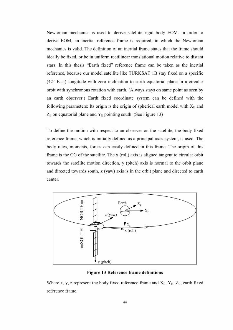
3-AXIS ATTITUDE CONTROL OF A GEOSTATIONARY SATELLITE
A THESIS SUBMITTED TO THE GRADUATE SCHOOL OF NATURAL AND APPLIED SCIENCES
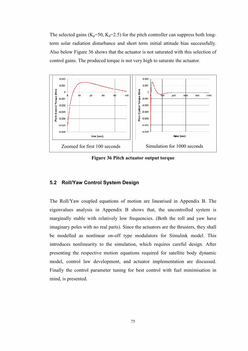
OF THE MIDDLE EAST TECHNICAL UNIVERSITY
BY
HAKKI ÖZGÜR DERMAN
IN PARTIAL FULFILMENT OF THE REQUIREMENTS FOR THE DEGREE OF
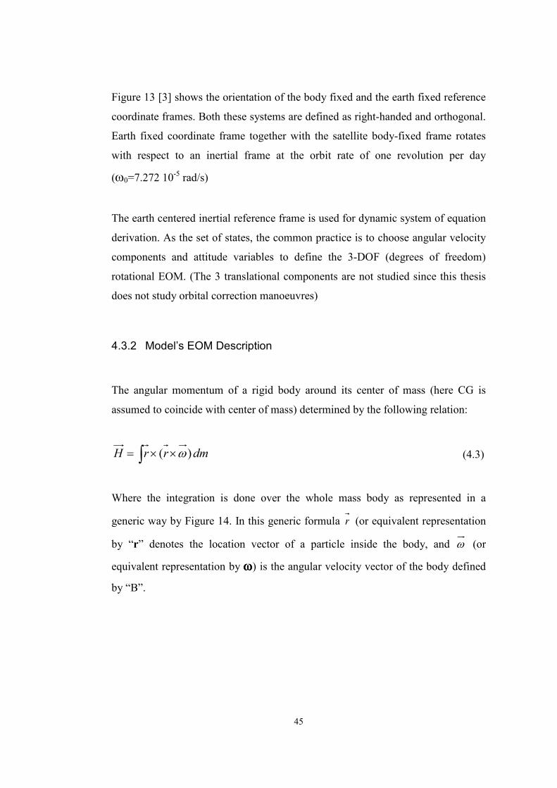
MASTER OF SCIENCE IN
THE DEPARTMENT OF AERONAUTICAL ENGINEERING
DECEMBER 1999
Page 2
ii
Approval of the Graduate School of Natural and Applied Sciences
Prof. Dr. Tayfur Öztürk Director I certify that this thesis satisfies all the requirements as thesis for the degree of Master of Science.
Prof. Dr. Nafiz Alemdaroğlu Head of Department
This is to certify that we have read this thesis and that in our opinion it is fully adequate, in scope and quality, as a thesis for the degree of Master of Science.
Prof. Dr. Yurdanur Tulunay Assoc. Prof. Dr. Ozan Tekinalp Co-Supervisor Supervisor Examining Committee Members
Prof. Dr. M. Cevdet Çelenligil
Prof. Dr. Ünver Kaynak
Assoc. Prof. Dr. Yusuf Özyörük
Assoc. Prof. Dr. Mehmet Ş. Kavsaoğlu
Assoc. Prof. Dr. Ozan Tekinalp
Page 3
iii
ABSTRACT
3-AXIS ATTITUDE CONTROL OF A GEOSTATIONARY SATELLITE
Derman, Hakkı Özgür
M.S., Department of Aeronautical Engineering
Supervisor: Assoc Prof. Dr. Ozan Tekinalp
December 1999, 134 pages
In this thesis application of an attitude control system minimising fuel expenditure
of a geostationary satellite is studied. The satellite parameters are similar to the
actual TÜRKSAT 1B satellite platform. TÜRKSAT 1B Attitude Determination
and Control Subsystem is described in detail. Using MATLAB-Simulink
computing, modelling and simulation environment, the satellite attitude, under
various external and internal disturbances and sensor noise is simulated. A new
automatic control system is designed. A PD controller regulates the pitch attitude
with strapdown momentum wheels. For yaw/roll attitude regulation, an integral
plus full state-feedback controller attitude is designed, and tested various pole
locations. Pulse width modulated thruster activation period is also tuned for fuel
expenditure minimisation through an extensive parametric search.
Key Words: Attitude Control, Geostationary Satellite, TÜRKSAT 1B, Pulse Width
Modulation, Pole Placement Design, State Variable Feedback, Attitude
Regulation, Satellite Attitude Simulations.
Page 4
iv
ÖZET
YER EŞZAMANLI BĐR UYDUNUN 3 EKSENDE DENETĐMĐ:
Derman, Hakkı Özgür
Yüksek Lisans, Havacılık Mühendisliği Bölümü
Tez Yöneticisi: Doç. Dr. Ozan Tekinalp
Aralık 1999, 134 Sayfa
Bu tezde yer eşzamanlı bir uydunun davranış hareketine yakıt sarfiyatını en aza
indiren denetim sisteminin tasarlanması incelenmiştir. Kullanılan uydu modelinin
özellikleri gerçek TÜRKSAT 1B uydusununkilere benzemektedir. TÜRKSAT 1B
davranış hareketi belirleme ve denetim altsistemi detaylıca tanıtılmıştır.
MATLAB–Simulink yazılımı kullanılarak uydunun çeşitli iç ve dış bozucu
kuvvetler ve algılayıcı gürültüsü altında davranışı için benzetim çalışması
yapılmıştır. Yeni bir denetim yasası tasarlanmıştır. Bir PD denetimcisi yunuslama
davranışını momentum tekeri ile ayarlar. Sapma/ yuvarlanma açısal denetimi için
bir tüm hal değişkenleri geribeslemesi ile bir integral denetimcisi tasarlanıp
değişik özdeğer atama yöntemi ile denenmiştir. Darbe genlik modulasyonu
kullanan tepki motorunun faaliyet devresi, yakıt sarfının en aza indirilmesi için
kapsamlı parametrik bir tarama yapılarak belirlenmiştir.
Anahtar Kelimeler: Davranış Denetimi, Yereşzamanlı Uydu, TÜRKSAT 1B,
Darbe Genlik Modulasyonu, Özdeğer Atama Tasarımı, Durum Değişkenleri
Geribeslemesi, Davranış Düzenlemesi, Uydu Davranış Benzetimi.
Page 5
v
TABLE OF CONTENTS
ABSTRACT ................................................................................................................................... III
ÖZET.............................................................................................................................................. IV
TABLE OF CONTENTS................................................................................................................V
CHAPTERS .......................................................................................................................................
I. INTRODUCTION ........................................................................................................................1
1.1 INTRODUCTION TO “ATTITUDE CONTROL OF A SATELLITE PLATFORM RESEMBLING TO
TÜRKSAT 1B” .............................................................................................................................1
II. LITERATURE SURVEY ...........................................................................................................5
2.1 SURVEY SUMMARY...............................................................................................................5
III. DESCRIPTION OF TÜRKSAT 1B SATELLITE SYSTEM WITH A
CONCENTRATION ON ATTITUDE CONTROL SUBSYSTEM ...........................................11
3.1 TÜRKSAT 1-B ON ORBIT .................................................................................................11
3.2 GENERAL DESCRIPTION OF TÜRKSAT 1B SUBSYSTEMS ...................................................13
3.3 ATTITUDE DETERMINATION AND CONTROL SUBSYSTEM (ADCS) .....................................13
3.3.1 Overall Electrical Configuration..............................................................................14
3.3.2 TÜRKSAT 1B Attitude Sensor Configuration...........................................................15
3.3.3 Attitude Determination and Control Electronics......................................................19
3.3.4 TÜRKSAT 1B Attitude Control Actuators ................................................................21
3.3.5 Functions of the ADCS during Transfer Orbit (TO).................................................25
3.3.6 Functions of the ADCS during Geostationary Orbit (GO).......................................28
3.3.7 Functions of the ADCS in Antenna Pattern Measurement .......................................32
3.3.8 Functions of the ADCS in De-Orbiting ....................................................................32
3.3.9 Functions of the ADCS in Safe-Guarding ................................................................32
3.3.10 Functions of the ADCS in Earth Re-Acquisition with RIGA Attitude Reference ......33
3.3.11 Functions of the ADCS in Re-positioning.................................................................34
3.3.12 Functions of the ADCS in Monitoring ......................................................................34
Page 6
vi
3.4 TÜRKSAT 1B ELECTRICAL POWER SUBSYSTEM (EPS) ....................................................34
3.4.1 Solar Panels .............................................................................................................35
3.4.2 BAPTA......................................................................................................................35
3.4.3 PCU and PCDU .......................................................................................................36
3.5 TÜRKSAT 1B UNIFIED PROPULSION SUBSYSTEM (UPS) ..................................................36
3.6 TÜRKSAT 1B TELEMETRY, COMMANDING AND RANGING (TCR) SUBSYSTEM ................37
3.7 TÜRKSAT 1B REPEATER SUBSYSTEM ..............................................................................38
3.8 TÜRKSAT 1B THERMAL CONTROL SUBSYSTEM...............................................................38
3.9 TÜRKSAT 1B MASS PROPERTIES......................................................................................39
IV. BUILDING OF A SATELLITE ATTITUDE DYNAMICS MODEL SIMILAR TO THE
TÜRKSAT 1B GEOSTATIONARY SATELLITE .....................................................................41
4.1 INTRODUCTION ...................................................................................................................41
4.2 MASS PROPERTIES OF THE MODEL SPACECRAFT ................................................................42
4.2.1 General Description .................................................................................................42
4.2.2 Determination of the Model Inertial Properties .......................................................43
4.3 DERIVATION OF THE RIGID BODY ATTITUDE EQUATIONS OF MOTION (EOM) ...................43
4.3.1 General Equations of Motion Description ...............................................................43
4.3.2 Model’s EOM Description........................................................................................45
4.4 ENVIRONMENTAL AND INTERNAL DISTURBANCES ON ATTITUDE MODEL ..........................56
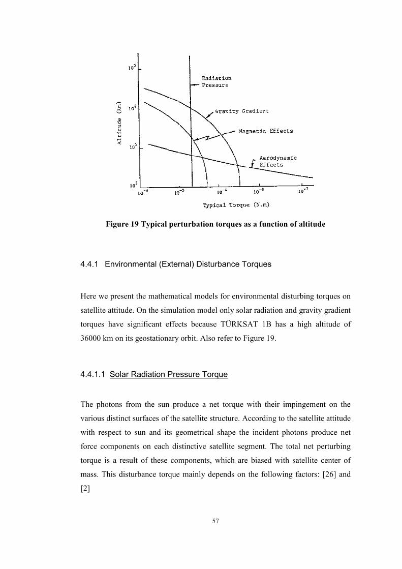
4.4.1 Environmental (External) Disturbance Torques ......................................................57
4.4.2 Internal Disturbance Torques ..................................................................................64
V. ATTITUDE CONTROL SYSTEM DESIGN..........................................................................66
5.1 PITCH CONTROL SYSTEM DESIGN.......................................................................................66
5.1.1 Equations for Pitch Motion ......................................................................................66
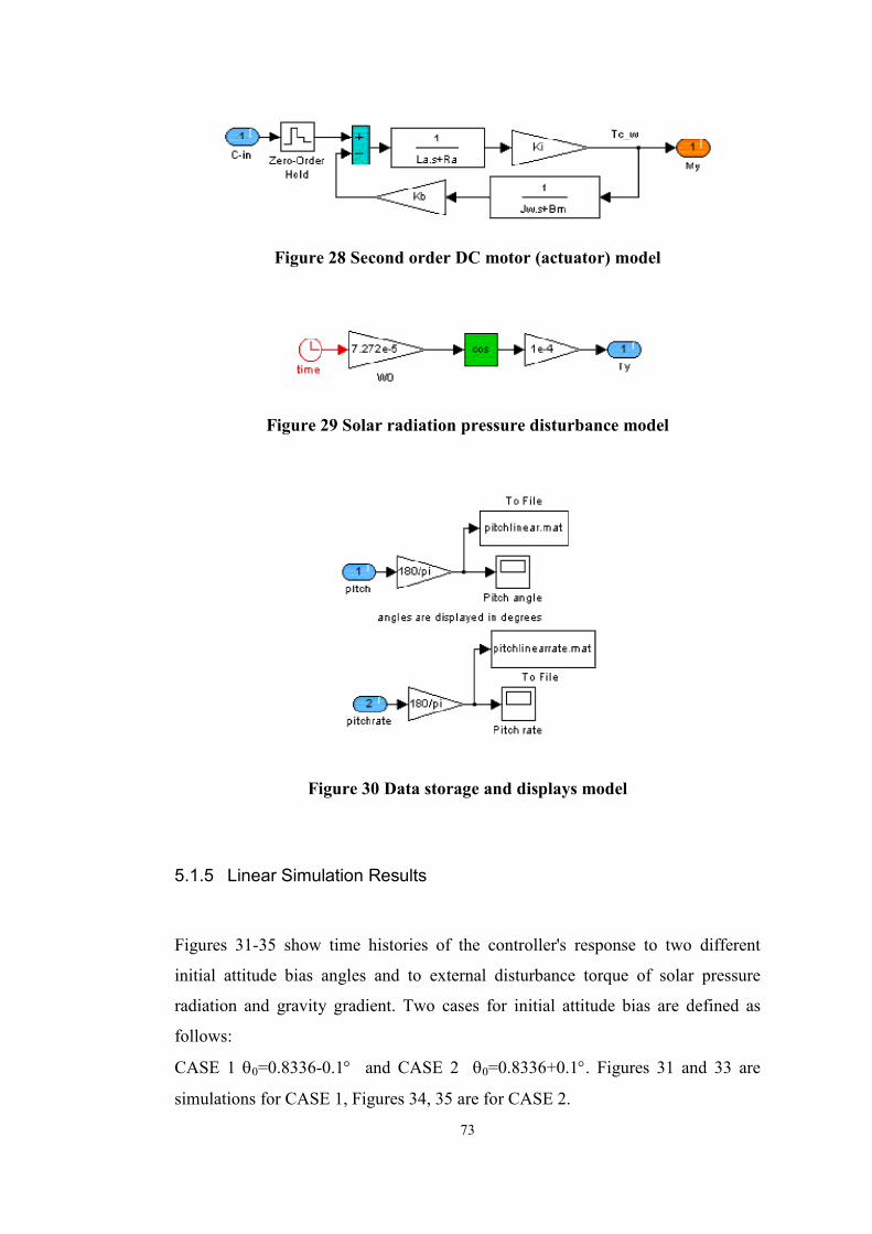
5.1.2 Actuator Model.........................................................................................................67
5.1.3 PD Controller Design: Tuning the Parameters........................................................70
5.1.4 Simulink Program for the Simulation of the Linear Pitch Dynamics Model, together
with the Controller..................................................................................................................71
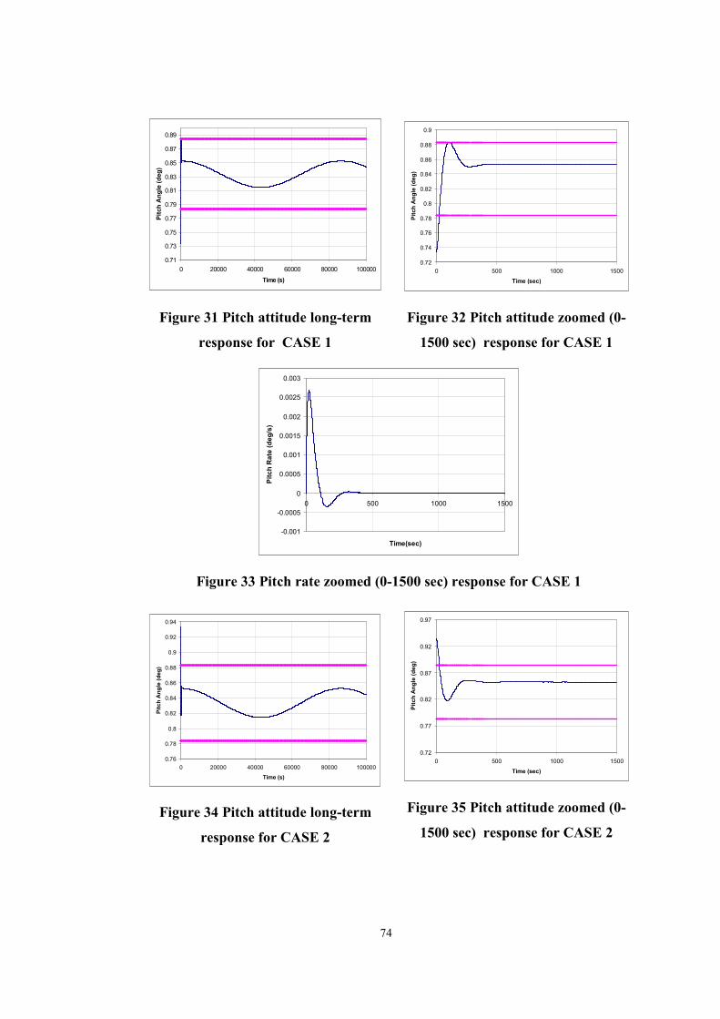
5.1.5 Linear Simulation Results.........................................................................................73
5.2 ROLL/YAW CONTROL SYSTEM DESIGN ..............................................................................75
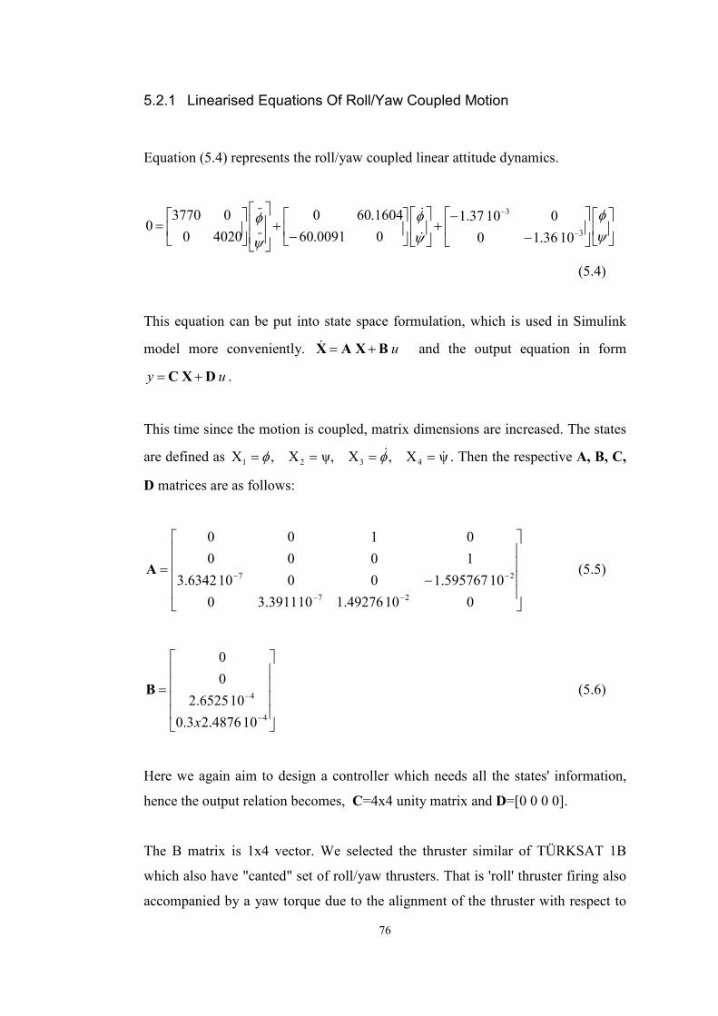
5.2.1 Linearised Equations Of Roll/Yaw Coupled Motion ................................................76
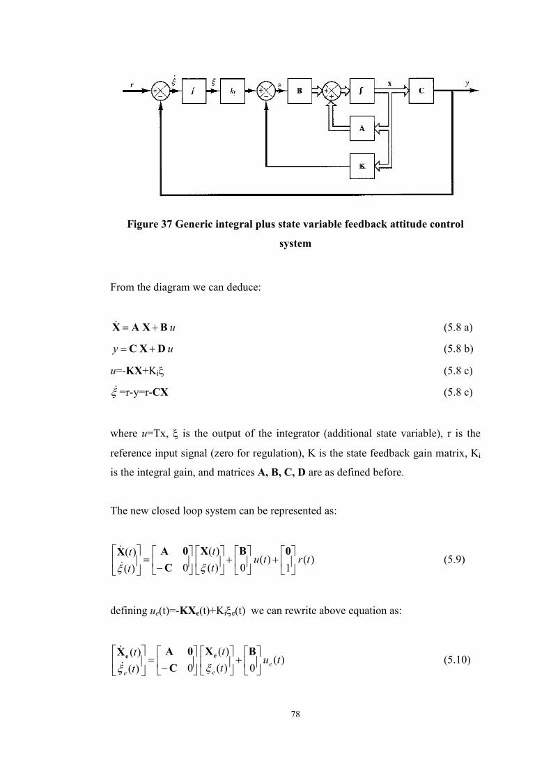
5.2.2 Controller Design for Coupled Linear Roll/Yaw Dynamics.....................................77
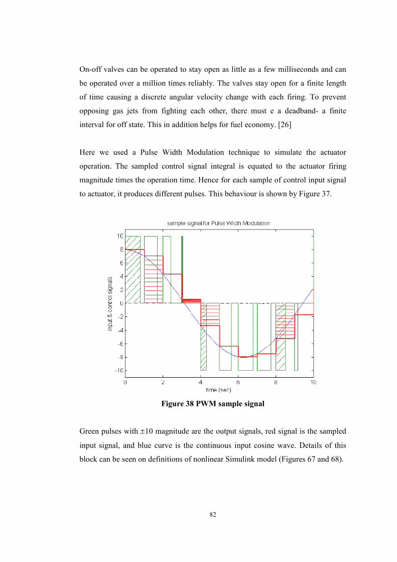
5.2.3 Thruster Model .........................................................................................................81
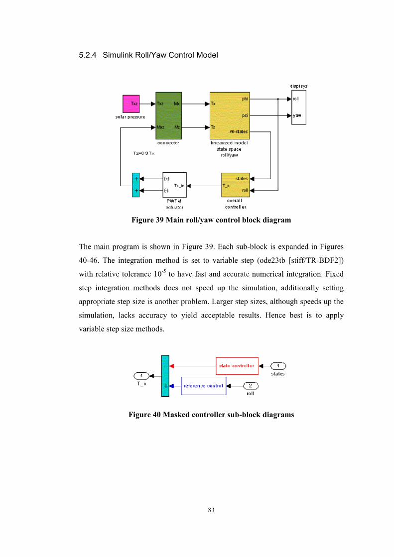
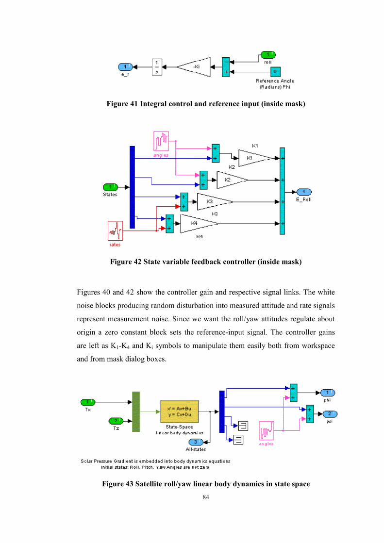
5.2.4 Simulink Roll/Yaw Control Model ............................................................................83
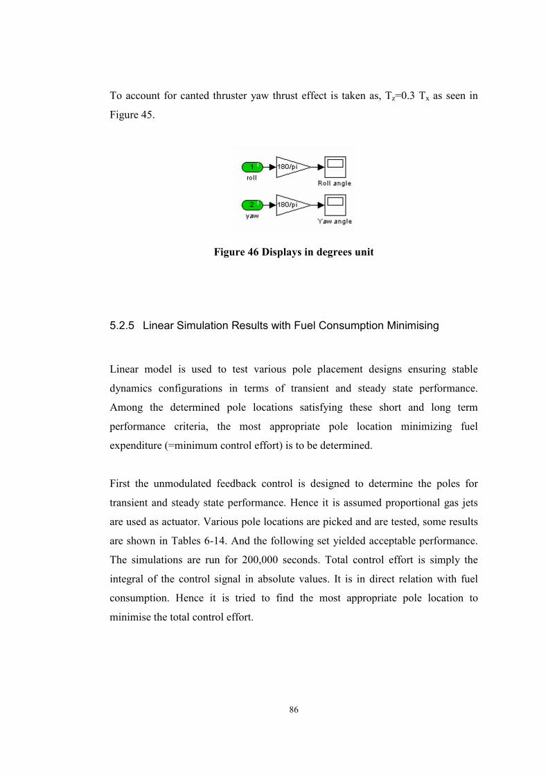
5.2.5 Linear Simulation Results with Fuel Consumption Minimising ...............................86
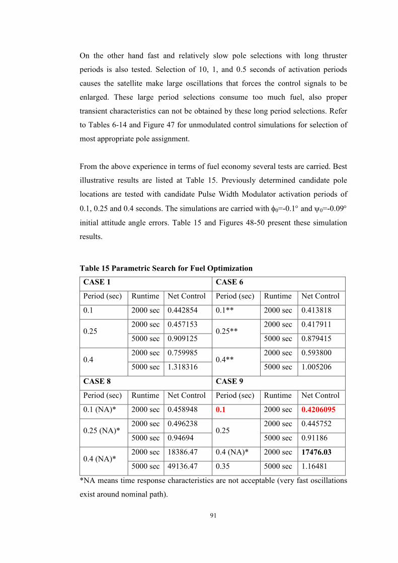
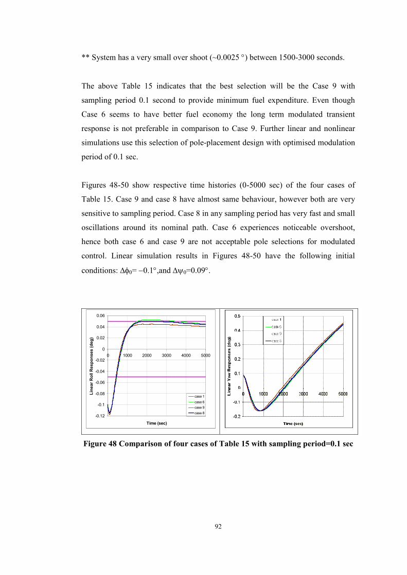
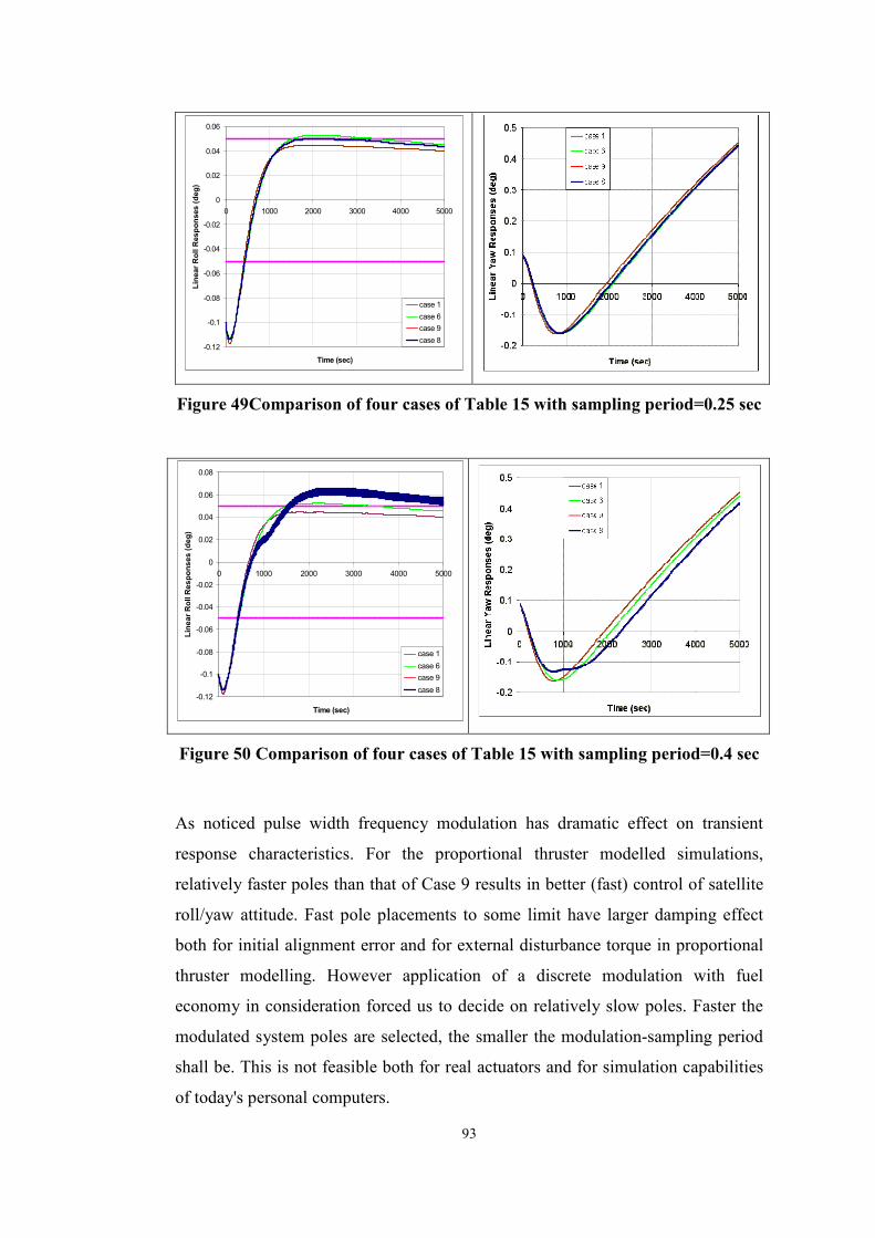
5.2.6 Linear Simulations with Pulse Width Modulated Actuator ......................................90
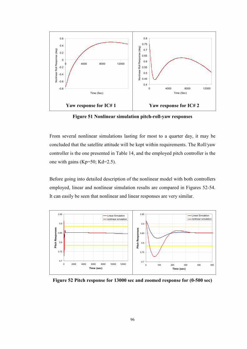
5.3 NONLINEAR SIMULATION ...................................................................................................94
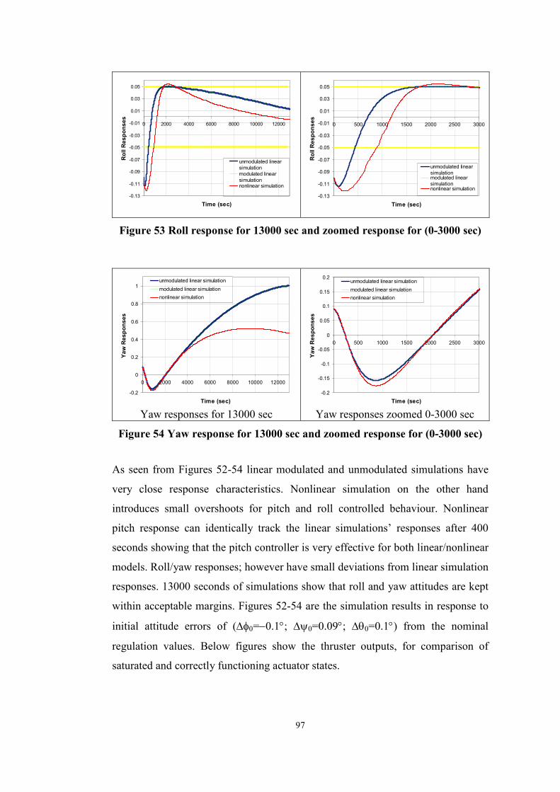
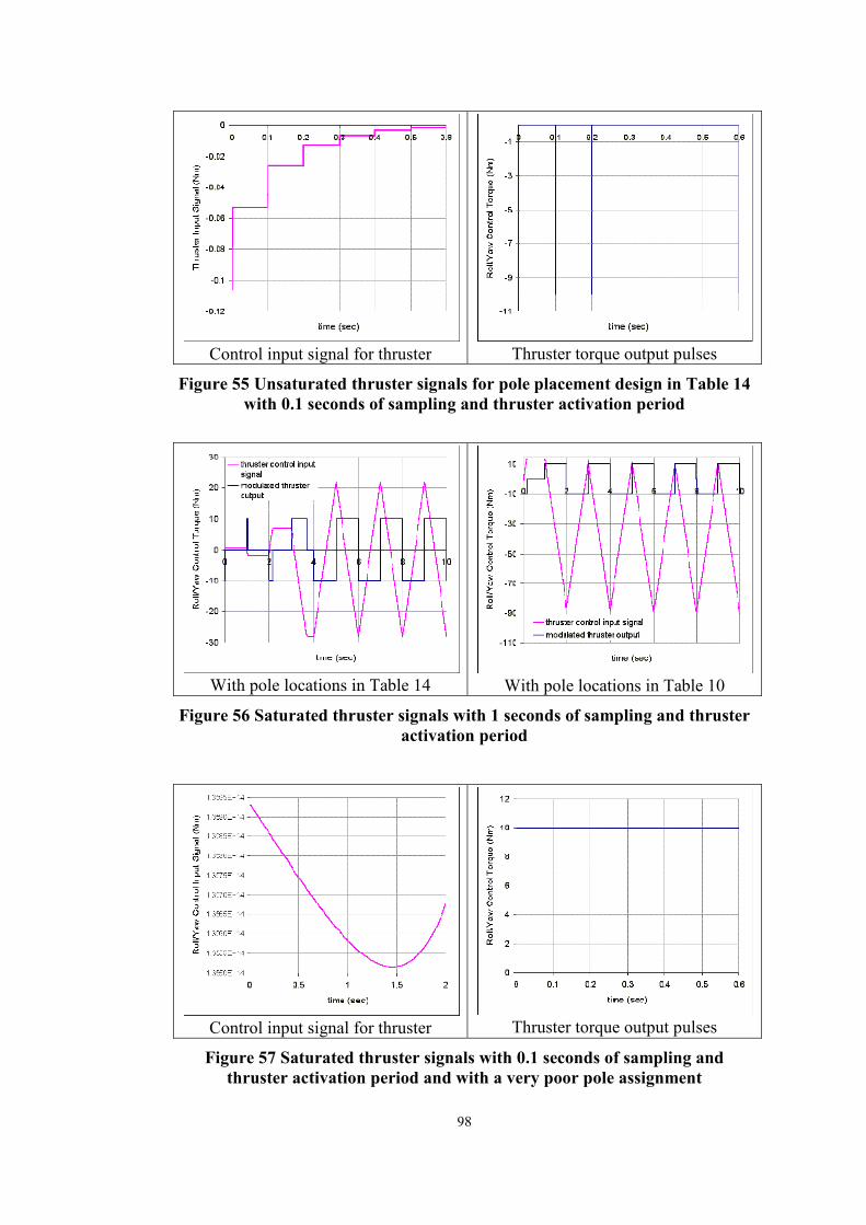
5.3.1 Nonlinear System Responses with Controllers .........................................................95
Page 7
vii
5.3.2 Description of Nonlinear Simulink Model with Controllers.....................................99
VI. SUMMARY AND CONCLUSION.......................................................................................104
REFERENCES .............................................................................................................................108
APPENDICES ....................................................................................................................................
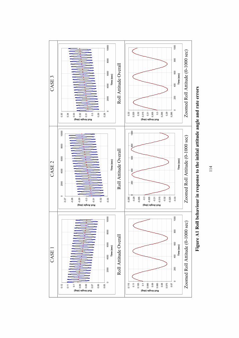
A. NONLINEAR BODY DYNAMICS BEHAVIOUR ANALYSES........................................112
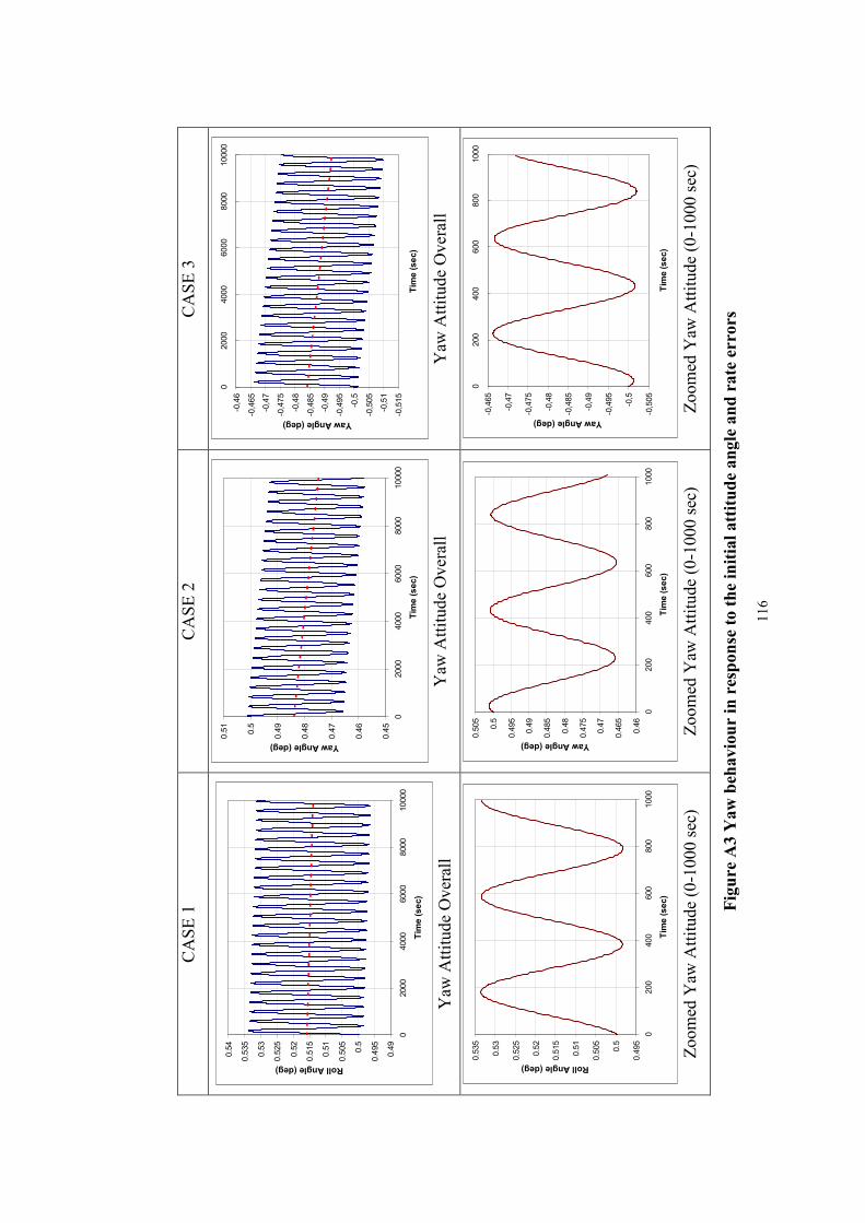
A.1. DISTURBANCE EFFECTS ARE EXCLUDED ....................................................................112
A.1.1. Simulations without the External Disturbance Torque...........................................112
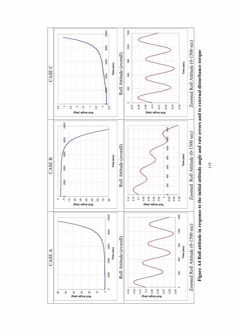
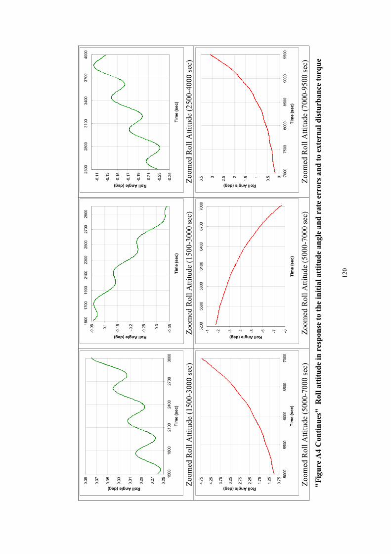
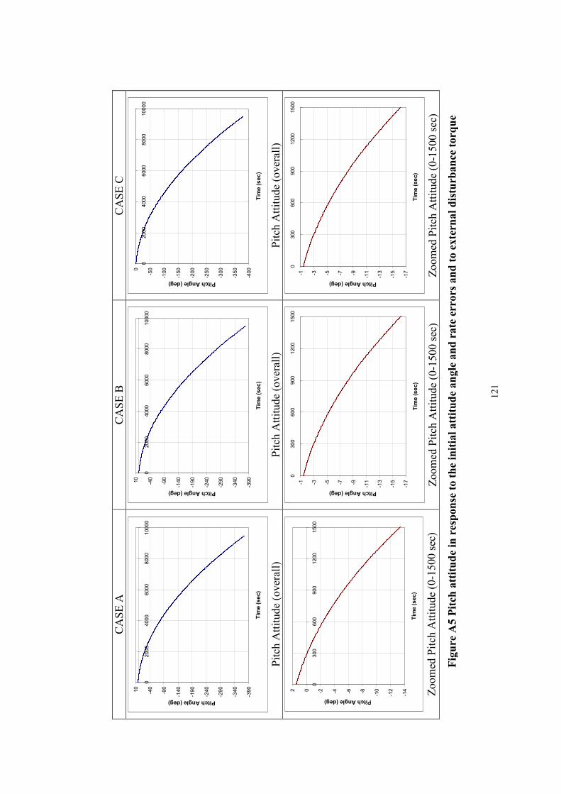
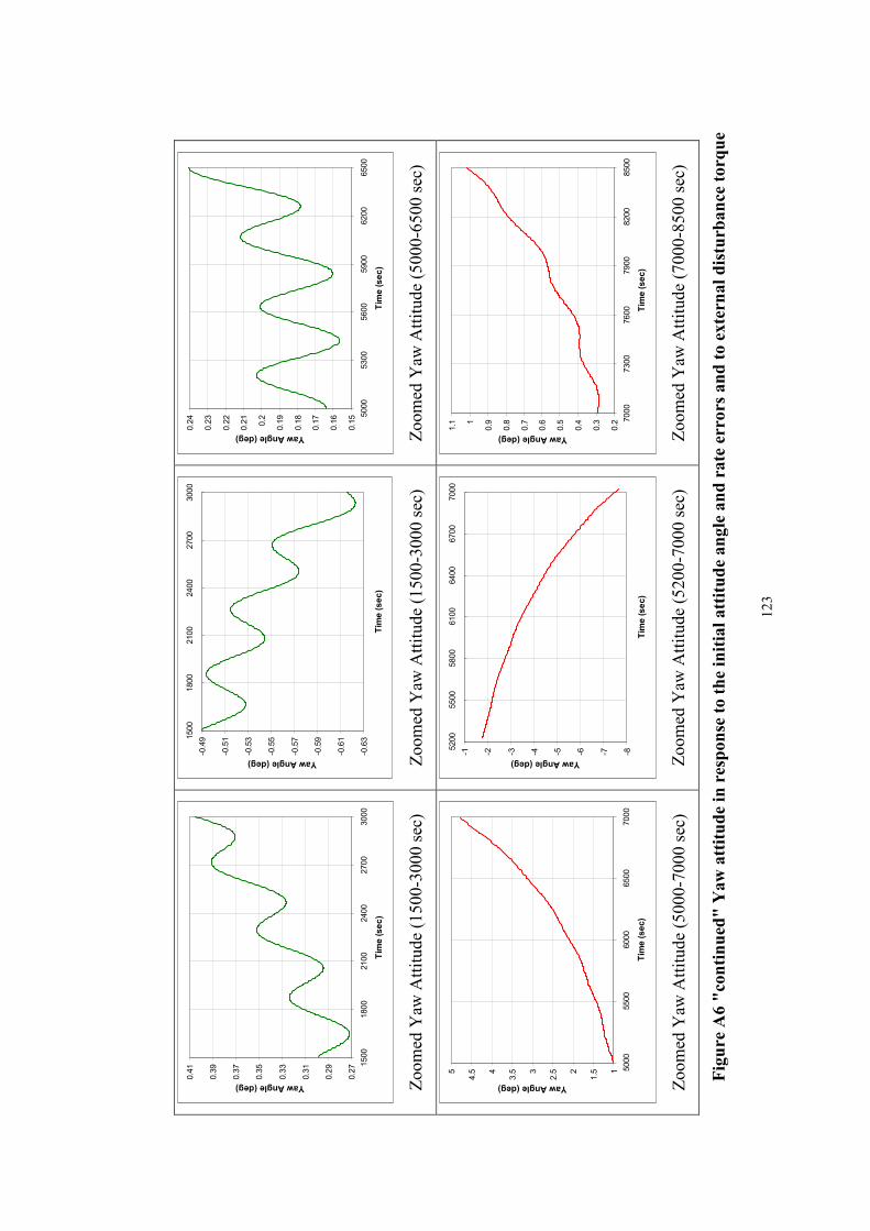
A.2. SIMULATIONS WITH DISTURBANCE TORQUE MODELS INCLUDED ................................117
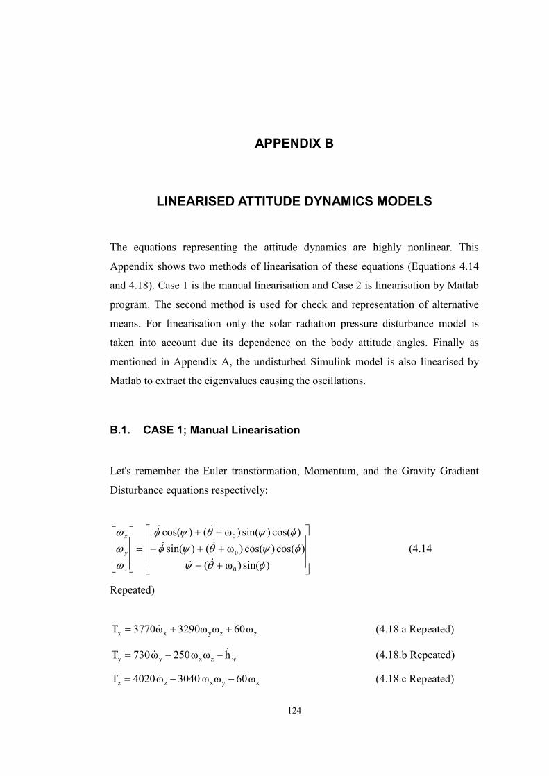
B. LINEARISED ATTITUDE DYNAMICS MODELS............................................................124
B.1. CASE 1; MANUAL LINEARISATION..............................................................................124
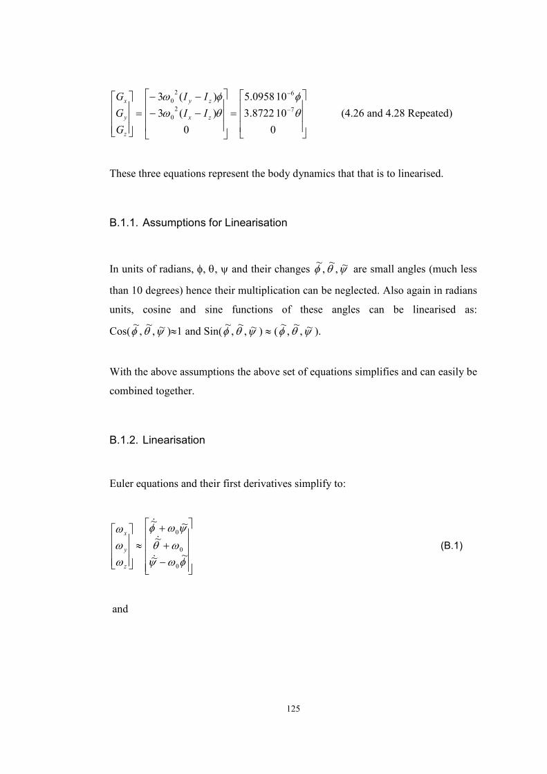
B.1.1. Assumptions for Linearisation................................................................................125
B.1.2. Linearisation ..........................................................................................................125
B.1.3. Stability Analysis ....................................................................................................128
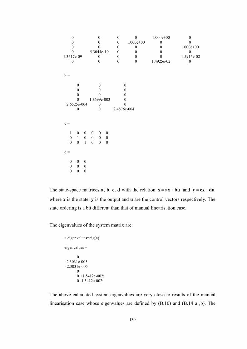
B.2. CASE 2; LINEARISATION BY MATLAB .........................................................................129
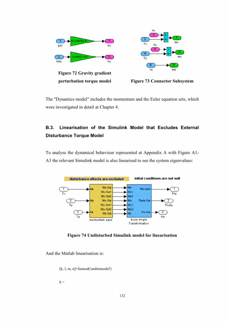
B.3. LINEARISATION OF THE SIMULINK MODEL THAT EXCLUDES EXTERNAL DISTURBANCE
TORQUE MODEL.........................................................................................................................132
B.4 SHORT DISCUSSION ON LINEARISATIONS IN TERMS OF STABILITY....................................134
Page 8
1
CHAPTER I
INTRODUCTION
1.1 Introduction to “Attitude Control of a Satellite Platform
Resembling to TÜRKSAT 1B”
Artificial satellites have become our everyday tools, just like our cars, televisions,
mobile phones, and so on. They are used for telecommunication, weather
forecasting, geological and interstellar surveys, for defense and spying applications
and many others. Mankind achieved to develop many types of artificial spacecraft
to satisfy the above indicated and many other needs: Micro satellites, low orbit,
high orbit or interstellar/interplanetary surveying satellites, geostationary and
special mission satellites like the GPS satellite group with service life varying
from weeks to decades. Many special or general use spacecraft are developed and
are being developed for a better understanding of the earth, close and far stellar
objects, the space and the human himself.
Turkey has also put his step in satellite communication business by TÜRKSAT
series of geostationary satellites. This increased Turkish scientists’ and engineers’
interest on spacecraft sciences like satellite communication; space vehicle’s orbit
and attitude dynamics, determination and control; celestial mechanics. TÜRKSAT
series of satellites brought a chance of technology transfer and development on
spacecraft sciences.
Determination of the satellite orbit is research area under celestial mechanics, a
branch of astrodynamics. Eskobal [1] define this as “the process of formulating a
Page 9
2
first approximation to the orbital parameters”. Astrodynamics in general deals with
the particle motion subject to a gravity field, such as body dynamics in the
interplanetary space. Celestial mechanics being a specific branch of it concentrates
on the natural motion of heavenly bodies.
The attitude dynamics of a spacecraft is another specific branch of astrodynamics.
This branch concentrates on the motion of the plant (the controlled space vehicle)
about its center of mass. [2] Naturally knowing attitude behaviour of the satellite
before production and placing on service orbit enable the designers to propose the
best control method to warrant its mission to be performed within specifications.
Here we notice two basic problems: Attitude / Motion dynamics determination and
proper control of the plant. This thesis work concentrates on spacecraft attitude
control.
TÜKSAT 1B, on its orbit continuously stay on specific latitude and longitude, and
pointed to earth to cover certain transmission area. These types of spacecraft are
placed on a geostationary orbit about 36000 to 42000 km away from earth. “A
geostationary satellite is subjected to various disturbances. As such it can not keep
its geostationary orbit and drifts from its required positions. Consequently, the
position and orbit parameters of the satellite must be corrected periodically by the
commands sent from a ground station. Orbit correction of TÜRKSAT 1B is
conducted from Gölbaşı and METU ground stations.” [3] Attitude correction is
done autonomously via the built in automatic control system of the satellite, the
ADCS (Attitude Determination and Control Sub-system). Orbit and attitude
control specifications are stringent for a telecommunication satellite to achieve its
mission. Space systems cost millions of US Dollars including launching, on orbit
servicing and the ground control services. Hence the modern space plants’
stability, robustness, reliability, tracking/pointing performance, service life and
other constraints have become more stringent in comparison to land/sea vehicle
systems and to previously designed space vehicles.
Introduction of modern control theory with various feasible techniques became
popular in spacecraft control problems as well. For example, gain scheduling, pole
Page 10
3
placement, Linear Quadratic Gaussian (LQG) techniques took attention mostly for
their robustness properties. [4] In real life the sensors are still noisy, plant
dynamics are still hard to model precisely, and the disturbances, as always, are still
existent. Various linear and nonlinear control methods are proposed to solve these
problems.
Development of electronics and computer sciences enabled faster and faster
onboard computing which led to more enhanced control strategies. A giant step in
digital control applications was realised by the introduction of online, discrete time
modeling of the process. This enabled many filtering (like Kalman Filter) and
plant prediction methods. Soon this was followed by the minimum variance
control (MVC) approach that is based on these prediction models under noisy
conditions. [5] These methods formed the background of optimization theory and
its control applications. [4]
Donald E. Kirk, at his book Optimal Control Theory; An Introduction, states the
basic differences between classical and optimal control theories as at the following
paragraph [6]:
Classical control system design is generally a trial-and-error process in which various
methods of analysis are used iteratively to determine the design parameters of an ‘’
acceptable’’ system. Acceptable performance is generally defined in terms of time
and frequency domain criteria such as rise time, settling time, peak overshoot, gain
and phase margin, and bandwidth. Radically different performance criteria must be
satisfied, however, by the complex, multiple-output systems required to meet the
demands of modern technology. For example, the design of a spacecraft attitude
control system that minimizes fuel expenditure is not amenable to solution by
classical methods. A new and direct approach to the synthesis of these complex
systems, called optimal control theory, has been made feasible by the development of
the digital computer.
The objective of optimal control theory is determine the control signals that will
cause a process to satisfy the physical constraints and at the same time minimize (or
maximize) some performance criterion.
Page 11
4
In this thesis Optimal Control problem is not addressed. However, the controller
sought for is desired to provide low fuel expenditure. Thus, we can state the
purpose of this thesis work completely; Design of a Control System for plant
model resembling to TÜRKSAT 1B satellite, with low fuel expenditure satisfying
various predefined attitude control constraints like keeping satellite pointing within
specified angle range. In shorter words this thesis is a study on “Attitude Control
of a Satellite Platform Resembling to TÜRKSAT 1B.” Controlled and
uncontrolled attitude behaviour of the satellite model is simulated via MATLAB-
Simulink software.
We shall briefly introduce our computing/modeling/simulating environment the
MATLAB 5.2: MATLAB is a technical computing environment for high-
performance numeric computation and visualization. MATLAB integrated
numerical analysis, matrix computation, signal processing, and graphics in an
easy-to-use environment where problems and solutions are expressed just as they
are written mathematically- without traditional programming. The name
MATLAB stands for Matrix Laboratory. MATLAB also features a family of
application-specific solutions called “toolboxes”. We will make use of
optimization and control system toolboxes and Nonlinear Control Design Blockset
of MATLAB during this thesis work. Finally we introduce the SIMULINK:
Simulink is a tool for modeling, analyzing and simulating a vast variety of
physical and mathematical systems, including those with nonlinear elements and
those which use continuous and discrete time. As an extension of MATLAB,
Simulink adds many features specific to dynamic systems while retaining all of
MATLAB’s general-purpose functionality. Using Simulink, we model a system
graphically, sidestepping much of the nuisance associated with conventional
programming.
A competitor program to MATLAB can be the MATRIX-X program, but unlike
MATLAB it is not so widely available to academic areas, and modeling with
MATRIX-X is more difficult in comparison with simple usage of Simulink.
Page 12
5
CHAPTER II
LITERATURE SURVEY
This section summarises the recent literature on attitude dynamics and control of
spacecraft. The publications from 1991 up to 1997 are compiled in this chapter.
The number of similar journals are very restricted, however most relative ones are
presented here.
2.1 Survey Summary
Liu and Singh [7] studied the fuel/time optimal control design of an inertially
symmetric spacecraft undergoing “rest-to-rest” maneuvers. They proposed both
time optimal and fuel/time optimal control problem solutions by a modified Switch
Time Optimization (STO) algorithm. Numerical STO algorithm integrates state
equations forward in time, and the costates (or adjoints) backward in time. Since
final time (tf) is set free and switching time depend on tf. Errors and final
constraints update iterative algorithm. Bang-off-Bang type control and optimal
number of switching are simulated. They used quaternion method to represent
body dynamics (state equations).
Similar to Liu & Singh, Bilimoira and Wie studied time optimal 3-axis control of
an inertially symmetric rigid spacecraft [8]. Time optimal solution is found to be
Bang-Bang type of control with optimal number of switching. Again quaternion
method is used to describe attitude dynamics of the spacecraft. Singular control
search yielded the necessity of saturation of at least one actuator. They simulated
the attitude behaviour by using a numerical approach: Multiple shooting algorithm
Page 13
6
with modified control constraint approach. Multiple shooting algorithm is for two-
point boundary value problems and is used with state-costate equations. Modified
control constraint approach is needed to determine control structure itself.
Minimum time 180° “rest-to-rest” maneuver control is simulated at the end of their
work.
Seywald et al. [9] present the fuel optimal solutions to reorient an inertially
symmetric rigid spacecraft from specified initial conditions to fully or partly
prescribed terminal conditions. First attitude dynamics are represented in terms of
quaternions, but in a different way than of Ref. [7] & Ref. [8] . They perform a
transformation on costate dynamics so that state-costate system dimension is
reduced. Defining the optimal control problem with related optimality conditions,
solutions for optimal and singular optimal control are investigated. Detailed
analysis for finite order and infinite order singular control is performed. Numerical
simulation results are presented at the end. Different from Ref. [7] & Ref. [8] they
present necessary conditions for numerical methods but selection of any particular
algorithm is left to the reader. Finally they compare all possible control logic.
Hablani [10] developed a pole placement technique to remove magnetic
disturbance torque from earth pointing spacecraft. Developed method is compared
with classical linear and Bang-Bang HxB control methods. (H: excess angular
momentum vector, B: geomagnetic field vector.) This technique is an alternative
method since magnetic momentum removal on some spacecraft can also be
managed by gravity gradient torque design.
Herman and Conway at their letter published in ‘Engineering notes’ [11] present
their work on the method of direct collocation and nonlinear programming which
is applied to the optimal control problem of satellite attitude control. Mission is to
recover a high orbit disabled satellite via a remotely operated satellite. The work
determines optimal open loop control histories for detumbling a disabled satellite.
The cost function becomes the integral square control, which is very similar to
well-known minimum energy performance index.
Page 14
7
J u u dtT
t
tf
= ∫1
20
( )B (2.1)
u: control vector, B: weighting matrix, t0: fixed, tf: free
Byrnes and Isidori investigated the existence of the smooth state feedback control
law, asymptotically stabilizing a rigid spacecraft with only two actuators
(thrusters) in operation [12]. It is shown that without any failure on the three
actuators state feedback law can asymptotically stabilize the system. EOM
(Equations of Motion) are defined by Euler’s equations. Additionally desired
control is derived using methods from a general nonlinear feedback design theory
with rootlocus study. They used topological methods to prove the related
theorems.
Pittelkau developed optimal control algorithms for autonomous magnetic roll/yaw
control of polar orbiting, earth oriented momentum bias spacecraft [13]. Optimal
design is required due periodic nature of roll/yaw dynamics. Linearized pitch
dynamics are developed from roll/yaw dynamics and found to be time invariant.
Design of a Linear Quadratic Gaussian (LQG) Control enabled disturbance
rejection. Including pitch control into performance index he suggests
J u R u x Qx dtTc
T
T
= +∫ ( )0
(2.2)
which can be solved by Ricatti differential equation numerically. The term xTQx
implies state feedback design and preceding term implies minimum energy
problem. State estimator design is solved via MATLAB. Simulation of closed loop
dynamics is presented at the end.
The paper by H. Weiss presents two-loop control of rate and attitude of a rigid
body [14]. The inner velocity loop controls the rate and the outer loop controls the
Page 15
8
angular position. The structure of a quaternion based rate/attitude tracking system
is presented with the discussion of the eigenaxis rotation in case of Proportional
(P) or Proportional + Integral (PI) error quaternion controllers. The stability of this
augmentation + attitude control system is studied. Finally he discusses application
of the proposed tracking system to gimbal attitude control.
The control problem solved by Nicosia and Tomei depends on measurement of
only angular positions [15]. In case of all the actuators are momentum wheels their
velocity measurements are also needed, to overcome this need they construct a
nonlinear observer by exploiting some structural properties of spacecraft model.
Spacecraft dynamics are represented by Euler angles. Then they derive a dynamic
output feedback controller and define a region of asymptotic stability. Finally they
design output feedback controller with reduced order estimator and simulate
results of observer, error dynamics, and controlled attitude dynamics.
Sun pressure produces significant effects on high altitudes like where
geostationary satellites are positioned. Venkatachalam proposes control of the
pitch attitude of a high altitude spacecraft by two-plate solar pressure controller as
the actuators [16]. No thruster activity is needed. He defines attitude and orbital
dynamics of unsymmetrical satellite with its center of mass moving in a circular
orbit about the earth center. He proposes simple output feedback controllers for
various values of final pitch angles and rates. The feedback constants are obtained
by solution of two-point boundary value problem. Also he studies the size effect of
the actuator on attitude dynamics.
Mathematical models of spacecraft dynamics are highly nonlinear and always
include idealizations. These handicaps prevent direct application of linear control
theory and also cause deviations from actual motion. Hence Lee et al. propose a
robust sliding-mode control law to handle not only the attitude reorientation
problem but also the tracking maneuver problem [17]. The two advantages of this
method are; first it can reject external disturbances, second it is robust to system
parameter changes. Spacecraft rigid body dynamics model is composed of two sets
of equations; the kinematics and dynamic equations in vector form. No frame
Page 16
9
transformation is used. Control law is designed with attitude dynamics on body
fixed frame. Lyapunov stability theory is used both for development and for
stability analysis of sliding mode control law. Robust control law is derived in two
consecutive steps. Finally simulations are performed to verify robustness and
appropriateness of control vector on a spacecraft mathematical model using only
thrusters as actuators.
Dodds and Walker propose sliding mode control for three-axis attitude control of a
rigid body spacecraft with unknown dynamics parameters [18]. They model
spacecraft dynamics in body coordinates only; using moment inertia matrix,
change of angular momentum magnitude and direction vectors and the kinematics
equations. Optical sensors and accelerometers do the attitude measurement.
Accelerations are directly measured, and angular rates and positions are estimated.
Only actuators are the tetrahedrally arranged reaction wheels. Actuator dynamics
are included the controller design but sensor dynamics are set undetermined.
Sliding control law comprises a linear state feedback section. Switching sequence
determination is performed. Finally simulation of controlled dynamics is
performed.
An adaptive control scheme to simulate the attitude and momentum management
of gravity gradient stabilized spacecraft is designed by Parlos and Sunkel [19].
Fully coupled nonlinear EOM are systematically linearized around an operating
point. Rigid body EOM (both orbital dynamics and attitude dynamics) is derived
in state space form. Only actuators are the momentum wheels. Gain scheduled
adaptive controller based on LQR (Linear Quadratic Regulator) design with pole
placement is proposed for attitude control of spacecraft undergoing mass
properties variations. Simulation results for a case study ‘Space Station Freedom’
are discussed in the final part.
Most common spacecraft attitude control method is the momentum management
via reaction wheels. Attitude error defines the control moment to be applied by the
actuators. When attitude errors are large systems show long term and large
oscillations. Piper and Kwatny show that matching nonlinear actuator dynamics
Page 17
10
(saturation) and controller dynamics (switches) properly, it is possible to reach a
globally stable equilibrium [20]. They uncouple pitch axis motion and design a
linear SISO (single input single output) pitch controller containing nonlinear
elements like switches. Proposed SISO controller is a simple PI controller when
pitch attitude error is below a threshold and a simple P when above the threshold.
It is shown that when actuators are saturated stability is lost.
Sharony and Meirovitch design an optimal controller for the control of
perturbations experienced by a spacecraft with a rigid hub and a flexible
appendage during minimum time maneuver [21]. Linear time varying set of
ordinary differential equations defines the model of vibration ad deviations from
rigid body EOM. Nonlinear two-point boundary value problem is encountered in
minimum time control formulation of nonlinear reduced order model. These yield
a different performance index, like:
J e z Sz e z Sz u Rut T t
ti
tf
T T= + +∫β β. . ( ) (2.3)
Where z: states, u: control, then the problem is converted into standard LQR
problem to be solved by Ricatti matrix equation via transformation z*(t)=eβtz(t).
The high orbit geosynchronous satellite three-axis stabilization is generally
achieved by using bias momentum wheels along the pitch axis. The paper by
Schwarzchild and Rajaran study on an attitude acquisition system for
geostationary satellites [22]. Main concern for us is the use of Euler angles and
quaternions for attitude acquisition control. The method uses direct rate quaternion
feedback to despin the spacecraft and to align the momentum wheel axis along the
orbit normal. Maneuver is designed to be performed along Euler axis.
Page 18
11
CHAPTER III
DESCRIPTION OF TÜRKSAT 1B SATELLITE SYSTEM WITH
A CONCENTRATION ON ATTITUDE CONTROL SUBSYSTEM
Procurement of TÜRKSAT series of satellites was initiated in 1989 by an
international contract led by Turkish PTT (now Turk Telecom). The French
Company Aerospatiale being a European consortium was contracted on December
1990 for the delivery of 2 satellites on orbit. This on orbit delivery also included
launching of satellites by Ariane rockets, delivery of 2 ground control stations,
providing support for operations, personnel training, program financing and
insurance. Aerospatiale’s shareholders for the program were:
From France: ALCATEL Escapce, Execorp, Arianespace
From Germany: MBB (DASA)
From Turkey: Teletaş –Alcatel Espace’s subsidiary
Both the ground stations are located in Ankara, major station in Gölbaşı and a
spare in METU campus.
3.1 TÜRKSAT 1-B On Orbit
Before starting detail descriptions at satellite system it’s better to summarize
phases and location of satellite itself was transformed to. On August 1994 it was
launched with Ariane rocket to 200-km altitude where is the perigee of its elliptical
transfer orbit. (Figure 1 [3]) The apogee point at the transfer orbit is 36000 km
distant to Earth. The next step was the firings of the apogee boost rocket of the
satellite with high thrust to move from transfer to drift orbit (near-synchronous
orbit). The small 10 N thrusters are activated to perform four manoeuvres to reach
the satellite’s service orbit -the geosynchronous or the geostationary orbit. There it
Page 19
12
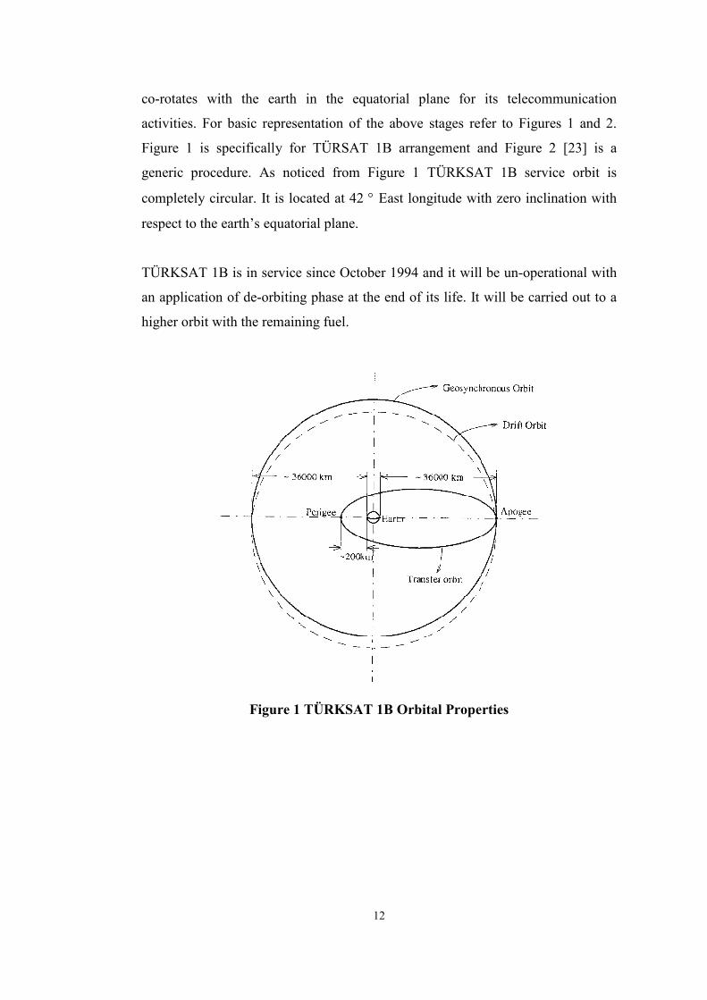
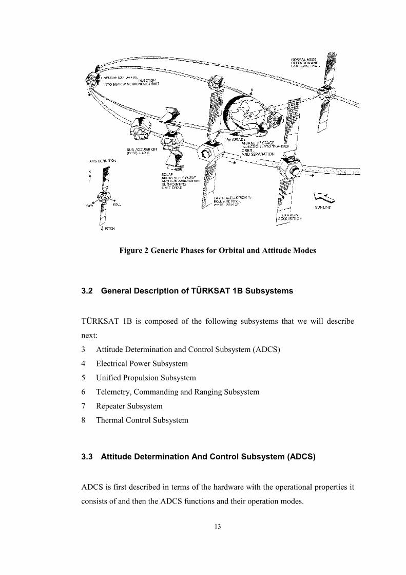
co-rotates with the earth in the equatorial plane for its telecommunication
activities. For basic representation of the above stages refer to Figures 1 and 2.
Figure 1 is specifically for TÜRSAT 1B arrangement and Figure 2 [23] is a
generic procedure. As noticed from Figure 1 TÜRKSAT 1B service orbit is
completely circular. It is located at 42 ° East longitude with zero inclination with
respect to the earth’s equatorial plane.
TÜRKSAT 1B is in service since October 1994 and it will be un-operational with
an application of de-orbiting phase at the end of its life. It will be carried out to a
higher orbit with the remaining fuel.
Figure 1 TÜRKSAT 1B Orbital Properties
Page 20
13
Figure 2 Generic Phases for Orbital and Attitude Modes
3.2 General Description of TÜRKSAT 1B Subsystems
TÜRKSAT 1B is composed of the following subsystems that we will describe
next:
3 Attitude Determination and Control Subsystem (ADCS)
4 Electrical Power Subsystem
5 Unified Propulsion Subsystem
6 Telemetry, Commanding and Ranging Subsystem
7 Repeater Subsystem
8 Thermal Control Subsystem
3.3 Attitude Determination And Control Subsystem (ADCS)
ADCS is first described in terms of the hardware with the operational properties it
consists of and then the ADCS functions and their operation modes.
Page 21
14
TÜRKSAT 1B ADCS is an optimized combination of the necessary (most are
redundantly coupled) hardware and relevant software for autonomous or ground
controlled manoeuvring. Its main mission is to maintain the spacecraft’s attitude
within its specifications. Sun and earth sensors assemblies, rate integrated gyro
assembly provide signals to determine the current attitude of the space vehicle and
the actuators (hydrazine thrusters and momentum wheels) act under ADCS’s
command to manoeuvre the satellite to rearrange its attitude.
During most of the satellite service life ADCS is responsible from on station
antenna pointing by station keeping manoeuvres. Another task assigned to ADCS
is the transmission of systems monitoring data to ground stations through the
Telemetry, Commanding and ranging Subsystem. [24]
Next we will introduce the ADCS hardware (sensors, actuators, and so on) then
their functionality will be described by ADCS mission descriptions by various
satellite operation modes.
TÜRKSAT 1B ADCS Hardware Configuration described in detail through section
3.3.1 to section 3.3.4
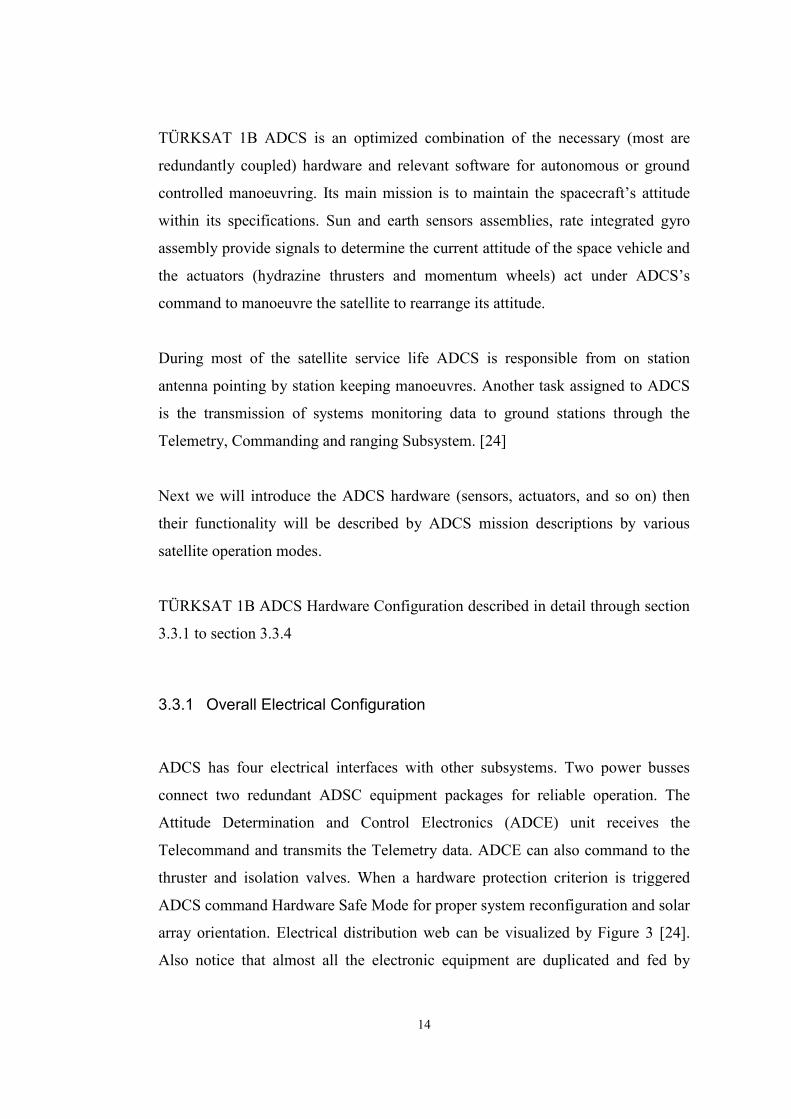
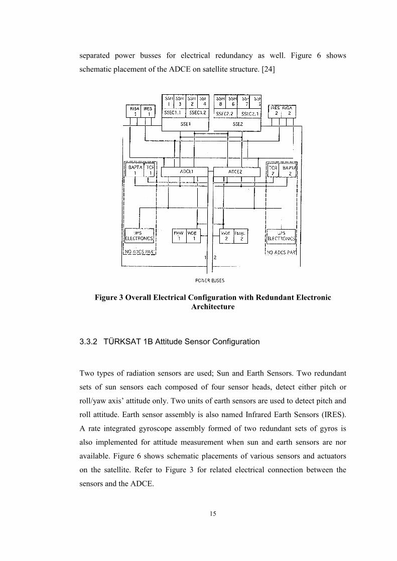
3.3.1 Overall Electrical Configuration
ADCS has four electrical interfaces with other subsystems. Two power busses
connect two redundant ADSC equipment packages for reliable operation. The
Attitude Determination and Control Electronics (ADCE) unit receives the
Telecommand and transmits the Telemetry data. ADCE can also command to the
thruster and isolation valves. When a hardware protection criterion is triggered
ADCS command Hardware Safe Mode for proper system reconfiguration and solar
array orientation. Electrical distribution web can be visualized by Figure 3 [24].
Also notice that almost all the electronic equipment are duplicated and fed by
Page 22
15
separated power busses for electrical redundancy as well. Figure 6 shows
schematic placement of the ADCE on satellite structure. [24]
Figure 3 Overall Electrical Configuration with Redundant Electronic Architecture
3.3.2 TÜRKSAT 1B Attitude Sensor Configuration
Two types of radiation sensors are used; Sun and Earth Sensors. Two redundant
sets of sun sensors each composed of four sensor heads, detect either pitch or
roll/yaw axis’ attitude only. Two units of earth sensors are used to detect pitch and
roll attitude. Earth sensor assembly is also named Infrared Earth Sensors (IRES).
A rate integrated gyroscope assembly formed of two redundant sets of gyros is
also implemented for attitude measurement when sun and earth sensors are nor
available. Figure 6 shows schematic placements of various sensors and actuators
on the satellite. Refer to Figure 3 for related electrical connection between the
sensors and the ADCE.
Page 23
16
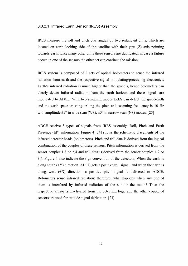
3.3.2.1 Infrared Earth Sensor (IRES) Assembly
IRES measure the roll and pitch bias angles by two redundant units, which are
located on earth looking side of the satellite with their yaw (Z) axis pointing
towards earth. Like many other units these sensors are duplicated, in case a failure
occurs in one of the sensors the other set can continue the mission.
IRES system is composed of 2 sets of optical bolometers to sense the infrared
radiation from earth and the respective signal modulating/processing electronics.
Earth’s infrared radiation is much higher than the space’s, hence bolometers can
clearly detect infrared radiation from the earth horizon and these signals are
modulated to ADCE. With two scanning modes IRES can detect the space-earth
and the earth-space crossing. Along the pitch axis-scanning frequency is 10 Hz
with amplitude ±9° in wide scan (WS), ±5° in narrow scan (NS) modes. [25]
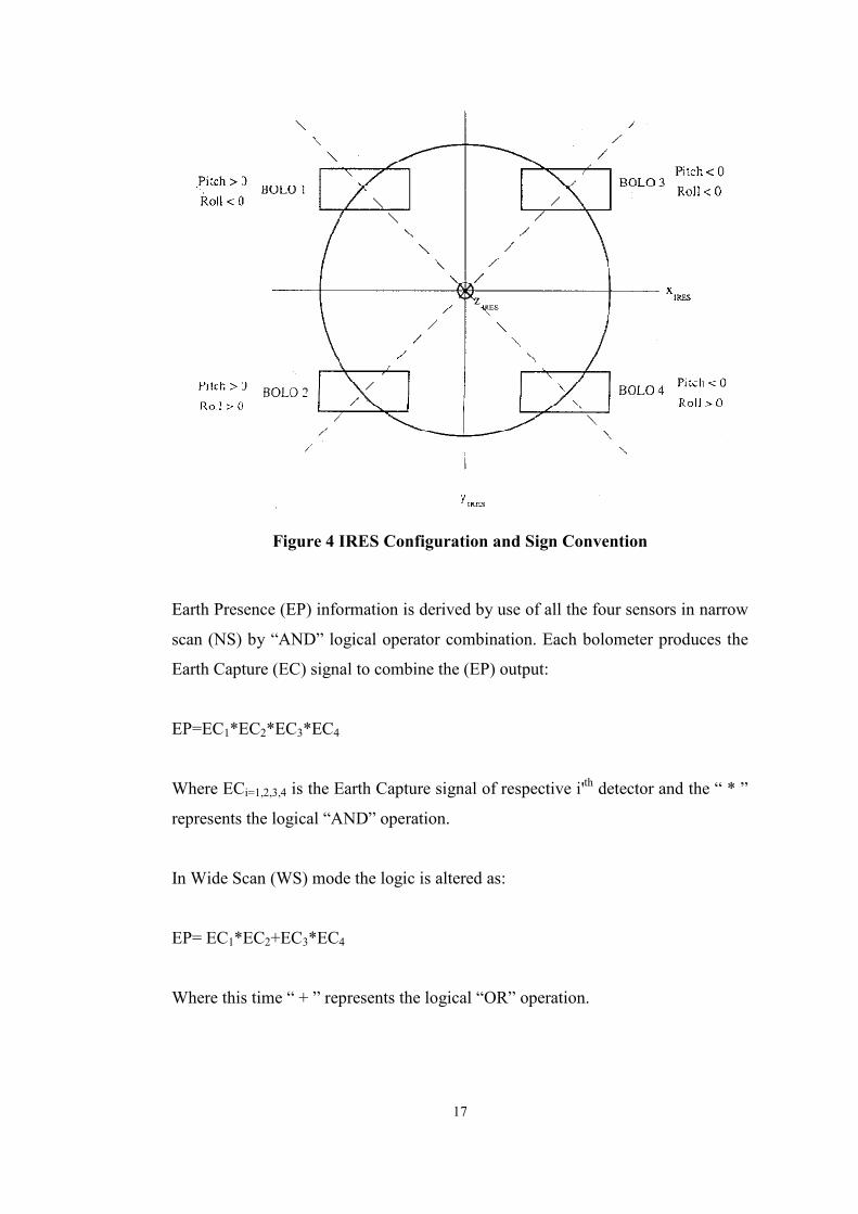
ADCE receive 3 types of signals from IRES assembly; Roll, Pitch and Earth
Presence (EP) information. Figure 4 [24] shows the schematic placements of the
infrared detector heads (bolometers). Pitch and roll data is derived from the logical
combination of the couples of these sensors: Pitch information is derived from the
sensor couples 1,3 or 2,4 and roll data is derived from the sensor couples 1,2 or
3,4. Figure 4 also indicate the sign convention of the detectors; When the earth is
along south (+Y) direction, ADCE gets a positive roll signal, and when the earth is
along west (+X) direction, a positive pitch signal is delivered to ADCE.
Bolometers sense infrared radiation; therefore, what happens when any one of
them is interfered by infrared radiation of the sun or the moon? Then the
respective sensor is inactivated from the detecting logic and the other couple of
sensors are used for attitude signal derivation. [24]
Page 24
17
Figure 4 IRES Configuration and Sign Convention
Earth Presence (EP) information is derived by use of all the four sensors in narrow
scan (NS) by “AND” logical operator combination. Each bolometer produces the
Earth Capture (EC) signal to combine the (EP) output:
EP=EC1*EC2*EC3*EC4
Where ECi=1,2,3,4 is the Earth Capture signal of respective i'th detector and the “ * ”
represents the logical “AND” operation.
In Wide Scan (WS) mode the logic is altered as:
EP= EC1*EC2+EC3*EC4
Where this time “ + ” represents the logical “OR” operation.
Page 25
18
WS mode is selected when earth acquisition has not been established and is to be
reached. NS mode is selected when the earth acquisition is already established.
Naturally this mode provides more accurate data. [3]
3.3.2.2 Sun Sensor Assembly (SSA)
Similar to the earth sensor assembly, SSA is composed of two sets of Sun Sensor
Heads and two separate Sun Sensor Electronics (SSE). [25] Each set of SSH is
composed of 4 detectors located on the spacecraft structure with different view
angles. Studying Figure 5 [3] we notice those 2 sets of SSH combined with two
redundant SSE Channels (SSEC) from a 4x4 redundant SSA architecture. Four of
the SSH are for nominal usage the rest is the back up. SSA control logic includes
switching operations. SSEC activates one SSH by switching on, hence operation of
a SSH requires a multi-step operation. Physical location of the SSH couple
determine which pair is to be activated during manoeuvre phase. After appropriate
pair is switched on, one of the SSH of the enabled pair is selected for angle
computation.
The signals produced by SSA are proportional to the out of and in plane of the
spacecraft sun vector. SSH 1 and 5 determine the out of plane component and the
rest derive the in plane vector. These two signals are used to compute the yaw/roll
deviations of the satellite attitude. Nominal SSH are the ones on the left (SSE1) of
the Figure 5 and the ones at the right side are backup. SSA is not used during
nominal operation, because spacecraft attitude is kept with control application on
pitch and roll axis only, and the IRES provide information for these angles’ bias.
On the other hand for relatively more critical manoeuvres like station keeping, yaw
angle needs to be crosschecked. Therefore, a SSH is activated for the on-board
yaw angle computation. SSH can scan an area of ±60 ° with 0.05 ° resolution and
0.063 ° accuracy. Figure 6 shows the schematic placement of the SSE on satellite.
[24]
Page 26
19
Figure 5 Sun Sensor Operation Logic
3.3.2.3 Rate Integrated Gyro Assembly (RIGA)
RIGA is composed of two redundant three-axis gyroscope packages, which
measure the angular rates of the satellite rotation and angular motion with respect
to the universal reference frame. Each gyro unit is formed of three gyroscopes with
associated electronics. They produce analog output signals in the form of pulse
trains for each control axis. The two separate RIGAs are located on north panel of
the satellite. And are kept in OFF mode during normal mode. RIGA because of its
error growth nature, it needs calibration regularly. Hence they are used when IRES
or SSA can not be relied on. Another problem with RIGA is that, its performance
highly depends on how stable the RIGA temperature is. Sudden changes in its
temperature cause it to produce more erroneous signals. RIGA’s linear range is
limited to ±2°/s and has a pulse train of 1 second. ADCE use a clock time of 100
ms; therefore, pulse trains are counted at 10 Hz Frequency. Figure 6 shows the
schematic placement of the assembly on the satellite structure. Figure 3 shows the
electrical connection between the RIGA and the ADCE. [24]
3.3.3 Attitude Determination and Control Electronics
Page 27
20
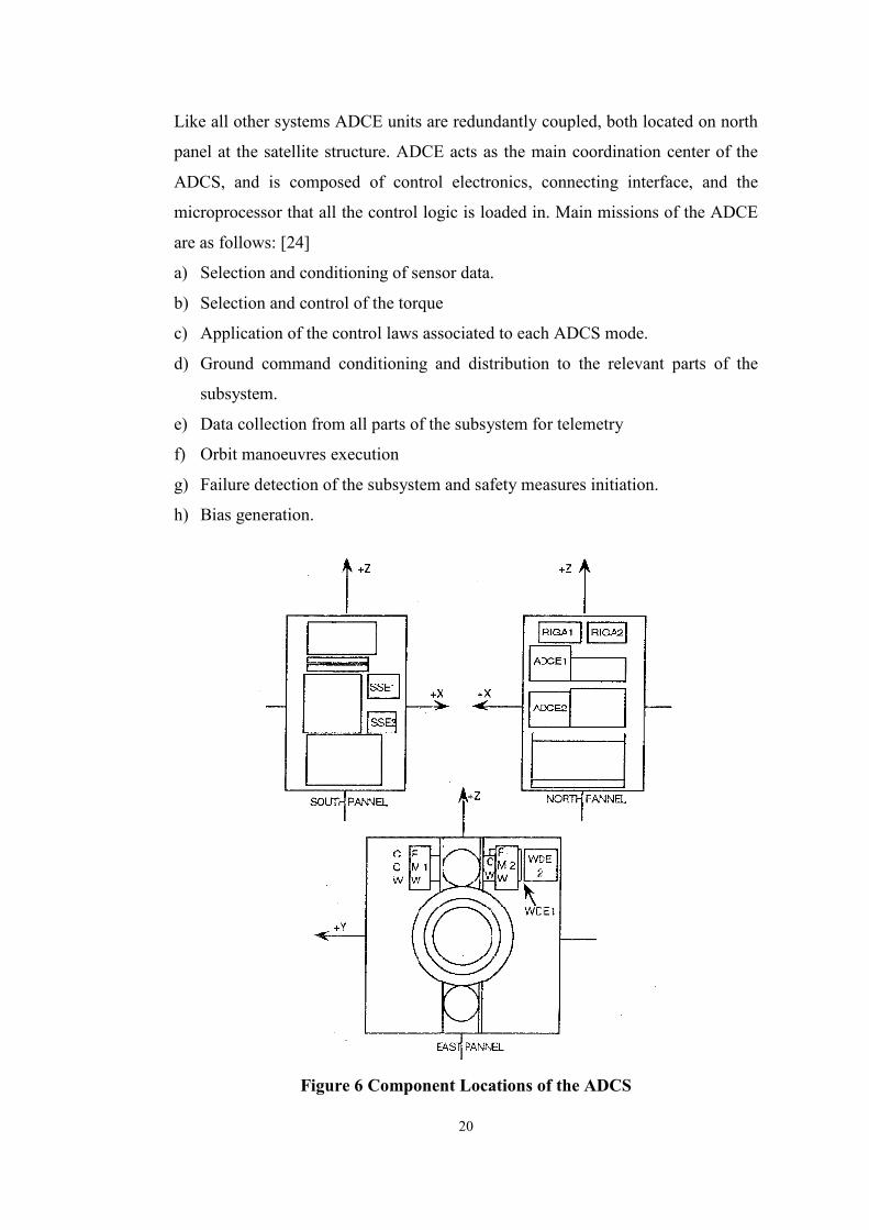
Like all other systems ADCE units are redundantly coupled, both located on north
panel at the satellite structure. ADCE acts as the main coordination center of the
ADCS, and is composed of control electronics, connecting interface, and the
microprocessor that all the control logic is loaded in. Main missions of the ADCE
are as follows: [24]
a) Selection and conditioning of sensor data.
b) Selection and control of the torque
c) Application of the control laws associated to each ADCS mode.
d) Ground command conditioning and distribution to the relevant parts of the
subsystem.
e) Data collection from all parts of the subsystem for telemetry
f) Orbit manoeuvres execution
g) Failure detection of the subsystem and safety measures initiation.
h) Bias generation.
Figure 6 Component Locations of the ADCS
Page 28
21
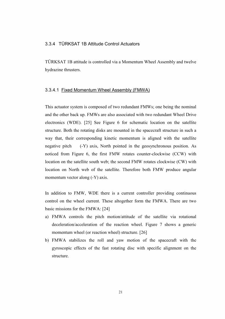
3.3.4 TÜRKSAT 1B Attitude Control Actuators
TÜRKSAT 1B attitude is controlled via a Momentum Wheel Assembly and twelve
hydrazine thrusters.
3.3.4.1 Fixed Momentum Wheel Assembly (FMWA)
This actuator system is composed of two redundant FMWs; one being the nominal
and the other back up. FMWs are also associated with two redundant Wheel Drive
electronics (WDE). [25] See Figure 6 for schematic location on the satellite
structure. Both the rotating disks are mounted in the spacecraft structure in such a
way that, their corresponding kinetic momentum is aligned with the satellite
negative pitch (-Y) axis, North pointed in the geosynchronous position. As
noticed from Figure 6, the first FMW rotates counter-clockwise (CCW) with
location on the satellite south web; the second FMW rotates clockwise (CW) with
location on North web of the satellite. Therefore both FMW produce angular
momentum vector along (-Y) axis.
In addition to FMW, WDE there is a current controller providing continuous
control on the wheel current. These altogether form the FMWA. There are two
basic missions for the FMWA: [24]
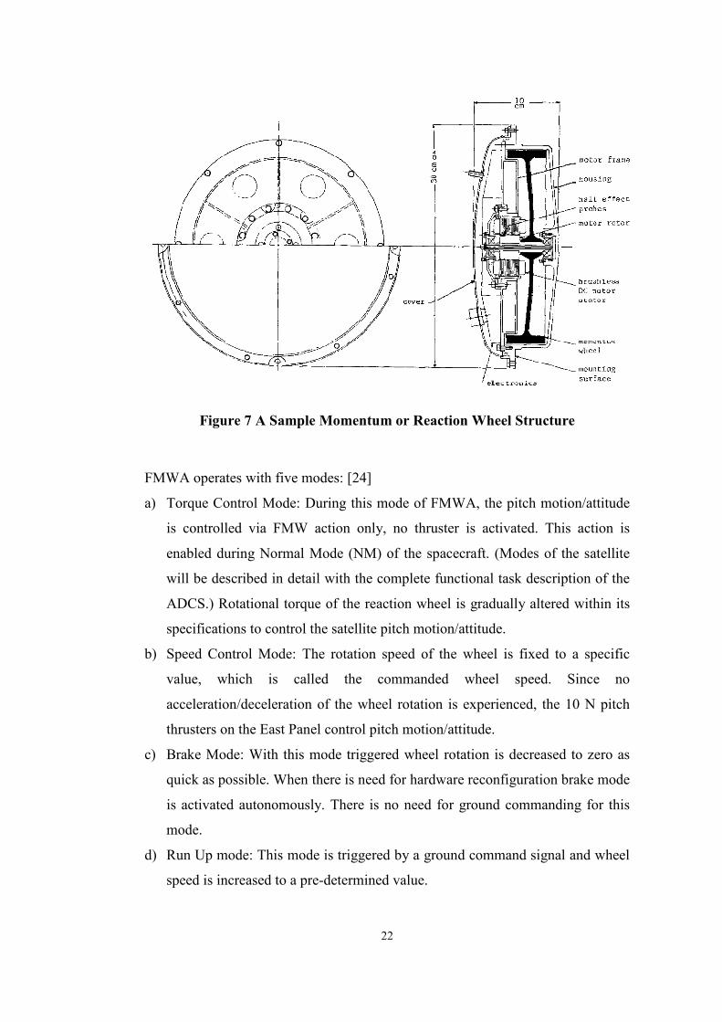
a) FMWA controls the pitch motion/attitude of the satellite via rotational
deceleration/acceleration of the reaction wheel. Figure 7 shows a generic
momentum wheel (or reaction wheel) structure. [26]
b) FMWA stabilizes the roll and yaw motion of the spacecraft with the
gyroscopic effects of the fast rotating disc with specific alignment on the
structure.
Page 29
22
Figure 7 A Sample Momentum or Reaction Wheel Structure
FMWA operates with five modes: [24]
a) Torque Control Mode: During this mode of FMWA, the pitch motion/attitude
is controlled via FMW action only, no thruster is activated. This action is
enabled during Normal Mode (NM) of the spacecraft. (Modes of the satellite
will be described in detail with the complete functional task description of the
ADCS.) Rotational torque of the reaction wheel is gradually altered within its
specifications to control the satellite pitch motion/attitude.
b) Speed Control Mode: The rotation speed of the wheel is fixed to a specific
value, which is called the commanded wheel speed. Since no
acceleration/deceleration of the wheel rotation is experienced, the 10 N pitch
thrusters on the East Panel control pitch motion/attitude.
c) Brake Mode: With this mode triggered wheel rotation is decreased to zero as
quick as possible. When there is need for hardware reconfiguration brake mode
is activated autonomously. There is no need for ground commanding for this
mode.
d) Run Up mode: This mode is triggered by a ground command signal and wheel
speed is increased to a pre-determined value.
Page 30
23
e) Run Down Mode: Similarly wheel speed is reduced to a pre-selected value by
a ground telecommand.
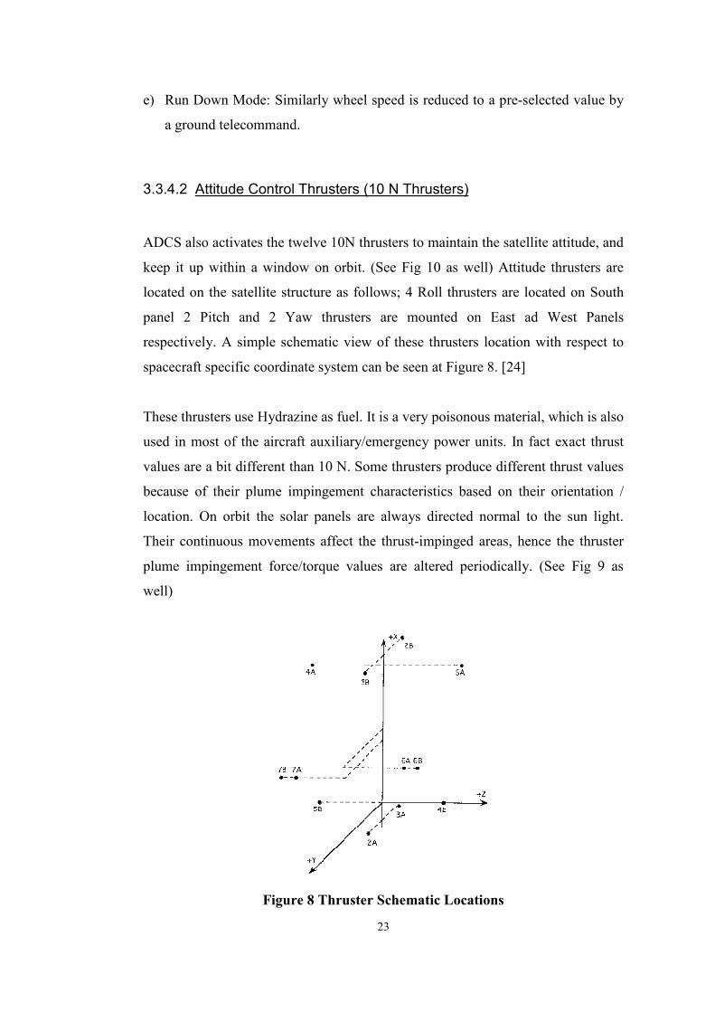
3.3.4.2 Attitude Control Thrusters (10 N Thrusters)
ADCS also activates the twelve 10N thrusters to maintain the satellite attitude, and
keep it up within a window on orbit. (See Fig 10 as well) Attitude thrusters are
located on the satellite structure as follows; 4 Roll thrusters are located on South
panel 2 Pitch and 2 Yaw thrusters are mounted on East ad West Panels
respectively. A simple schematic view of these thrusters location with respect to
spacecraft specific coordinate system can be seen at Figure 8. [24]
These thrusters use Hydrazine as fuel. It is a very poisonous material, which is also
used in most of the aircraft auxiliary/emergency power units. In fact exact thrust
values are a bit different than 10 N. Some thrusters produce different thrust values
because of their plume impingement characteristics based on their orientation /
location. On orbit the solar panels are always directed normal to the sun light.
Their continuous movements affect the thrust-impinged areas, hence the thruster
plume impingement force/torque values are altered periodically. (See Fig 9 as
well)
Figure 8 Thruster Schematic Locations
Page 31
24
Thrusters 6A, 6B, 7A, 7B are the South thrusters. 2B, 3B, 4A and 5A are the East
thrusters and the rest are the West thrusters.
Thrusters are not affected from center of gravity shift during satellite life; therefore
nominal thrust values during (BOT and EOT) also during (BOL and EOL) are
identical. (BOT: Beginning of Transfer, EOT: End of Transfer, BOL: Beginning of
Life; EOL: End of Life). There is no west reflector hence west (yaw) thrusters are
not subject to an impingement distortion from 10N nominal thrust. On the other
hand both the pitch thrusters on East Panel the roll thrusters on South Panel
experience minor impingement thrust alterations during BOT (=EOT) and BOL
(=EOL) due to solar panels, antennas and other geometrical surfaces of the
structure. During service life (Geostationary Orbit) Solar panel is continuously
kept normal to the sunrays hence roll-thrusters also periodically (twice a day)
experience additional distortions. Each hour with twice a day periodicity
impingement forces / torques are altered. However on transfer orbit sun panels are
not fully employed hence south thrusters do not experience this periodicity
between BOT–EOT. In general in comparison to 10N nominal thrust impingement
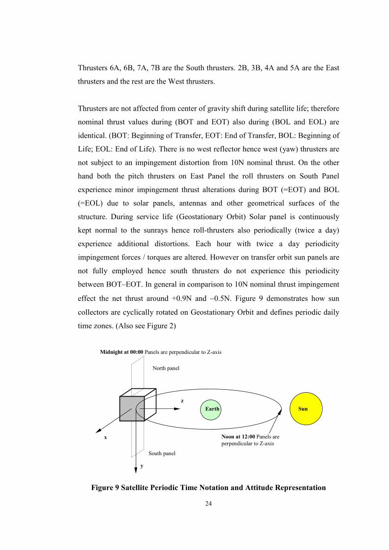
effect the net thrust around +0.9N and −0.5N. Figure 9 demonstrates how sun
collectors are cyclically rotated on Geostationary Orbit and defines periodic daily
time zones. (Also see Figure 2)
Sun
South panel
z
Earth
North panel
x
y
Midnight at 00:00 Panels are perpendicular to Z-axis
Noon at 12:00 Panels areperpendicular to Z-axis
Figure 9 Satellite Periodic Time Notation and Attitude Representation
Page 32
25
The thruster nozzle exits are not aligned in accordance with the satellite body axes
rather all are given various bias angles (all are not symmetric). Defining XT, YT,
and ZT as the nozzle exit plane center in the spacecraft axis system, nozzles are
biased with α as the nominal angle of the thruster aligned in XY plane, and with β
as the nominal thruster angle out of XY plane. Studying the roll thrusters’
alignment it is seen that the nominal 10 N force is divided into 3 components in X-
Y-Z directions. [24]
Functions of TÜRKSAT 1B ADCS at its various segments on orbit and service life
and its respective operation modes are described in detail through the following
sections:
3.3.5 Functions of the ADCS during Transfer Orbit (TO)
TÜRKSAT 1B ADCS missions during Transfer Orbit (TO) phase are to orient the
satellite with respect to sun and earth. These orientation sequence are needed to
realise all the operations leading to synchronous orbit by subsequent firings of the
big apogee burst rocket. This TO mission sequence is composed of three modes:
Sun Acquisition, Gyro Drift, and the Earth Acquisition modes.
3.3.5.1 Sun Acquisition and Sun Pointing Mode
After ADCS receive a ground command this mode procedures are activated.
Satellite is rotated around roll axis till at least one sun sensor start to receive
appropriate sun position signal. If required spacecraft is automatically rotated
about the pitch axis, ADCE produce pitch and yaw command signals with the west
sun sensor reference signals.
After first initialization of this mode by ground telecommand the manoeuvre can
be activated by separation strap, or by autonomous safety logic or again by a
Page 33
26
ground command. Separation strap means after the satellite is separated from the
Ariane last stage rocket it autonomously switches to this mode to orient negative
roll (-x) axis towards the sun. Automatic safety logic triggers to this mode when
any one of the hardware checks results in an error signal. [24]
For orientation of the (-x) axis of the spacecraft to the sun, following four phases
are activated automatically: [24]
PHASE 1: If the sun can not be detected by SHH 2/61 or SHH 3/7, all
the initial body angular rates are damped. Later controlled rotation about the
roll axis is started to detect the sun direction. Total view of the SHH is larger
than 180 ° hence sun will be eventually in the detecting field of them, unless
it is already.
PHASE 2: If the sun presence (SP) is not yet detected by SSH 2/6 then
the following sequence is activated. After the sun is viewed by SSH 3
satellite is rotated about the pitch axis to capture the SP by SHH 2/6 where
initially SP was not detected by SHH 2/6.
PHASE 3: SP is captured on SHH2/6 but not yet on SHH 1/5 and
rotation about y-axis is kept up.
PHASE 4: When the SHH 1/5 and SHH 2/6 both capture the SP (-x)
negative roll axis is maintained towards sun and satellite rotates once more
to get the solar panels face the sun perpendicularly.
3.3.5.2 Gyro Drift Determination and Compensating Mode
With the initiation of the sun-pointing mode, satellite low frequency spin is
removed by ground telecommand (See Fig. 2). The benefit of this spin was the
stabilization at TO. The 3 (XYZ) gyro rates are zeroed, with the yaw and pitch
loops triggered by SHH1 and 2 reference signals, the spacecraft keeps up its initial
attitude: X axis pointing towards the sun.
1 The SHH number preceding “ / “ implies that it is the nominal one and the left one is the back-up
Page 34
27
The gyro yaw integrated signal is stored and used to evaluate yaw drift by
comparison with sun sensor signals. This calculation is used to determine the
appropriate telecommand for gyro yaw drift compensation. All these operations
are enabled/accessed via ground command.
3.3.5.3 Earth Acquisition Mode (EAM)/ Acquisition of Injection Attitude/
Apogee Boost Mode (ABM)
After SAM, satellite’s attitude is X-axis sun-pointing, and it rotates around X-axis
with 0.5 ° Hz frequency. ADCS command an offset bias signal in pitch and yaw to
set the satellite into an appropriate attitude to scan the sky and capture the Earth
Presence data. The commanded bias corresponds to the sun vector in satellite
coordinates in the target attitude for the estimated time of EAM. (Phases 1 and 2)
After the EAM, Spacecraft has an orientation with its Z-axis pointing towards
earth and X-axis is in the orbit plane. Following EAM injection attitude acquisition
and finally ABM sequences are activated. Following phases summarise these: [24]
PHASE 1 (EARTH SEARCH): Satellite is rotated conically about sun
reference vector. Then the IRES with a direction along satellite Z-axis search
and detect the EP.
PHASE 2 (EC): When the IRES detects the appropriate EP signal,
pitch and roll control loops are closed with the IRES produced reference data
to point the +Z-axis towards earth.
PHASE 3 (YAW SLEWING): After the second phase satellite +X-
axis is oriented towards west, hence a slew of 180 ° around Z-axis (earth
pointing) is required to orient –X-axis towards west. This slew command
loop uses yaw gyro information.
PHASE 4 (YAW CAPTURE): When the SHH 3/7 detect sun
presence information, the yaw reference can be provided from either SHH 3
or 7 and similarly pitch and roll loops are closed via IRES signals.
Page 35
28
Appropriate biasing is determined on ground and telecommanded to the
satellite ADCE.
Phases 1, 2 are the EAM sub-modes, phases 3, 4 are the Sub-modes for injection
attitude acquisition. Coming to ABM:
The yaw bias is telecommanded to the satellite to rearrange orbit inclination
according to the three-apogee boost maneuvers prediction. In case of colinearity
between the earth, the satellite and the sun during apogee maneuver, the actual sun
sensor yaw data is transferred to the yaw rate integrated gyro electronics before
starting firing of the apogee boost rockets. ABM is then controlled by the yaw
gyro reference.
After EAM and injection acquisition, satellite fires apogee motors for three
Apogee maneuvers to reach the GO from TO. During these phases ADCS provides
pitch bias capability of ±2°.
3.3.6 Functions of the ADCS during Geostationary Orbit (GO)
The ADCS main function in GO is to keep up the satellite attitude for on-station
antenna pointing. Also ADCS maintains the spacecraft within its specific orbital
window by the orbital manoeuvres required for acquiring the satellite orbital
position (See Figure 10). These functions are completed by the following three
operation modes:
3.3.6.1 Normal Operating Mode (NM)
The ADCS function in NM is to provide accurate on station pointing during GO
lifetime. This mode is accomplished by completely automatic commands of the
ADCS, no ground telecommanding is required. This mode has three basic control
loops: [25]
Page 36
29
a) Pitch Control Loop with Automatic Wheel Unloading:
In NM pitch attitude is maintained by controlled deceleration/acceleration of
the FMW operating in the torque mode. The reaction torque due to the fast
rotation of the FMW disk controls the satellite’s pitch rate/position. The
wheel reaches it’s the highest and the lowest speed limits of its operational
range because the accumulated angular momentum from external
disturbance torque is just neutralised by FMW. Whenever this case occurs
an automatic logic signal is issued to provide wheel unloading by the preset
pitch thruster firings as pulses. A built-in time-limited thruster firing
algorithm inhibits repeated thruster firings before the wheel dynamics can
respond. Thruster firing in two cases activates wheel unloading:
i. When a transition from NM to SKM is realised,
ii. When the wheel reaches its operation boundaries. (± 10 % range of
its nominal rotation speed : 4140-5060 rpm)
During the NM, roll and pitch reference information is provided by IRES; on
the other hand yaw reference is not measured, because yaw motion is not
active controlled.
b) Roll / Yaw Control Loop:
The roll / yaw attitude control in NM combines both the FMWA and the roll
thrusters on the south web. Roll thrusters vectorial aligning with respect to
satellite coordinate system has an offset to produce an opposite yaw
component of control torque. The FMW provides gyroscopic stiffness
(increases satellite stability) required to implement the WHECON principle.
As soon as ±0.05° error in the roll attitude is detected with IRES reference
information, ADCE initiates an 8 ms roll thruster firing.
Yaw motion is not actively controlled. The pitch reaction wheel produces a
gyro-compassing effect, transforming yaw attitude errors into roll errors with
Page 37
30
six hours periodicity. Then this is detected as roll error signal creating a roll
coupling on yaw motion enabling passive control of yaw attitude (in the
inertial frame). Additionally roll control torque by roll thrusters has a yaw
offset component (coupling about 15%). Both this thruster bias alignment
and the FMWA are used to control yaw attitude passively without any direct
measurement on yaw attitude. Then roll bias signal is processed to activate
the south thrusters within its specified deadband.
c) Nutation and Angular Momentum Control Mode (NAMC)
In addition to the standard WHECON mode, ADCS pointing performance is
improved with this mode. Roll bias is still determined from IRES, but this
time yaw error is computed on-board from the information provided by
SSHA, with decoupling performed by IRES signals.
FMW is not used, but roll and yaw thrusters are used as actuators. During
NM this mode does not require any ground command more frequently than
once a day, except for IRES inhibition due to sun or moon interference. The
ADCS keep the attitude in the range of ±0.5° for roll and ±1.5° for pitch
with a resolution of 0.01°. [24]
3.3.6.2 Station Keeping Mode (SKM)
On GO, satellite has to be kept in a prespecified contact window for accurate
communication between the satellite and the ground- the accurate coverage of the
transmission area. (See Figure 10 [23]) SKM is also used to provide the final
position in the drift orbit and de-orbit the satellite at the end of its service life.
ADCS at these control loops provide three-axis stabilization of the satellite during
North/South (N/S) and East/West (E/W) orbit correction manoeuvres. [24]
Page 38
31
Figure 10 Station Keeping Window
For yaw reference data SHHA is used except for colinearity region where the
satellite is then aligned close to earth-sun line. There are two possibilities for orbit
correction in these colinearity regions: Either yaw reference is provided by the
RIGA with a previous specific on-orbit Gyro-calibration accomplished, or the
manoeuvre is postponed (off node strategy). In either case, the ADCS design is
compatible with the two kinds of reference input. The appropriate reference setting
is done in an orbital position when SSHA provide accurate yaw reference
information. For E/W and N/S corrections on orbit, control thrusters are activated
as appropriate pairs simultaneously. During these orbit correction manoeuvres
with 10N control thrusters, attitude control is achieved by thruster-off-modulation
to produce reaction torques in addition to the velocity increment. Also the
thrusters, which do not contribute to orbit corrections are on-modulated for attitude
keeping.
Mini-pulses control strategy is implemented for N/S, E/W orbit correction
maneuvers, in order to minimize overshoots. [24]
Page 39
32
Following the Station Keeping Maneuvers, before the NM command, residual
angular rates are reduced by use of transition regulator characteristics with small
impulse bits to the thrusters. [24]
3.3.7 Functions of the ADCS in Antenna Pattern Measurement
Antenna mapping mode is designed to accomplish the antenna pattern
measurements from ground station during the satellite in-orbit tests. At nominal
attitude (Z axis aligned toward earth center and Y-axis is normal to the orbital
plane) it is possible to offset the satellite up to ±6° in pitch and ±5° in roll attitude.
However these limits are outside the linear range for the IRES measurements.
Hence the RIGA achieves the reliable attitude detecting, but it requires calibration
before and during operation.
The 10N thrusters provide 3-axis control and commanded by the SKM roll, yaw,
pitch regulator algorithms. Additionally pitch motion/attitude can be controlled
with FMW in torque mode using the NM pitch control loop. In case of the required
bias is within IRES linear range, SKM is used. [24]
3.3.8 Functions of the ADCS in De-Orbiting
At the end of satellite’s service life, it is transferred to 150 km higher GO, as its
cemetery orbit. Using SKM pitch thrusters are activated to generate ~5.5 m/s
excess velocity to reach the higher orbit. [24]
3.3.9 Functions of the ADCS in Safe-Guarding
The basic responsibility of this phase is to provide the capability for an automatic
acquisition of a safe satellite attitude in case of an emergency. The algorithm
incorporates two modes: [24]
Page 40
33
3.3.9.1 Hardware Safe Mode
This mode performs full reconfiguration sequence and has the SP (Sun Presence),
EP, Thruster on time, and ADCE health check criteria permanently under control.
Except for ADCE check, the rest can be skipped/disabled by ground command. If
this mode is activated, satellite automatically passes on directly to Sun Pointing
mode after reconfiguration sequence finishes. Returning to NM needs command of
EAM and Wheel Spin up. [24]
3.3.9.2 Software Safe Mode (SSM)
This mode acts as a software monitoring/protecting module for NM, Antenna
mapping, NAMC, and SKM. This mode gives a recovery time to the satellite in
case of a failure. Hence benefits to prevent the initiation of a complete hardware
reconfiguration, which starts with SAM. This software algorithm is triggered when
the roll, yaw, or pitch thresholds exceed 300 ms. If the SSM fails to recover, SAM
is initialised by ground command. When an equipment error is detected with the
initialization of SSM, pre-selected IRES, RIGA and Unified Propulsion System
Electronics are used for recovery. NM is started when the roll, yaw and pitch
transition conditions are satisfied. [24]
3.3.10 Functions of the ADCS in Earth Re-Acquisition with RIGA Attitude
Reference
ADCS main function in this mode is to perform the earth search. Satellite is
rotated about a reference vector. This mode is based on the fact that the nominal
EAM can not be used all along the orbit due to limitations of pitch sun sensor. This
mode is composed of five steps: [24]
• X-axis rotation is zeroed.
Page 41
34
• SSH transition
• Adjustment of Sun reference Vector
• Earth Search
• Earth Capture
3.3.11 Functions of the ADCS in Re-positioning
At this mode on-station longitude is changed within the specified orbital arc
through the SKM, with E/W and W/E manoeuvres. [24]
3.3.12 Functions of the ADCS in Monitoring
In this mode ADCS transmit data to the ground to determine the satellite attitude
during all orbital operations with accuracy sufficient to monitor ADCS operations.
The data is delivered via Telemetry, Commanding and Ranging (TCR) Sub-
System. [24]
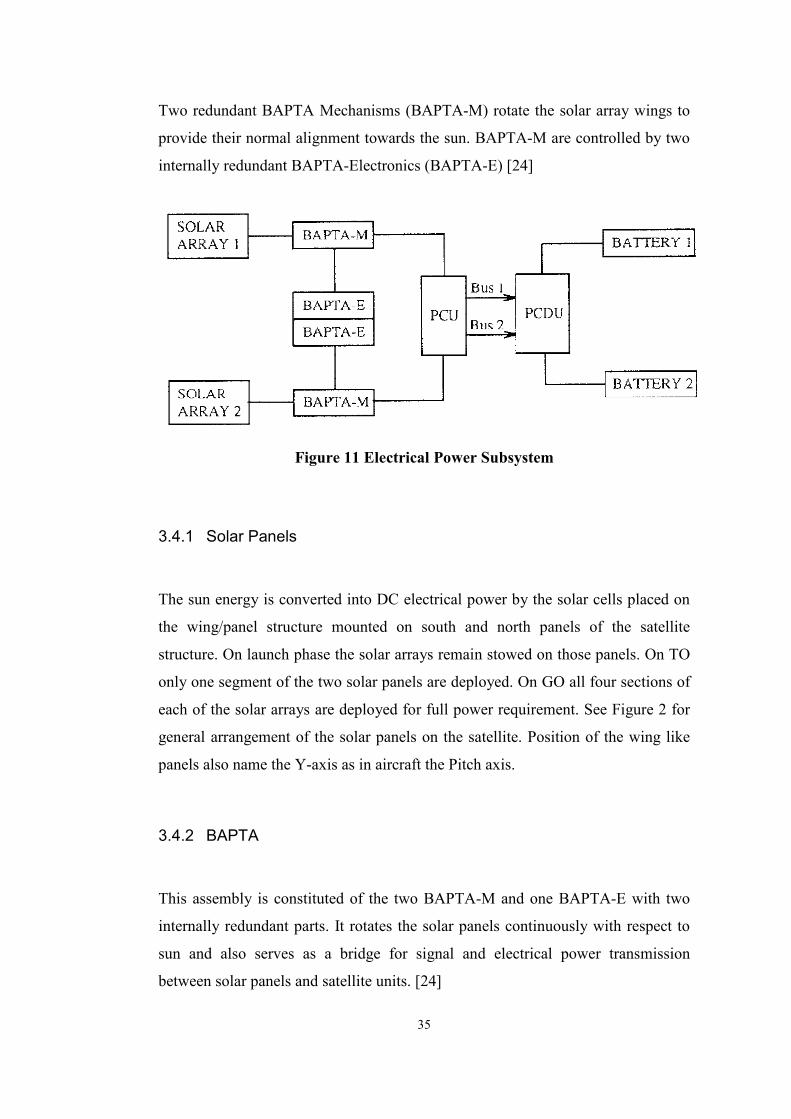
3.4 TÜRKSAT 1B Electrical Power Subsystem (EPS)
EPS provides electrical power to al the systems on the satellite (See Figure 11 [24]
for general arrangement) The electric source of the satellite is the solar panels.
They are always pointed normal to sunrays by the BAPTA –Bearing and Power
Transmission Assembly. Power Conditioning Unit (PCU) regulates the output
voltage obtained at solar panels. Again two redundant buses transmit the DC
electric power to Power Control and Distribution Unit (PCDU), where then the
electricity reaches to all required systems. Two sets of 27 celled Nickel / Hydrogen
batteries are the only electrical source when the satellite enters the moon’s or the
earth’s shadow (eclipse period), and prior to deployment of solar panels. They also
help to equalise the voltages on both busses. [24]
Page 42
35
Two redundant BAPTA Mechanisms (BAPTA-M) rotate the solar array wings to
provide their normal alignment towards the sun. BAPTA-M are controlled by two
internally redundant BAPTA-Electronics (BAPTA-E) [24]
Figure 11 Electrical Power Subsystem
3.4.1 Solar Panels
The sun energy is converted into DC electrical power by the solar cells placed on
the wing/panel structure mounted on south and north panels of the satellite
structure. On launch phase the solar arrays remain stowed on those panels. On TO
only one segment of the two solar panels are deployed. On GO all four sections of
each of the solar arrays are deployed for full power requirement. See Figure 2 for
general arrangement of the solar panels on the satellite. Position of the wing like
panels also name the Y-axis as in aircraft the Pitch axis.
3.4.2 BAPTA
This assembly is constituted of the two BAPTA-M and one BAPTA-E with two
internally redundant parts. It rotates the solar panels continuously with respect to
sun and also serves as a bridge for signal and electrical power transmission
between solar panels and satellite units. [24]
Page 43
36
BAPTA operates in three specific modes:
a) Cruise mode; one revolution per day in NM,
b) Acquisition mode; one revolution per 40 minutes,
c) Hold mode; panels fixed, no rotation.
3.4.3 PCU and PCDU
Each solar wing is composed of four panels of solar cells. Their total current
output is regulated by PCU. Shunting the current from all the sections to ground
with control of an error amplifier stabilizes the regulation of the voltage on two
buses. PCDU distributes the obtained electrical power to the satellite units.
Additionally it manages battery charging, controls temperature, and interfaces
telemetry between all the equipment of EPS and TCR Subsystem. See Figure 3 for
electric distribution for units of satellite systems. [24]
3.5 TÜRKSAT 1B Unified Propulsion Subsystem (UPS)
TÜRKSAT 1B benefits from the UPS based on reaction control logic. Except the
pitch control by FMW in NM all rotational (attitude) and translational (orbit)
maneuvers are actuated by the UPS. From TO- to drift orbit satellite is transferred
by means of three maneuvers actuated by 400 N apogee boost motors. From drift
orbit to GO 10N thrusters actuate N/S and W/S maneuvers. Orbit corrections are
ground commanded but attitude control is done automatically by onboard
algorithms of the ACDS. [24]
UPS is incorporated of the following units: [24]
a) One 400 N ABM motor
b) Twelve 10N thrusters
c) Two propellant tanks
d) One pressurant tank
Page 44
37
e) A set of valve control system
f) Two electronics units : UPSE (Also see Figure 3)
Total fuel and oxidiser has a mass of 942.8 kg, which is to be completely
consumed after de-orbiting. TÜRKSAT 1B uses monomethyl hydrazine, as fuel
and nitrogen tetroxide with 1% dissolved NO as oxidiser.
400 N ABM engine is used only for transmission from TO- to drift orbit, then
sealed and isolated from the UPS completely. Valve system of the boost motor and
the 10N thrusters also vary: 400 N motors use shut-off valves whereas 10N
thrusters use electrically powered on/off valves. UPSE serve as being an interface
between UPS and ADCS. [24]
3.6 TÜRKSAT 1B Telemetry, Commanding and Ranging (TCR)
Subsystem
This subsystem is mainly an interface between the satellite and the ground stations.
It performs three main functions: the telemetry, commanding and ranging to
control the operating mode which includes monitoring and command sending and
determination of the satellite orbit.
TCR subsystem equipment for on-station phase is: [24]
a) Communication antenna (also apart of the repeater subsystem)
b) Low noise amplifier (also apart of the repeater subsystem)
c) Couplers of telecommand signal for attenuation or amplification
d) Three receivers
e) Two transmitters
f) Two beacons
g) Switches for receive, transmit, beacon, and ranging redundancy
arrangements
h) Two authentication units.
Page 45
38
The receivers operate in hot redundancy, but transmitters and beacons operate in
cold redundancy. Hot redundancy means; in case of the nominal equipment fails,
the back up automatically switches on to continue the mission. On cold
redundancy ground commanding activates the back up equipment. [25]
3.7 TÜRKSAT 1B Repeater Subsystem
The main task of this subsystem is to receive the communication input signals that
are sent from earth, them to amplify them for transmitting back on the selected
coverage zones. In addition to this communication transmission task, the reception
of telecommand in GO, and telemetry transmission in TO and in emergency cases
are accomplished by this subsystem. [3]
3.8 TÜRKSAT 1B Thermal Control Subsystem
As its name implies its main task is to regulate, and maintain the temperature; or in
other words to provide a comfortable temperature environment within the satellite.
All the components, units in the satellite has its specific operational temperature
range, hence this subsystem keeps all the equipment within their reliable
operational temperature limits. Temperature regulation is achieved by two
functional types of elements: Active and Passive thermal controllers. [3]
Passive thermal control elements are; radiator panels with heat sinks or heat pipes,
optical solar reflectors, multilayer isolation blankets or foils, black or white paints,
interfillers, and shields.
Active elements are; the heaters, thermostats, and the thermistors. Class I heaters
are for temperature regulation of UPS components, sensors and batteries. Class II
heaters are for Repeater Subsystem. Thermostats are for IRES, RIGA, SSH
Page 46
39
heaters. Thermistors are the temperature sensors to initiate the routine or
emergency heater on/off switching.
3.9 TÜRKSAT 1B Mass Properties
Table 1 below summarises the mass property evolution during whole life of
TÜRKSAT 1B: [24]
Table 1
PHASE EVENT MASS (kg)
LAUNCH All appendages stowed 1783.678
B.O.T Solar array partially deployed
Reflector deployed 1783.678
E.O.T Solar array partially deployed
Reflector deployed 1082.578
B.O.L Solar array deployed Reflector Deployed
1082.578
E.O.L Solar array deployed Reflector Deployed
835.898
(Where BOT: Beginning of Transfer, EOL: End of Life, EOT, and BOL are as
similar.)
With the above mass change satellite also experience changes in moment of inertia
values and naturally satellite center of gravity (CG) is also altered during satellite
life. Maximum CG shift from BOT to EOL can be summarised in satellite
coordinates as: in x direction ∆X=79.51 mm, ∆Y=2.66 mm, ∆Z=1.38 mm. As
noticed total GC variation is very limited in Z and Y direction in comparison with
X direction. Similarly because of configuration and mass changes in TO, drift and
GO mass moment of inertia about the satellite principal axes are subject to large
changes. [24]
Page 47
40
Continuous regulation of the sun collector panels heading also has an effect on the
moment of inertia about the Roll (X) and Yaw (Z) axes. But keep in mind that the
panels are of thin light weight material and are not too long due to structural
(vibration, and so on) restrictions. Therefore cyclic change in the inertial values
will be very small. This attribute is sketched as Figure 12. This behaviour has
small impact on nominal thrust value of each thruster (impingement distortion).
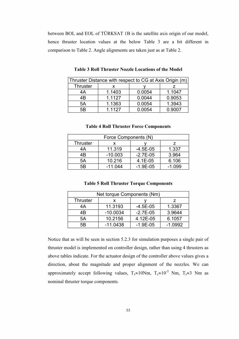
+ O
F
F
W
+ O
F
F
W
Same Force (F),same Weight (W)but differenttorques
Solar Panels
At timet1
At timet2
x or z
y
z or x
x or z
y
z or x
Figure 12 Reason how Ixx and Iyy change periodically
Page 48
41
CHAPTER IV
BUILDING OF A SATELLITE ATTITUDE DYNAMICS MODEL
SIMILAR TO THE TÜRKSAT 1B GEOSTATIONARY
SATELLITE
4.1 Introduction
Construction of a reliable attitude model for spacecraft is a vital step in
development of the automatic attitude control system. Careful building of the
motion equations is the first step of a simulation work. Simulations of a system
prior to functional component testing mock-up and/or prototype manufacturing
specifically for satellite production play very important roles. Simulation
capabilities are utilised for development time and cost reduction, validation and
verification, and also for reduction of training and maintenance costs.
Unlike aviation industry spacecraft industry, does not encounter mass production.
Hence an in-orbit prototype is not made, however an on-ground full-scale
engineering model for functional component and overall testing is manufactured.
The system designers and the manufacturer both appreciate the detection of design
errors early in design, and initialisation of the designed controllers’ optimisation.
Computer simulations also give a deeper insight into component functional tests
and the prototype or the manufactured item acceptance tests.
In this chapter, a mathematical model representing rigid body attitude dynamics of
a geostationary satellite platform similar to the TÜRKSAT 1B is derived for the
purposes of automatic control system design. First mass related properties are
Page 49
42
introduced, later equations of motion (EOM) using Newtonian mechanics with
definitions of reference coordinates and respective coordinate transformations are
derived, next actuator dynamics are also modelled, and finally environmental
disturbance torque are discussed to complete a full nonlinear attitude dynamics
model.
4.2 Mass Properties of the Model Spacecraft
4.2.1 General Description
TÜRKSAT 1B has a continuously decreasing mass behaviour, due to fuel
expenditure by thruster firings. Also inertial properties are affected from
deployment of solar panels. (Inertia values between Beginning of Transfer (BOT)
to End of Life (EOL) is variable due to mass loss) We will design our model with
mass properties similar to that of TÜRKSAT 1B. The control system we will
design concentrates on Geostationary Orbit (GO) attitude control. Therefore mass
and inertia values are selected with consideration of TÜRKSAT 1B BOL and EOL
properties. TÜRKSAT 1B experience about 250-kg mass reduction between BOL
and EOL. This results in a CG movement in XYZ directions of body coordinates
as: ∆X≈37mm, ∆Y≈1mm, and ∆Z≈1 mm.
The developed model assumes the Rigid Body representation of the satellite
structure is applicable. This representation neglects the effects of body elastic
modes. Rigid body model assumes the distance between any two points on the
satellite structure is constant.
Considering the CG movement of the TÜRKSAT 1B it is safe to assume that on
GO our model has a fixed CG location on the satellite structure. For a mass about
2000 kg CG movement of a few mm can be neglected for development of the
EOM and design of the controller. Hence attitude dynamics can be modelled as
rotational kinematics around the CG. Also this thesis we assume fixed moment of
Page 50
43
inertia values for design. Later it is possible to test the controller’s robustness to
changes in mass, CG locations and inertial parameters.
4.2.2 Determination of the Model Inertial Properties
In her thesis work Uslu [3] proposed the following inertia tensor:
2.
400000
06000
003600
mkg
IzzIyzIxz
IyzIyyIxy
IxzIxyIxx
I
=
−−
−−
−−
= (4.1)
It is noticed that she used principal axis frame where Product Mass Moment of
Inertia (PMMOI) values disappear. This is a valid approximation since TÜRKSAT
1B on its specific spacecraft coordinate frame PMMOI values are negligible in
comparison with Principal Moment of Inertia (PMOI) values. Uslu also proposed
PMOI values, which are also typical for geostationary satellites. Here our proposed
values are also close to those typical values, but also more specifically to
TÜRKSAT 1B to catch up its mass change effects. Again we will define the body
fixed reference frame also be principal. The following inertia tensor is used to
develop rigid body equations of motion:
2.
402000
07300
003770
mkg
IzzIyzIxz
IyzIyyIxy
IxzIxyIxx
I
=
−−
−−
−−
= (4.2)
4.3 Derivation of the Rigid Body Attitude Equations of Motion (EOM)
4.3.1 General Equations of Motion Description
Page 51
44
Newtonian mechanics is used to derive satellite rigid body EOM. In order to
derive EOM, an inertial reference frame is required, in which the Newtonian
mechanics is valid. The definition of an inertial frame states that the frame should
ideally be fixed, or be in uniform rectilinear translational motion relative to distant
stars. In this thesis “Earth fixed” reference frame can be taken as the inertial
reference, because our model satellite like TÜRKSAT 1B stay fixed on a specific
(42° East) longitude with zero inclination to earth equatorial plane in a circular
orbit with synchronous rotation with earth. (Always stays on same point as seen by
an earth observer.) Earth fixed coordinate system can be defined with the
following parameters: Its origin is the origin of spherical earth model with XE and
ZE on equatorial plane and YE pointing south. (See Figure 13)
To define the motion with respect to an observer on the satellite, the body fixed
reference frame, which is initially defined as a principal axes system, is used. The
body rates, moments, forces can easily defined in this frame. The origin of this
frame is the CG of the satellite. The x (roll) axis is aligned tangent to circular orbit
towards the satellite motion direction, y (pitch) axis is normal to the orbit plane
and directed towards south, z (yaw) axis is in the orbit plane and directed to earth
center.
Earth
x (roll)
y (pitch)
z (yaw)
Z
X
Y
E
E
E
Figure 13 Reference frame definitions
Where x, y, z represent the body fixed reference frame and XE, YE, ZE, earth fixed
reference frame.
NO
RT
H⇒
⇐
SO
UT
H
Page 52
45
Figure 13 [3] shows the orientation of the body fixed and the earth fixed reference
coordinate frames. Both these systems are defined as right-handed and orthogonal.
Earth fixed coordinate frame together with the satellite body-fixed frame rotates
with respect to an inertial frame at the orbit rate of one revolution per day
(ω0=7.272 10-5 rad/s)
The earth centered inertial reference frame is used for dynamic system of equation
derivation. As the set of states, the common practice is to choose angular velocity
components and attitude variables to define the 3-DOF (degrees of freedom)
rotational EOM. (The 3 translational components are not studied since this thesis
does not study orbital correction manoeuvres)
4.3.2 Model’s EOM Description
The angular momentum of a rigid body around its center of mass (here CG is
assumed to coincide with center of mass) determined by the following relation:
∫ ××= dmrrH )( ω (4.3)
Where the integration is done over the whole mass body as represented in a
generic way by Figure 14. In this generic formula r (or equivalent representation
by “r” denotes the location vector of a particle inside the body, and ω (or
equivalent representation by ωωωω) is the angular velocity vector of the body defined
by “B”.
Page 53
46
BR0
CG
dm
r
x
y
z
Figure 14 Generic sketch for EOM derivation
Evaluating the above vectorial integral and decomposing, we obtain the angular
momentum of the body B. Here ωx,y,z are the body angular rates.
hx= Ix ωx- Ixy ωy -Ixz ωz (4.4.a)
hy= -Ixy ωx +Iy ωy -Iyz ωz (4.4.b)
hz= -Ixz ωx -Iyz ωy +Iz ωz (4.4.c)
Inertia tensor is very simplified by use of the principal axes. PMMOI components
of the inertia matrix vanished, hence the angular momentum vector simplifies to:
hx= 3770 ωx (4.5.a)
hy=730 ωy (4.5.b)
hz= 4020 ωz (4.5.c)
The total applied torque (T) on the system about its center of mass is equal to the
time rate change of the angular momentum.
T=dH/dt (4.6)
or
Page 54
47
HωH
T ×+
=bodydt
d (4.7)
where bodydt
d
Hdefines the derivative in body axis frame.
Without adding the momentum wheel effect the Euler equations yield:
zyyzxxx ωω)I(IωIT −+= ɺ (4.8.a)
zxzxyyy ωω)I(IωIT −+= ɺ (4.8.b)
yxxyzzz ωω)I(IωIT −+= ɺ (4.8.c)
with the addition of inertia values the torque equation becomes:
zyxx ωω3290ω7703T += ɺ (4.9.a)
zxyy ωω250ω730T −= ɺ (4.9.b)
yxzz ωω3040ω0204T −= ɺ (4.9.c)
At the above derivation there exists no explicit disturbance effect. The thruster
control torque values shall appear on the left side inside Tx,y,z torque components.
(Momentum wheel effect is separately discussed in the following section. Right
hand side of the equations represents undisturbed free body motion in principal
axis frame.
We reference the satellite attitude to earth fixed reference frame hence to obtain
angle data from angular velocity in body fixed frames we need a conversion
method to integrate the velocity vector correctly.
For small angular variations Euler angle transformation is easily implemented, and
also it is easy to understand from its construction geometry.
Page 55
48
4.3.2.1 Euler Angle Transformation
Euler angle transformation gives the attitude of the spacecraft with respect to an
Earth-Fixed observer. Starting from earth’s axes, with three rotations in a specific
order, it is possible to obtain attitude representation of the satellite in body-fixed
axes. These angles are defined as follows:
φ → Roll angle about (x) axis
θ →Pitch angle about (y) axis
ψ →Yaw angle about (z) axis
The transformation is not a commutative operation hence the order of the
transformation is important. Different sequences yield different resultant matrices.
For our model we select the rotation sequence about the angles: yaw (ψ), roll (φ)
and finally pitch (θ).
We define the body fixed principal (xyz) coordinate system with ebody vector and
an orbital frame fixed on the satellite (XYZ) orbit as the Eorbit. (See Figure 15. [26])
Page 56
49
Figure 15 Geometry for orbital axis definition
orbitalbodyE
E
E
e
e
e
=
3
2
1
3
2
1
θφψ RRR (4.10)
Rotation sequence can be visualized as below Figures 16 and 17:
Eorbit Em En ebody
uk(orbit) ui
(m) uj(n)
ψ φ θ
R3(ψ)=eUiψ R1(φ)=eUjφ R2(n,b)=eUkθ
Figure 16 Transformation sequence
Page 57
50
φ
φ
ymxm=xn
yn
zn
zm
Xψ
ψ
Xorbit
Yorbit
Zorbit=zm
xm
ym
θ
θ
xnyb=yn
xb
zb
zn
Figure 17 ψψψψ-φφφφ-θθθθ Rotation sequence from orbit fixed to body fixed frame
There we obtain the following rotation matrices:
−
=
100
0
0
) ψψ
ψψ
ψ cs
sc
(R 3 ,
−=
φφφφφ
cs
sc
0
0
001
)(R1 , and
−
=
θθ
θθ
θcs
sc
0
010
0
)(R 2
(4.11 a, b, c)
Where the s( ) and c( ) define the sine and cosine functions respectively.
The individual rotations can be expressed as:
morbitz
y
x
Z
Y
X
=
)(ψ3R ,
nmz
y
x
z
y
x
=
)(φ1R , and
bnz
y
x
z
y
x
=
)(θ2R (4.12)
The angular velocity components ω1, ω2, ω3 in the spacecraft principal body fixed
reference frame are given by,
+
+
+
=
0
ω
0
)()()(
0
0
)()(
0
0)(0
0
0
3
2
1
θφψθφψφ
ψψω
ωω
213133 RRRRRR ɺ
ɺ
ɺ
(4.13)
Where ω0 is the earth rotation rate of 7.272 10-5 rad/sec. And performing the
respective matrix multiplication the body rates yield the following result,
Page 58
51
+−
++−
++
=
=
)sin()ω(
)cos()cos()ω()sin(
)cos()sin()ω()cos(
0
0
0
3
2
1
φθψφψθψφφψθψφ
ωωω
ωωω
ɺɺ
ɺɺ
ɺɺ
z
y
x
body
(4.14)
Defining 10 )ω( θθ ɺɺ =+ we can take the inverse left part of the above equation to
get,
++
+
−
=
zyx
yx
yx
ωφψωφψωφψ
ωφψ
ω
ψωψω
ψθφ
)tan()cos()tan()sin()cos(
)cos(
)cos(
)sin()sin()cos(
1
ɺ
ɺ
ɺ
(4.15)
replacing θθ ɺɺ =− )ω( 01
++
−+
−
=
zyx
yx
yx
ωφψωφψωφψ
ωφψ
ω
ψωψω
ψθφ
)tan()cos()tan()sin(
ω)cos(
)cos(
)cos(
)sin()sin()cos(
0
ɺ
ɺ
ɺ
(4.16)
This is the final equation representing Euler rates in body coordinates. As noticed
from the above set of equations the system is singular at 90° roll angle (φ=90°),
since 1/cos(90°) is infinity. For different selections of the rotation sequences any
of the rotation angles may experience this singularity. Above set is selected to
avoid a singularity at pitch angle specifically. Having limitations on these angles
does not interrupt us, because satellite is to offset maximum ±6° as previously
noted on section 3.3.7 and on NM pitch and roll attitudes are maintained within
±0.05° bias. [3] As a result satellite is not expected to experience high changes in
roll/pitch attitude during service orbit life.
Another way of representing the attitude information is the "quaternion" technique.
Quaternion representation has the advantage of not having the singularity in
Page 59
52
coordinate transformations. Also it increases the on-board computation speed
which is critical for navigation, strapdown systems. Unfortunately with this
method, it is hard to visualise the actual angles. In this thesis there is no need to
use the quaternions. Euler representation is reliable, simple and accurate enough.
4.3.2.2 Including the Momentum Wheel Torque to Euler Equations
The previously derived
zyxx ωω3290ω7703T += ɺ (4.9.a -repeated)
zxyy ωω250ω730T −= ɺ (4.9.b -repeated)
yxzz ωω3040ω0204T −= ɺ (4.9.c -repeated)
equations excluded the momentum wheel torque. Similar to TÜRKSAT 1B
arrangement we select a momentum wheel whose total torque is aligned with –y-
axis (negative pitch axis) of the satellite. In vectorial representation the angular
momentum equation is modified as follows in Cartesian representation (i,j,k
representing unit vectors along the x,y,z directions):
kjiH zzwyyxx III ωωω +−+= )h( (4.17)
Where hw represents the nominal torque of the momentum wheel. (hw=60 N.m just
as Reference [3] proposed) Then with the application of Euler angular momentum
law (Equation 4.7) we get the following result:
zzyxx ω60ωω3290ω7703T ++= ɺ (4.18.a)
whωω250ω730T zxyyɺɺ −−= (4.18.b)
xyxzz ω60ωω3040ω0204T −−= ɺ (4.18.c)
Page 60
53
Here whɺ represent the time rate of change of wheel angular momentum, which
defines the pitch control law. In case no pitch control is applied it vanishes
( 0h =wɺ ).
4.3.2.3 Thruster Geometry and Torque Definitions
Similar to TÜRKSAT 1B our model also uses the offset oriented thrusters to get
coupling for passive yaw control. The generic orientation can be visualized by the
following Figure 18:
FX(S/C)
FY(S/C)
FZ(S/C)
X(S/C)
αβ
Y(S/C)
Z(S/C)
Fthruster
F.cosββββ
Figure 18 Generic thruster orientation angles
Where the (S/C) denote the spacecraft coordinate frame. We can easily conclude
from the above Figure that the X(S/C), Y(S/C), Z(S/C) components of the force vector
Fthruster are:
Fthruster=F (10N nominal) (4.19.a)
FX(S/C)=F.cosβ.cosα (4.19.b)
FY(S/C)=F.cosβ.sinα (4.19.c)
FZ(S/C)=F.sinβ (4.19.d)
Page 61
54
We computed the exact torque components of the TÜRKSAT 1B with the
inclusion of impingement forces. The value arising from the impingement
characteristics were negligible (less than 1% of maximum component) Also
Reference [3] notes this feature, hence in this thesis we also exclude impingement
characteristics.
This thesis will use canted roll thrusters with similar location and alignment to that
of TÜRKSAT 1B. The control system will be designed in accordance with use of
only roll thrusters, which is the nominal case in NM during GO.
Nominal thrust magnitude is 10 N. Thruster 4A, 4B, 5A, 5B of TÜRKSAT 1B are
used. On/off valves similar to TÜRKSAT 1B control the attitude thrusters of our
model. .
In TÜRKSAT 1B the orientations of the south thrusters are as at Table 2:
Table 2 TÜRKSAT 1B Roll Thruster Properties
Locations Thruster Orientation Thruster
X (mm) Y (mm) Z (mm) α (deg) β (deg) 4A 2200 0 -1100 0 -16 4B 0 0 900 180 7 5A 2200 0 1380 0 26 5B 0 0 -900 180 -7
However with above location coordinated CG is not at the origin. A Microsoft
Excel worksheet calculates the net torque over our model of satellite with the CG
at the origin of satellite body fixed coordinates. (Tables 3-5) In TÜRKSAT 1B CG
change during BOT to EOL also changes the moment arms of the thrusters, which
causes alterations on the effective torque values of the thrusters. However since
our model assumes a fixed CG location, moment arm length is fixed for our study
during NM at GO (BOL to EOL). Our model has the below thruster characteristics
where moment arms (the location of thruster's nozzles with respect to the satellite
CG) are approximately nominal to that of TÜRKSAT 1B. The average CG
Page 62
55
between BOL and EOL of TÜRKSAT 1B is the satellite axis origin of our model,
hence thruster location values at the below Table 3 are a bit different in
comparison to Table 2. Angle alignments are taken just as at Table 2.
Table 3 Roll Thruster Nozzle Locations of the Model
Thruster Distance with respect to CG at Axis Origin (m) Thruster x y z
4A 1.1403 0.0054 1.1047 4B 1.1127 0.0044 0.9053 5A 1.1363 0.0054 1.3943 5B 1.1127 0.0054 0.9007
Table 4 Roll Thruster Force Components
Force Components (N) Thruster x y z
4A 11.319 -4.5E-05 1.337 4B -10.003 -2.7E-05 3.964 5A 10.216 4.1E-05 6.106 5B -11.044 -1.9E-05 -1.099
Table 5 Roll Thruster Torque Components
Net torque Components (Nm) Thruster x y z
4A 11.3193 -4.5E-05 1.3367 4B -10.0034 -2.7E-05 3.9644 5A 10.2156 4.12E-05 6.1057 5B -11.0438 -1.9E-05 -1.0992
Notice that as will be seen in section 5.2.3 for simulation purposes a single pair of
thruster model is implemented on controller design, rather than using 4 thrusters as
above tables indicate. For the actuator design of the controller above values gives a
direction, about the magnitude and proper alignment of the nozzles. We can
approximately accept following values, Tx≈10Nm, Ty≈10-5 Nm, Tz≈3 Nm as
nominal thruster torque components.
Page 63
56
4.3.2.4 MATLAB-Simulink Uncontrolled Behaviour Graphical Results
This uncontrolled attitude dynamics simulation study is represented at APPENDIX
A where we also included the discussion of the results by comparisons. Next step
is to explain environmental (external) and internal disturbance effects on the
satellite dynamics.
4.4 Environmental and Internal Disturbances on Attitude Model
The primary environmental disturbing effects concerning the spacecraft attitude
are the solar radiation pressure, gravity gradients, aerodynamic and magnetic
disturbing torques on satellite body. These are the external disturbances, and the
other group of perturbations is the internal ones; which primarily includes the
effects associated with internal moving hardware, thrust misalignment, propellant
leakage or slosh effects, and so on.
From the environmental perturbation group, the solar radiation pressure is
significant on both attitude and trajectory biases of the satellite for altitudes higher
than 1000 km. The gravity gradient disturbance torques, result from the extended
dimensions of the geostationary satellite. The magnetic perturbations arise by
interaction of the satellite magnetic materials with earth's magnetic field and are
most significant below 1000 km. Similarly Aerodynamic perturbations are most
significant below 500 km and are negligible over 1000-km altitudes. These effects
are visualised by the Figure 19. ( [26] and [30] )
As for the other group, the internal perturbation torques group, the torques arising
from internal moving parts have several causes such as, rotating wheels, scanning
devices, circulating fluids, and so on. These effects must be included in the general
equations of motion of the satellite attitude. Propellant slosh, leakage, and
misalignment of the momentum exchange actuators (thrusters, momentum wheels
and so on) cause deviation on satellite kinetic energy and momentum distribution
among components affecting its attitude. [26]
Page 64
57
Figure 19 Typical perturbation torques as a function of altitude
4.4.1 Environmental (External) Disturbance Torques
Here we present the mathematical models for environmental disturbing torques on
satellite attitude. On the simulation model only solar radiation and gravity gradient
torques have significant effects because TÜRKSAT 1B has a high altitude of
36000 km on its geostationary orbit. Also refer to Figure 19.
4.4.1.1 Solar Radiation Pressure Torque
The photons from the sun produce a net torque with their impingement on the
various distinct surfaces of the satellite structure. According to the satellite attitude
with respect to sun and its geometrical shape the incident photons produce net
force components on each distinctive satellite segment. The total net perturbing
torque is a result of these components, which are biased with satellite center of
mass. This disturbance torque mainly depends on the following factors: [26] and
[2]
Page 65
58
a) Satellite Geometric Configuration. This configuration influences the
degree of shading and the net moment arm of the net force with respect
to satellite mass center.
b) Shading Effects. Some components of the satellite structure surely will
not be exposed to sunrays due to the other component's shades over
them. Satellites with large protruding parts experience significant
effects of shading.
c) Optical Reflection Properties of the Satellite Surface.
d) Satellite-Sun Vector Orientation. The time history of the satellite, the
orbital position and inclination with respect to sun, affects the shading
and the total amount of solar radiation absorbed/reflected.
The solar radiation torque on a satellite is in the form: (Chobotov [26])
∫= se
solar fdxrT.
)(
(4.20)
Where r
is the vector directed from the satellite center of mass to the area element
dAi for the i-th surface, and e.s represents the sun exposed surface
The latter differential force vector may be modelled assuming that the incident
radiation of the sun is either reflected (specularly or diffusively) or absorbed, or
some combination of these. The following formula is given [3].
dANCCSCPfd dsatotal )cos()3
1)cos((2)1( θθ∫
++−−=
(4.21)
Here coefficients Ca, Cs, Cd define the percentage of the absorbed, specularly
reflected and diffusively reflected radiation, respectively. P is the mean
momentum flux, S
is the unit vector from the satellite to the sun, N
is the unit
vector along the normal of the exposed surface, and θ is the angle between S
and
N
. The integral is taken over the surface area (dA: infinitesimal area element).
Page 66
59
However it's very difficult to apply these relations to our case of Geostationary
Satellite.
Figure 20 Reflection types [26]
Chobotov also proposes the following general formula for a geosynchronous
satellite for a given season [26]. The fundamental Fourier components of solar
torque about the body axes are:
T1(s)= A + B cos(ω0t) + G sin(ω0t) (4.21 a)
T2(s)= E + F cos(ω0t) + I sin(ω0t) (4.21 b)
T3(s)= C + D sin(ω0t) + H cos(ω0t) (4.21 c)
where A to H are constants.
Kaplan ([27]) proposes a more explicit model. A cyclic model for a three-axis
stabilised satellite configuration. The model resembles to the above set of
equations proposed by Chobotov.
Tx=2 10-5 [1-2 sin(ω0t)] (4.22 a)
Tx=10-4 cos(ω0t) (4.22 b)
Tx=-5 10-5 cos(ω0t) (4.22 c)
Page 67
60
This model is used for this thesis, at the Matlab-Simulink simulation model. The
above set of equations are transferred into Matlab-Simulink as follows:
Figure 21 Solar pressure disturbance, simulink implementation
The time history of the perturbation torque is:
Figure 22 Solar radiation pressure time history (torque in Nm)
Page 68
61
4.4.1.2 Gravity Gradient Torque
This perturbation torque occurs because of the small difference in the strength of
the earth gravitational field over the satellite structure.
Hughes [28] proposed the following mathematical relation, the gravity gradient
torque acts on a general body with principal moments of inertia I1, I2, I3 as:
g = −3(GM / R3)[(I2-I3) θ1, (I1-I3) θ2, 0] (4.23)
where θ1, θ2, θ3, represent the small rotation angles about the principal axes. For
circular (as in the case of geostationary) orbit GM/R3 is equal to the square of
orbital angular velocity, ω0. R is the distance between the earth and the satellite
mass center.
Chobotov proposes a more complex model with principal body axes; the gravity
gradient torque in component form is as follows:
T1(g) = K (I33-I22) a21 a31 (4.24 a)
T2(g) = K (I11-I33) a11 a31 (4.24 b)
T3(g) = K (I22-I11) a11 a21 (4.24 c)
where K=3µ/R3 and aij (i, j=1,2,3) are the elements of the transformation matrix
(i.e., direction cosines). (µ=GM the earth gravitational constant). This equation
also simplifies to equation set 4.26 with proper assumptions.
The location of the satellite center of gravity (CG) changes according to its
attitude, which is the angular arrangement with respect to gradient of the potential
field and the distance between the satellite and the attraction center (the earth).
[29] This yields a net torque in addition to the attraction force, and is called gravity
gradient torque.
Page 69
62
Rimrott proposes a very similar form of equations like Chobotov. With the small
satellite assumption the torque of the Kepler force about the satellite's mass center
the following set of equations result:
[ ]
−
−
−
Ω=
)cos()cos()(
)cos()cos()(
)cos()cos()(
3 2
βααγ
βγ
AB
CA
BC
eee zyxM (4.25)
where α, β, γ are the direction angles between the position vector ρρρρ and the
satellite principal axes. A, B, C are the components of the inertia tensor along the
principal axes. Ω2=µ/ρ3C and ρC is the distance between satellite mass center and
the earth center. Note that small satellite approximation yields the following
approximation: µ/ρC ρ2G ≈µ/ρ3
C =Ω2. When position vector and the principal axis
directions coincide, this equation takes the simple form of the model proposed by
Kaplan [27], which we are to present next:
Kaplan [27] simplifies the above stated general formulas to yield following set of
linearised equations in component form:
Tx(g)=-3ω0
2(Iy-Iz) φ (4.26 a)
Ty(g)=-3ω0
2(Ix-Iz) θ (4.26 b)
Tx(g)=0 (4.26 c)
Kaplan derives this set of equations using the simple form of the motion equation,
dt
dhG = where G is the gravity gradient net torque vector, and h is the net angular
momentum vector of the rigid satellite.
Finally Bryson [30] proposes the above relation with minor symbology difference:
[ ]kIIjIIiIIR
gQ yxxzyzg
ˆ)(ˆ)(ˆ)(3 φθθφ −+−+−=
(4.27)
Page 70
63
where he also states that the multiplication φθ is negligible and 3g/R≈ω20.
As Uslu [3] Kaplan and the others we are going to use this model (4.26) of gravity
gradient disturbance torque for the simulations by Matlab-Simulink. Inserting the
model inertia values we finally obtain the following set of equations for gravity
gradient perturbing torque:
=
−
−
0
1096637.3
1021975.56
5
θφ
z
y
x
G
G
G
(4.28)
4.4.1.3 Aerodynamic and Magnetic Disturbance Torques
• Aerodynamic Torque
This perturbation force is most dominant for low altitude satellites orbiting below
approximately 400-500 km. The drag force components created by the air
molecule interaction with the satellite body produce a net torque about the satellite
center of mass. The satellite passes through an atmosphere of density ρ with a
velocity vector v. The magnitude of the aerodynamic drag force F(a) is then given
as:
F(a) = ½ ρ v . v ACd (4.29)
where A is the reference area of the satellite (i.e., cross-section along v) and Cd is
the drag coefficient. Then the total torque is given by:
T(a)=½ ρ v2 l S Cd (4.30)
Page 71
64
where l is the length of the perpendicular from the mass center to the force line of
action. Chobotov offers some estimates on Cd and air densities.
Uslu [3] offers the same formula in differential form. Uslu and Hughes and
Chobotov emphasis that the aerodynamic torque becomes comparable with the
gravity gradient perturbation on low altitudes between 100-600 km. For
TÜRKSAT 1B geostationary satellite which is at high altitude (~36000 km) this
perturbing torque can safely be neglected. Refer to Figure 19 as well.
• Magnetic Disturbance Torque
Magnetic disturbance torques on a satellite result from the interaction of the
spacecraft's residual magnetic field and geomagnetic field. Let M be the sum of all
magnetic moments in the satellite the torque acting on it is: ([3] and [26])
T(m)=MxB (4.31)
where B is the geomagnetic field vector (also named as geocentric magnetic flux
density). Generally M is caused by permanent and induced magnets or by satellite
generated current loops.
As emphasised by Uslu and Chobotov this perturbation is also negligible for a
geostationary satellite at high orbit. Refer to Figure 19 as well.
4.4.2 Internal Disturbance Torques
The internal torques that we will shortly describe here show completely random
behaviour. Therefore we are unable to propose explicit mathematical models as in
the case of environmental effects. Also their perturbing magnitudes are small in
comparison to external torques hence they are neglected for the simulations.
Page 72
65
4.4.2.1 Mass Expulsion Torque
They are the results of the propellant or other mass ejection from the satellite.
They can be investigated in two groups according to their sources: [3]
a) Unintentional control system torques. These include the fuel leakage,
thrust vector misalignment, anomaly in the thruster firing time, reaction
forces due to plume impingement.
b) Torques due to sources intended to expel mass. These include dumping
residual propellant, payload separation, payload ejection, equipment
jettison, and orbital manoeuvre's impact.
One note on plume impingement is that for TÜRKSAT 1B the measured
maximum plume impingement of the roll thrusters is about 1% of the nominal
control torque which is also neglected when we represented the model satellite's
actuator properties. (Section 4.3.2.3)
4.4.2.2 Propellant Slosh Torque
The rotational or the translational accelerations of the satellite causes sloshing of
the fluids inside the satellite which is generally only the propellant in partially
filled fuel tank and pipes. The duration and magnitude of the sloshing depends on
the propellant properties, tank/pipe geometry, the amount of fluid in the
tank/pipes, and the acceleration field [2] , [3].
4.4.2.3 Moving Hardware Torques
Motions of some satellite components like antennas, solar array wings, hardisk of
the microcomputers also produce disturbance torques.
Page 73
66
CHAPTER V
ATTITUDE CONTROL SYSTEM DESIGN
5.1 Pitch Control System Design
Initially the pitch motion is decoupled from the yaw/roll dynamics, then the
equations are converted into state space representation.
5.1.1 Equations for Pitch Motion
At Appendix 2 the nonlinear governing motion equations are linearised. The
decoupled pitch attitude equation is :
hθ730θ103.8722T 7y
ɺ+=+ −..
(5.1)
where Ty is only the solar pressure perturbation torque, and hɺ is the momentum
wheel control law – basically the momentum wheel acceleration/deceleration
value. Without the control hɺ , pitch motion is unstable. The gravity gradient
perturbing torque shifts the body dynamics system from double poles at origin to,
one positive one negative real pole close to origin. (See the eigenvalues calculation
in Appendix 2.) The pitch motion equation is converted into state space
formulation for better representation in Simulink program. Setting the states X1=θ
and X2=dθ/dt, we get the state equation in form uBXAX +=ɺ and the output
equation in form XC=y . Where the system representing matrices are as follows:
Page 74
67
= − 0103043.5
1010
A is named as system matrix, and its eigenvalues
determine the stability characteristics.
= −310369863.1
0B is the input matrix.
The outputs of the system are the states, hence the respective measurement matrix
C is a 2x2 unity matrix,
=
10
01C .
Finally u is the control law hɺ , which is determined by the following sections.
One remark may be that the rate information (dθ/dt) is assumed to be measured by
rate gyros and the attitude (θ) information is measured by optical earth/sun
sensors. Here our model differs from the original TÜRKSAT 1B control
configuration. We propose a controller that needs measurement of both rate and
attitude information for precise attitude regulation whereas original TÜRKSAT 1B
controller needs measurement of attitude only.
5.1.2 Actuator Model
Second order DC motor representation is selected for accurate torque control. Both
Ogata [31] and Kuo [32] uses this second order model throughout their control
books for position control purposes. The model is modified for torque control to
get the angular moment output rather than angular position output. The block
diagram is given in Figure 27. The physical parameters of the DC motor for
TÜRKSAT 1B was not available hence in this thesis an actuator model is
assumed. Various stabilizing parameters are determined by rootlocus analysis
however many of them require very high gains for the PD controller hence one of
Page 75
68
most feasible configuration is represented here. The 'load actuator' block in the
main program for control of linearised pitch dynamics is used to test various DC
models for transient responses. It is a simple Matlab m file that loads motor
parameters into Matlab Workspace when clicked on the respective block in main
Simulink program.
Physical parameters of designed actuator are:
La=0.005(H) Armature inductance,
Ki=0.3 (N-m/A) Torque constant,
Kb=0.3 (V/rad/s) Back EMF constant,
Bm=0.002 viscous-friction coefficient;
Jw=0.12456 (kg m2) total (rotor+wheel) inertia of motor,
Ra=5 (Ω) Armature resistance
The following transfer function represents the DC motor model. It has the system
poles at –999.86 and –0.16059, and the system zero is at –1.6057 10-2 locations.
5652.160s016.1000s
96339.0s602 ++
+ (5.2)
The satellite dynamics is represented by the transfer function (5.3). The system has
one stable pole at –2.3031 10-5 and one unstable pole at 2.3031 10-5 .
102
3
103044.5s
103699.1−
−
− (5.3)
Finally the transfer function for the PD controller is (Kd s + Kp ), which
introduces a zero to the closed loop system at –Kp/Kd.
The following m file is written to obtain the rootlocus plot of the actuator, satellite,
PD Controller blocks together;
Page 76
69
KpKd3=-20;
Z3=[-1.6057e-2 KpKd3];
P3=[-2.3031e-5 2.3031e-5 -999.86 -1.6057e-1];
SYS3=ZPK(Z3,P3,1);
rlocus(SYS3)
title('R=5, L=0.005, B=2e-3, K=0.3')
Figure 23 Rootlocus diagram for controlled pitch attitude
Below set of figures show various zoomed sections of above Figure 23. Each
zoomed section present the regions about system poles (defined by an X mark) and
system zeros (defined by an O mark).
Page 77
70
Figure 24 Zoomed sections of Figure 23
Actuator poles are at, s1=–999.86 and s2=–0.16059 and the zero is at z=–1.6057
10-2. The actuator itself is stable with relatively fast dynamics in comparison with
satellite attitude dynamics whose unstable poles are placed at s1,2=±2.3031 10-5.
Figures 23 and 24 are the overall closed loop rootlocus diagrams with PD
controller zero at –20 (-Kp/Kd zero location for controller, Kp=50, Kd=2.5 is found
appropriate after several trials on Simulink model).
5.1.3 PD Controller Design: Tuning the Parameters
From the Rootlocus analysis the most appropriate location for the zero defined by
the PD controller (Kp + Kd . s) is between the actuator most right pole and the
most left pole This configuration gives a stable pitch behaviour.
Also with the help of NCD (Nonlinear Control Design) optimisation built-in-block
of Simulink, a neutrally stable configuration can be obtained. This design is later
refined by tuning the gains of the PD controller. After several such trial and error
study, Kp≥50 and Kd≈2.5 is found satisfactory to keep the satellite's maximum
controlled pitch attitude for expected disturbances between 0.8336±0.05 °. Lesser
Kp values result in single overshoot at initial seconds to initial position errors,
whereas higher Kd requires higher Kp which both multiplies the measurement
Page 78
71
errors. Also higher Kd may result in several oscillations before settling around the
nominal angle.
Solar radiation pressure disturbance is also successfully suppressed by the above
selection of Kp, and Kd control variables. The control system short term response
to both positive and negative biases around nominal settling angle and long term
response to solar radiation are represented through Figures 31-35.
Measurement process is assumed to be noisy hence 'Band Limited White Noise'
blocks are added to system outputs (Roll angle and rate). The magnitude of the
measurement error is assumed to be on the order of maximum (±0.00005° and
±0.00001 °/s).
As a result PD controller with (Kp=50, Kd=2.5) gains can damp ±0.1° bias from
nominal without any overshoot and dangerous oscillations. Also this selection is
satisfactory to suppress solar radiation cyclic disturbances and can reject the
random measurement errors of about (±0.00005° and ±0.00001 °/s). These gains
are also experimented with the final nonlinear model and are found satisfactory.
5.1.4 Simulink Program for the Simulation of the Linear Pitch Dynamics
Model, together with the Controller
Page 79
72
Figure 25 The main Simulink model for control of linearised pitch dynamics
The yellow blocks are the sub-systems represented at Figures 26-30.
Figure 26 Linearised state space representation of pitch dynamics
Figure 27 PD controller
Page 80
73
Figure 28 Second order DC motor (actuator) model
Figure 29 Solar radiation pressure disturbance model
Figure 30 Data storage and displays model
5.1.5 Linear Simulation Results
Figures 31-35 show time histories of the controller's response to two different
initial attitude bias angles and to external disturbance torque of solar pressure
radiation and gravity gradient. Two cases for initial attitude bias are defined as
follows:
CASE 1 θ0=0.8336-0.1° and CASE 2 θ0=0.8336+0.1°. Figures 31 and 33 are
simulations for CASE 1, Figures 34, 35 are for CASE 2.
Page 81
74
0.71
0.73
0.75
0.77
0.79
0.81
0.83
0.85
0.87
0.89
0 20000 40000 60000 80000 100000
Time (s)
Pit
ch
An
gle
(d
eg
)
Figure 31 Pitch attitude long-term
response for CASE 1
0.72
0.74
0.76
0.78
0.8
0.82
0.84
0.86
0.88
0.9
0 500 1000 1500
Time (sec)
Pit
ch
An
gle
(d
eg
)
Figure 32 Pitch attitude zoomed (0-
1500 sec) response for CASE 1
-0.001
-0.0005
0
0.0005
0.001
0.0015
0.002
0.0025
0.003
0 500 1000 1500
Time(sec)
Pit
ch
Ra
te (
de
g/s
)
Figure 33 Pitch rate zoomed (0-1500 sec) response for CASE 1
0.76
0.78
0.8
0.82
0.84
0.86
0.88
0.9
0.92
0.94
0 20000 40000 60000 80000 100000
Time (s)
Pit
ch
An
gle
(d
eg
)
Figure 34 Pitch attitude long-term
response for CASE 2
0.72
0.77
0.82
0.87
0.92
0.97
0 500 1000 1500
Time (sec)
Pit
ch
An
gle
(d
eg
)
Figure 35 Pitch attitude zoomed (0-
1500 sec) response for CASE 2
Page 82
75
The selected gains (Kp=50, Kd=2.5) for the pitch controller can suppress both long-
term solar radiation disturbance and short term initial attitude bias successfully.
Also below Figure 36 shows that the actuator is not saturated with this selection of
control gains. The produced torque is not very high to saturate the actuator.
Zoomed for first 100 seconds
Simulation for 1000 seconds
Figure 36 Pitch actuator output torque
5.2 Roll/Yaw Control System Design
The Roll/Yaw coupled equations of motion are linearised in Appendix B. The
eigenvalues analysis in Appendix B shows that, the uncontrolled system is
marginally stable with relatively low frequencies. (Both the roll and yaw have
imaginary poles with no real parts). Since the actuators are the thrusters, they shall
be modelled as nonlinear on-off type modulators for Simulink model. This
introduces nonlinearity to the simulation, which requires careful design. After
presenting the respective motion equations required for satellite body dynamic
model, control law development, and actuator implementation are discussed.
Finally the control parameter tuning for best control with fuel minimisation in
mind, is presented.
Page 83
76
5.2.1 Linearised Equations Of Roll/Yaw Coupled Motion
Equation (5.4) represents the roll/yaw coupled linear attitude dynamics.
−
−+
−
+
=
−
−
ψφ
ψφ
ψ
φ3
3
1036.10
01037.1
00091.60
1604.600
40200
037700
ɺ
ɺ
..
..
(5.4)
This equation can be put into state space formulation, which is used in Simulink
model more conveniently. uBXAX +=ɺ and the output equation in form
uy DXC += .
This time since the motion is coupled, matrix dimensions are increased. The states
are defined as ψX,Xψ,X,X 4321ɺɺ ==== φφ . Then the respective A, B, C,
D matrices are as follows:
−=
−−
−−
01049276.1103911.30
10595767.100106342.3
1000
0100
27
27A (5.5)
=
−
−
4
4
104876.23.0
106525.2
0
0
x
B (5.6)
Here we again aim to design a controller which needs all the states' information,
hence the output relation becomes, C=4x4 unity matrix and D=[0 0 0 0].
The B matrix is 1x4 vector. We selected the thruster similar of TÜRKSAT 1B
which also have "canted" set of roll/yaw thrusters. That is 'roll' thruster firing also
accompanied by a yaw torque due to the alignment of the thruster with respect to
Page 84
77
satellite frames. The degree of thruster coupling is selected to be 0.3 after several
controller designs for various thrust coupling levels. Thus, 1Nm torque in the roll
axis causes 0.3 Nm torque in the yaw axis. This value is also close to that of actual
TÜRKSAT 1B configuration.
5.2.2 Controller Design for Coupled Linear Roll/Yaw Dynamics
Since the body dynamics are coupled even in the linearised equations we best
make use of modern control methods. The uncontrolled system is marginally
stable, hence control law shall not only track the zero input but also stabilise the
overall system. That is overall system poles shall be at the left-hand side of the s-
plane, or in other words we shall have the system eigenvalues with negative real
parts. The imaginary parts impose oscillation to the system, which shall be
minimised as well.
The uncontrolled system's eigenvalues for roll/yaw dynamics were computed in
Appendix B,
λ(3,4)=0 ± 1.5422 10-2 i and λ(5,6)=0 ± 2.2764 10-5 i (5.7 a,b)
Natural oscillations of the linear system seems relatively small enough, hence
changing the order of magnitudes is not a necessity while designing the state
feedback controller.
The methodology for servo system design can be found in many feedback control
books. A general figure of a state feedback with integral control system is as
follows [31],
Page 85
78
Figure 37 Generic integral plus state variable feedback attitude control
system
From the diagram we can deduce:
uBXAX +=ɺ (5.8 a)
uy DXC += (5.8 b)
u=-KX+Kiξ (5.8 c)
ξɺ=r-y=r-CX (5.8 c)
where u=Tx, ξ is the output of the integrator (additional state variable), r is the
reference input signal (zero for regulation), K is the state feedback gain matrix, Ki
is the integral gain, and matrices A, B, C, D are as defined before.
The new closed loop system can be represented as:
)(1
)(0)(
)(
0)(
)(trtu
t
t
t
t
+
+
−=
0BX
C
0AX
ξξɺɺ
(5.9)
defining ue(t)=-KXe(t)+Kiξe(t) we can rewrite above equation as:
)(0)(
)(
0)(
)(tu
t
t
t
te
ee
+
−=
BX
C
0AX ee
ξξɺɺ
(5.10)
Page 86
79
defining a new (4+1)th order state vector,
=
)(
)()(
t
tt
eξeX
e (5.11)
then the state equation becomes:
eut BeAe ˆˆ)( +=ɺ (5.12)
where
−=
0ˆ
C
0AA ,
=
0ˆ BB , (5.13 a,b)
and ue=- K e (5.14)
where
[ ]iK−= |ˆ KK (5.15)
The basic idea of designing a servo controller is to design a stable (n+1)th order
regulator system that brings the new error vector e(t) to zero.
A Matlab program is prepared for the determination of the state feedback gains
and the integral control gain. The program uses Ackermann's formula for pole
placement. [31] First the state equations are defined, then the system
controllability check is done. Next the desired pole locations for closed loop
system is entered finally by Ackermann's formulation the control gains are
determined. The Matlab m file for these operations is listed below:
%Roll/Yaw system matrices are
Page 87
80
a=[0 0 1 0; 0 0 0 1; 3.6342e-7 0 0 -1.595767e-2; 0
3.39113e-7 1.492764e-2 0];
b=[0 ; 0; 2.6525e-4; 0.3*2.4876e-4];
c=[1 0 0 0];
d=[0];
%enter the new state representation for output feedback
A1=[a zeros(4,1); -c 0];
B1=[b;0];
% define controllability matrix M
M=[B1 A1*B1 A1^2*B1 A1^3*B1 A1^4*B1];
rank(M)
disp('if rank is of order 5 then the system is
controllable')
% rank(M)=5,
% Hence arbitrary pole placement is possible
% This m file uses Ackermann's formula
% system eigenvalues: (eig(A1)=
%
% 0
% 3.4746e-018 +1.5411e-002i
% 3.4746e-018 -1.5411e-002i
% -5.1388e-021 +2.2779e-005i
% -5.1388e-021 -2.2779e-005i
%enter the desired characteristic polynomial by defining
%the following matrix J and computing poly(J)
J=[-0.004-0.0015*i 0 0 0 0;
0 -0.004+0.0015*i 0 0 0;
0 0 -0.0001-(1e-5)*i 0 0;
0 0 0 -0.0001+(1e-5)*i 0;
0 0 0 0 -4.5];
Ja=poly(J); roots(Ja)
% enter the characteristic polynomial PHI
phi=polyvalm(Ja, A1);
% the statefeedback gain matrix K and integral gain
constant Ki are:
KK=[0 0 0 0 1]*(inv(M))*phi
K1=KK(1), K2=KK(2), K3=KK(3), K4=KK(4), Ki=KK(5),
Page 88
81
% KK = -6.5710e+001 3.8203e+000 1.2144e+004
1.7247e+004 9.2214e-003
Above program also checks for the system controllability. First the controllability
M matrix is defined with the new system and input matrices.
[ ]B1*A1B1*A1B1*A1B1*A1B1M 432= (5.16)
The original system matrix A is of order 4 and the modified system matrix A1 is of
order 5, hence rank of the controllability matrix shall be 5 for controllability.
Above Matlab program's run shows that the system is controllable with the state
variable feedback plus integral controller.
The obtained control gains depend on the closed loop poles defined by Ja matrix in
the program. Best feedback gain configuration can be determined by comparing
responses of several designs.
5.2.3 Thruster Model
Before going into details of feedback controller design we would better define
thruster model. As the yaw/roll actuator TÜRKSAT 1B uses on-off thrusters. One
alternative could be the proportional thrusters, which are very difficult to built and
subject to extreme strict operation conditions. They usually have large amount of
hysteresis. Furthermore proportional gas jets need to open a small amount to
produce the small torques required for control. As a result, dirt and ice particles
tend to stick in the valve openings. They do not shut down properly, causing
continuous gas leak to produce internal disturbance torque and consuming fuel
rapidly. Therefore most appropriate thruster selection will be the bang-bang or on-
of type. The valves are either completely closed or open for a controlled period of
time. Large springs may be used to hold valves shut, thereby reducing leakage; the
closing "bang" jars loosen any ice or dirt particles as well. [26] & [30]
Page 89
82
On-off valves can be operated to stay open as little as a few milliseconds and can
be operated over a million times reliably. The valves stay open for a finite length
of time causing a discrete angular velocity change with each firing. To prevent
opposing gas jets from fighting each other, there must e a deadband- a finite
interval for off state. This in addition helps for fuel economy. [26]
Here we used a Pulse Width Modulation technique to simulate the actuator
operation. The sampled control signal integral is equated to the actuator firing
magnitude times the operation time. Hence for each sample of control input signal
to actuator, it produces different pulses. This behaviour is shown by Figure 37.
Figure 38 PWM sample signal
Green pulses with ±10 magnitude are the output signals, red signal is the sampled
input signal, and blue curve is the continuous input cosine wave. Details of this
block can be seen on definitions of nonlinear Simulink model (Figures 67 and 68).
Page 90
83
5.2.4 Simulink Roll/Yaw Control Model
Figure 39 Main roll/yaw control block diagram
The main program is shown in Figure 39. Each sub-block is expanded in Figures
40-46. The integration method is set to variable step (ode23tb [stiff/TR-BDF2])
with relative tolerance 10-5 to have fast and accurate numerical integration. Fixed
step integration methods does not speed up the simulation, additionally setting
appropriate step size is another problem. Larger step sizes, although speeds up the
simulation, lacks accuracy to yield acceptable results. Hence best is to apply
variable step size methods.
Figure 40 Masked controller sub-block diagrams
Page 91
84
Figure 41 Integral control and reference input (inside mask)
Figure 42 State variable feedback controller (inside mask)
Figures 40 and 42 show the controller gain and respective signal links. The white
noise blocks producing random disturbation into measured attitude and rate signals
represent measurement noise. Since we want the roll/yaw attitudes regulate about
origin a zero constant block sets the reference-input signal. The controller gains
are left as K1-K4 and Ki symbols to manipulate them easily both from workspace
and from mask dialog boxes.
Figure 43 Satellite roll/yaw linear body dynamics in state space
Page 92
85
Satellite dynamics are represented via state-space formulation. However the actual
output C and D matrices are modified to get all the state signals as outputs.
Remember that all the states are measurable physical variables - angular rates and
attitudes. For poleplacement design of feedback control, we used only the roll
attitude direct measurement, to enable future studies with identical pole locations.
Furthermore the B matrix is modified to enable two distinct torque effects on
roll/yaw frames. Setting B to 2x4 matrix we can input the solar perturbation in z
direction explicitly. Controllability is checked with the previously stated Matlab
program list, and rank is found to be 5, which indicates controllable system. The
overall system matrices inside above block of Figure 43 are:
A=4x4 system matrix with no alterations
B=[0 0; 0 0; 2.6525e-4 0; 0 2.4876e-4]
C=4x4 identity matrix
D=4x2 zero matrix
Figure 44 Solar disturbance torque
Pitch component is eliminated from the model representing the solar radiation
disturbance.
Figure 45 Connector for disturbance and control torques
Page 93
86
To account for canted thruster yaw thrust effect is taken as, Tz=0.3 Tx as seen in
Figure 45.
Figure 46 Displays in degrees unit
5.2.5 Linear Simulation Results with Fuel Consumption Minimising
Linear model is used to test various pole placement designs ensuring stable
dynamics configurations in terms of transient and steady state performance.
Among the determined pole locations satisfying these short and long term
performance criteria, the most appropriate pole location minimizing fuel
expenditure (=minimum control effort) is to be determined.
First the unmodulated feedback control is designed to determine the poles for
transient and steady state performance. Hence it is assumed proportional gas jets
are used as actuator. Various pole locations are picked and are tested, some results
are shown in Tables 6-14. And the following set yielded acceptable performance.
The simulations are run for 200,000 seconds. Total control effort is simply the
integral of the control signal in absolute values. It is in direct relation with fuel
consumption. Hence it is tried to find the most appropriate pole location to
minimise the total control effort.
Page 94
87
Table 6 Pole placement Case 1
Closed loop Poles @
-4.5 -4 10-3±1.5 10-3i -10-4±10-5i
Control Gains
-6.5710 101
3.8203 1.2144
104 1.7247
104 9.2214
10-3 Roll limits 0.0456 ° -0.0455 ° Yaw limits 1.865 ° -1.39 °
Total Control Effort:
13.447
Table 7 Pole placement Case 2
Closed loop Poles @
-5.5 -5 10-3±1.5 10-3i -10-4±10-5i
Control Gains
-1.186 102
6.5853 1.3463
104 2.5986
104 1.6829
10-2 Roll limits 0.0425 ° -0.042 ° Yaw limits 1.86 ° -1.4 °
Total Control Effort:
13.584
Table 8 Pole placement Case 3
Closed loop Poles @
-6.5 -6 10-3±1.5 10-3i -10-4±10-5i
Control Gains
-1.9513 102
10.506 1.4114
104 3.7097
104 2.7918
10-2 Roll limits 0.0405 ° -0.0405 ° Yaw limits 1.86 ° -1.4 °
Total Control Effort:
13.7617
Table 9 Pole placement Case 4
Closed loop Poles @
-8.5 -8.5 10-3±1 10-3i -10-4±10-5i
Control Gains
-4.8253 102
24.889 1.1774
104 7.2279
104 6.9911
10-2 Roll limits 0.0381 ° -0.0405 ° Yaw limits 1.8534 ° -1.38 °
Total Control Effort:
14.3079
Table 10 Pole placement Case 5
Closed loop Poles @
-10 - 10-2±1 10-3i -10-4±10-5i
Control Gains
-7.7862 102
39.534 8.2675
104 1.0488
105 1.1341
10-1 Roll limits 0.0372 ° -0.0372 ° Yaw limits 1.8449 ° -1.3718 °
Total Control Effort:
14.7143
Page 95
88
Table 11 Pole placement Case 6
Closed loop Poles @
-4 -3.510-3±1 10-3i -10-4±10-5i
Control Gains
-42.991 2.6285 1.1322
104 1.3453
104 5.9511
10-3 Roll limits 0.0493 ° -0.0491 ° Yaw limits 1.8733 ° -1.398 °
Total Control Effort:
13.4124
Table 12 Pole placement Case 7
Closed loop Poles @
-8 -3.510-3±1 10-3i -10-4±10-5i
Control Gains
-85.981 5.2559 2.2605
104 2.6950
104 1.1902
10-2 Roll limits 0.0493 ° -0.0491 ° Yaw limits 1.8733 ° -1.398 °
Total Control Effort:
13.5406
Table 13 Pole placement Case 8
Closed loop Poles @
-5 -510-3±1 10-3i -10-4±10-5i
Control Gains
-1.0315 102
5.7663 1.2323
104 2.3335
104 1.4597
10-2 Roll limits 0.043° -0.043° Yaw limits 1.8591° -1.385°
Total Control Effort:
13.5592
Table 14 Pole placement Case 9
Closed loop Poles @
-5 -3.710-3±1 10-3i -10-4±10-5i
Control Gains
-59.354 3.5703 1.3917
104 1.7636
104 8.2473
10-3 Roll limits 0.0481° -0.043° Yaw limits 1.8591° -1.385°
Total Control Effort:
13.4611
All above Cases in Tables 6-14 have satisfactory time response histories. Three of
the above sample Cases can be visualised in Figure 47 for response comparisons.
(Initial attitude errors are ∆φ0=−.1° and ∆ψ0=0.09°)
Page 96
89
Roll responses for cases 2,5,9 Zoomed (0-5000 sec) roll responses
Yaw responses for cases 2,5,9 Zoomed (0-5000 sec) yaw responses
Figure 47 Simulation results with unmodulated actuator for Cases 2, 5, and 9
of Tables 7, 10 and 14
From above and many other observations we conclude that a pole placement that
barely satisfies the transient and steady state requirements shall give minimum fuel
consumption. However we shall keep in mind that on-off control is not a linear
process hence relatively safe values shall be selected not to lose time response
characteristics. Studying Tables 6 – 14 Case 1, Case 6, Case 8 and Case 9 are
possible good candidates for modulated and nonlinear simulation, that satisfies
transient and steady state response, and for fuel economy.
The system is controllable; hence poles can be placed anywhere on s-plane. Tables
6-14 shows several acceptable pole locations for proportional thruster controlled
model All have satisfactory responses to external disturbances and initial attitude
Page 97
90
bias of ±0.1°. On the other hand the pole locations are not desirable to be more
left-hand side than that of Tables 6-14 (faster pole assignment). Basic reason for
that is faster the system, it is too hard to get the attitude within limits without fast
oscillations. In summary pole assignments away from than the Tables 6-14 do not
have satisfactory time histories, either have rapid oscillations or have continuos
large overshoots about nominal attitude.
5.2.6 Linear Simulations with Pulse Width Modulated Actuator
Unlike proportional gas jet actuator model, pulse width modulated actuator
generates pulse train. Hence computer simulations become sensitive to minimum
and maximum step sizes of integration or activation. For non-modulated linear
simulations it was possible to run the simulations long as 5-6 day periods, however
for modulated simulations at most a quarter day simulation could be run, due to the
computer memory and run-time restrictions.
In the modulated case, in addition to proper pole selection as before, proper
sampling and thruster period are also important for fuel minimisation. Thruster
activation period on the other hand is also critical to satisfy the transient response
requirements. Thus we can not tolerate more than 0.05 degrees of deviation from
nominal of zero degrees.
Among many trials of pole placement main observation is that, if the closed
system is placed to relatively fast locations (more right hand side of s plane) it is
harder to control the satellite with on-off actuators. The discrete actions of the
thrusters excite fast oscillations for fast poles. Decreasing activation period
somehow brings limited remedy, however overall fuel consumption is increased
dramatically with small period and fast pole placement combination. Additionally
since this combination requires too much of computer run-time and memory, it is
not possible to simulate for long enough time to visualise long term response to
solar radiation pressure.
Page 98
91
On the other hand fast and relatively slow pole selections with long thruster
periods is also tested. Selection of 10, 1, and 0.5 seconds of activation periods
causes the satellite make large oscillations that forces the control signals to be
enlarged. These large period selections consume too much fuel, also proper
transient characteristics can not be obtained by these long period selections. Refer
to Tables 6-14 and Figure 47 for unmodulated control simulations for selection of
most appropriate pole assignment.
From the above experience in terms of fuel economy several tests are carried. Best
illustrative results are listed at Table 15. Previously determined candidate pole
locations are tested with candidate Pulse Width Modulator activation periods of
0.1, 0.25 and 0.4 seconds. The simulations are carried with φ0=-0.1° and ψ0=-0.09°
initial attitude angle errors. Table 15 and Figures 48-50 present these simulation
results.
Table 15 Parametric Search for Fuel Optimization
CASE 1 CASE 6
Period (sec) Runtime Net Control Period (sec) Runtime Net Control
0.1 2000 sec 0.442854 0.1** 2000 sec 0.413818
2000 sec 0.457153 2000 sec 0.417911 0.25
5000 sec 0.909125 0.25**
5000 sec 0.879415
2000 sec 0.759985 2000 sec 0.593800 0.4
5000 sec 1.318316 0.4**
5000 sec 1.005206
CASE 8 CASE 9
Period (sec) Runtime Net Control Period (sec) Runtime Net Control
0.1 (NA)* 2000 sec 0.458948 0.1 2000 sec 0.4206095
2000 sec 0.496238 2000 sec 0.445752 0.25 (NA)*
5000 sec 0.94694 0.25
5000 sec 0.91186
2000 sec 18386.47 0.4 (NA)* 2000 sec 17476.03 0.4 (NA)*
5000 sec 49136.47 0.35 5000 sec 1.16481
*NA means time response characteristics are not acceptable (very fast oscillations
exist around nominal path).
Page 99
92
** System has a very small over shoot (~0.0025 °) between 1500-3000 seconds.
The above Table 15 indicates that the best selection will be the Case 9 with
sampling period 0.1 second to provide minimum fuel expenditure. Even though
Case 6 seems to have better fuel economy the long term modulated transient
response is not preferable in comparison to Case 9. Further linear and nonlinear
simulations use this selection of pole-placement design with optimised modulation
period of 0.1 sec.
Figures 48-50 show respective time histories (0-5000 sec) of the four cases of
Table 15. Case 9 and case 8 have almost same behaviour, however both are very
sensitive to sampling period. Case 8 in any sampling period has very fast and small
oscillations around its nominal path. Case 6 experiences noticeable overshoot,
hence both case 6 and case 9 are not acceptable pole selections for modulated
control. Linear simulation results in Figures 48-50 have the following initial
conditions: ∆φ0= −0.1°,and ∆ψ0=0.09°.
-0.12
-0.1
-0.08
-0.06
-0.04
-0.02
0
0.02
0.04
0.06
0 1000 2000 3000 4000 5000
Time (sec)
Lin
ea
r R
oll
Re
sp
on
se
s (
de
g)
case 1
case 6
case 9
case 8
Figure 48 Comparison of four cases of Table 15 with sampling period=0.1 sec
Page 100
93
-0.12
-0.1
-0.08
-0.06
-0.04
-0.02
0
0.02
0.04
0.06
0 1000 2000 3000 4000 5000
Time (sec)
Lin
ear
Ro
ll R
esp
on
ses (
deg
)
case 1
case 6
case 9
case 8
Figure 49Comparison of four cases of Table 15 with sampling period=0.25 sec
-0.12
-0.1
-0.08
-0.06
-0.04
-0.02
0
0.02
0.04
0.06
0.08
0 1000 2000 3000 4000 5000
Time (sec)
Lin
ea
r R
oll
Re
sp
on
se
s (
de
g)
case 1
case 6
case 9
case 8
Figure 50 Comparison of four cases of Table 15 with sampling period=0.4 sec
As noticed pulse width frequency modulation has dramatic effect on transient
response characteristics. For the proportional thruster modelled simulations,
relatively faster poles than that of Case 9 results in better (fast) control of satellite
roll/yaw attitude. Fast pole placements to some limit have larger damping effect
both for initial alignment error and for external disturbance torque in proportional
thruster modelling. However application of a discrete modulation with fuel
economy in consideration forced us to decide on relatively slow poles. Faster the
modulated system poles are selected, the smaller the modulation-sampling period
shall be. This is not feasible both for real actuators and for simulation capabilities
of today's personal computers.
Page 101
94
General result is that decreasing the sampling period is a means to reduce fuel
expenditure. And poles just satisfying transient constraints shall accompany this
minimum sampling period. Minimum sampling period is selected to be 0.1 sec.,
lesser periods are subject to saturation. Thrusters can be activated so small time as
a few milliseconds. The thruster magnitude is very high comparing with
proportional thruster model output, hence activation periods less than 0.1 seconds
result in unreasonable small "on" times, which causes actual thrusters to produce
more than the required torque, resulting in excessive fuel expenditure.
5.3 Nonlinear Simulation
The feedback controllers are designed using linear body dynamics model in state
space formulation. They are shown to be successful in linear models, however
nonlinear model of the satellite best represents the real attitude behaviour. In this
section we will test the optimised control system with nonlinear attitude model.
Two separate controllers are designed due to the uncoupled pitch motion equations
in linear dynamics model. The nonlinear model on the other hand is fully coupled.
This enables us to introduce thruster misalignment torque into pitch control output
signal. 10-5 Nm magnitude of internal perturbing torque is activated each time the
roll thruster pair is at "on" state of pulse width modulation (PWM).
PWM with small periods (0.1 sec) slows down the linear model simulation, so that
we could not have the long-term (1-5 days) simulations. Again this effect
combining with nonlinear model's complexity, extremely slows down the
computer simulation, and causes memory errors for long-term runs. Hence we
again present the short-term responses. The proposed pitch PD Controller in
combination with yaw/roll Servo Controller successfully suppresses the
perturbations on satellite model. Especially pitch control dynamics is very fast in
comparison to roll/yaw control.
Page 102
95
5.3.1 Nonlinear System Responses with Controllers
Here we first present the simulation results showing satellite short-term response
to above mentioned internal and external disturbing torques and to measurement
errors. Then the nonlinear Simulink model is introduced with the controllers
implemented. In comparison to the uncontrolled response presented in Appendix
B, the controllers seem to be effective enough.
Figure 51 summarises pitch, roll, yaw responses of the controller with nonlinear
model for 2 cases of initial attitude bias, and external/internal disturbances. First
initial condition (IC# 1) has (∆θ0=−0.1°, ∆φ0=+0.075°, ∆ψ0= − 0.75°) attitude
biases about nominal. The second initial condition (IC# 2) has (∆θ0=+0.1°, ∆φ0=
−0.075°, ∆ψ0= + 0.75°) attitude biases about nominal.
0.7
0.75
0.8
0.85
0.9
0.95
0 4000 8000 12000
Time (Sec)
Nonlinear Pitch Response (deg)
Pitch response for IC# 1
0.7
0.72
0.74
0.76
0.78
0.8
0.82
0.84
0.86
0.88
0.9
0 4000 8000 12000
Time (Sec)
Nonlinear Pitch Response (deg)
Pitch response for IC# 2
-0.06
-0.04
-0.02
0
0.02
0.04
0.06
0.08
0.1
0.12
0 4000 8000 12000
Time (Sec)
Nonlinear Roll Response (deg)
Roll response for IC# 1
-0.1
-0.08
-0.06
-0.04
-0.02
0
0.02
0.04
0.06
0 4000 8000 12000
Time (Sec)
Nonlinear Roll Response (deg)
Roll response for IC# 2
Page 103
96
-0.8
-0.6
-0.4
-0.2
0
0.2
0.4
0.6
0 4000 8000 12000
Time (Sec)
Nonlinear Roll Response (deg)
Yaw response for IC# 1
0.4
0.45
0.5
0.55
0.6
0.65
0.7
0.75
0.8
0 4000 8000 12000
Time (Sec)
Nonlinear Roll Response (deg)
Yaw response for IC# 2
Figure 51 Nonlinear simulation pitch-roll-yaw responses
From several nonlinear simulations lasting for most to a quarter day, it may be
concluded that the satellite attitude will be kept within requirements. The Roll/yaw
controller is the one presented in Table 14, and the employed pitch controller is the
one with gains (Kp=50; Kd=2.5).
Before going into detailed description of the nonlinear model with both controllers
employed, linear and nonlinear simulation results are compared in Figures 52-54.
It can easily be seen that nonlinear and linear responses are very similar.
0.7
0.75
0.8
0.85
0.9
0.95
0 2000 4000 6000 8000 10000 12000
Time (sec)
Pit
ch
Re
sp
on
se
s
Linear Simulation
nonlinear simulation
0.7
0.75
0.8
0.85
0.9
0.95
0 100 200 300 400 500
Time (sec)
Pit
ch
Re
sp
on
se
s
Linear Simulation
nonlinear simulation
Figure 52 Pitch response for 13000 sec and zoomed response for (0-500 sec)
Page 104
97
-0.13
-0.11
-0.09
-0.07
-0.05
-0.03
-0.01
0.01
0.03
0.05
0 2000 4000 6000 8000 10000 12000
Time (sec)
Ro
ll R
es
po
ns
es
unmodulated linearsimulationmodulated linearsimulationnonlinear simulation
-0.13
-0.11
-0.09
-0.07
-0.05
-0.03
-0.01
0.01
0.03
0.05
0 500 1000 1500 2000 2500 3000
Time (sec)
Ro
ll R
es
po
ns
es
unmodulated linearsimulationmodulated linearsimulationnonlinear simulation
Figure 53 Roll response for 13000 sec and zoomed response for (0-3000 sec)
-0.2
0
0.2
0.4
0.6
0.8
1
0 2000 4000 6000 8000 10000 12000
Time (sec)
Ya
w R
es
po
ns
es
unmodulated linear simulation
modulated linear simulation
nonlinear simulation
Yaw responses for 13000 sec
-0.2
-0.15
-0.1
-0.05
0
0.05
0.1
0.15
0.2
0 500 1000 1500 2000 2500 3000
Time (sec)
Ya
w R
es
po
ns
es
unmodulated linear simulation
modulated linear simulation
nonlinear simulation
Yaw responses zoomed 0-3000 sec
Figure 54 Yaw response for 13000 sec and zoomed response for (0-3000 sec)
As seen from Figures 52-54 linear modulated and unmodulated simulations have
very close response characteristics. Nonlinear simulation on the other hand
introduces small overshoots for pitch and roll controlled behaviour. Nonlinear
pitch response can identically track the linear simulations’ responses after 400
seconds showing that the pitch controller is very effective for both linear/nonlinear
models. Roll/yaw responses; however have small deviations from linear simulation
responses. 13000 seconds of simulations show that roll and yaw attitudes are kept
within acceptable margins. Figures 52-54 are the simulation results in response to
initial attitude errors of (∆φ0=−0.1°; ∆ψ0=0.09°; ∆θ0=0.1°) from the nominal
regulation values. Below figures show the thruster outputs, for comparison of
saturated and correctly functioning actuator states.
Page 105
98
Control input signal for thruster
Thruster torque output pulses
Figure 55 Unsaturated thruster signals for pole placement design in Table 14 with 0.1 seconds of sampling and thruster activation period
With pole locations in Table 14
With pole locations in Table 10
Figure 56 Saturated thruster signals with 1 seconds of sampling and thruster activation period
Control input signal for thruster
Thruster torque output pulses
Figure 57 Saturated thruster signals with 0.1 seconds of sampling and thruster activation period and with a very poor pole assignment
Page 106
99
Closed loop pole locations of Figure 57 are as follows: (-50; -3.7±i; -1±0.1 i)
5.3.2 Description of Nonlinear Simulink Model with Controllers
Below figures form the overall system of final simulation model:
Figure 58 The main block diagram for nonlinear model with both controllers employed
Figure 59 Roll-yaw controller's block diagram
Page 107
100
Figure 60 PD controller for pitch attitude regulation
Figure 61 2nd order DC motor model
Figure 62 Momentum equations
Page 108
101
Figure 63 Solar radiation pressure disturbation
Figure 64 Euler angle transformation and links for state feedback
Page 109
102
Figure 65 Gravity gradient disturbation torque
Figure 66 Connector for disturbance and control torque signals
The Pulse Width Modulator is derived from the default "pulse generator" masked
block of Simulink. A "zero-order-hold "block samples the control signal (Tc_in)
incoming to the actuator with same period of PWM thruster activation (PWM is
modelled inside the masked blocks "positive/negative pulses").
Figure 67 Main PWM block, the thruster model
Page 110
103
Figure 68 PWM model inside the "positive/negative pulses" blocks
PWM is derived from default Pulse Generator module of Simulink program. It is
unmasked and "duty cycle" is modified as an external input signal.
The details of the roll/yaw feedback controller are in Figures 40-42. The controller
is composed of a state feedback controller for stabilisation and an integral
feedback for roll attitude regulation. The white noise modules of Simulink
represent measurement errors. "Angles" and "rates" blocks of Figures 40-42 are
the white noise blocks introducing random error signals into attitude measurement
signals.
Page 111
104
CHAPTER VI
SUMMARY AND CONCLUSION
In this thesis a design study is presented for attitude control of a geostationary
satellite. The satellite dynamics model, types of actuators selected are very similar
to that of TÜRKSAT 1B.
In the manuscript first a literature survey on satellite attitude control theories with
a concentration on fuel minimisation is presented. Next the description of
TÜRKSAT 1B attitude control system is given.
Nonlinear equations for satellite motion are obtained and a simulation program is
written using Matlab-Simulink software. Using the program the satellite attitude
response behaviour to initial alignment errors and to external/internal disturbing
torques are simulated and presented. Concluding that satellite attitude is highly
coupled and unstable, there is a need for an effective controller. Pitch attitude
nominal value 0.8336 ° with ±0.05° bias, and roll attitude zero nominal with same
bias are the required performance parameters of the satellite controller.
The disturbances considered are due to solar radiation pressure and gravity
gradient perturbing torques mostly. These disturbance torque models are integrated
into Simulink model as well. Pitch control is realised by a strapdown momentum
wheel and thrusters are used for roll/yaw control.
Page 112
105
To design appropriate controllers, nonlinear equations of motion are linearised. It
is observed that linear pitch motion is decoupled from the roll/yaw dynamics.
Thus, two separate controllers, one for pitch attitude one for roll/yaw motion are
designed.
Pitch control of satellite requires pitch rate measurement by rate gyros, and pitch
attitude measurement with optical earth/sun sensors. TÜRKSAT 1B on the other
hand do not use rate gyro measurements. Measurement of pitch rate enabled us to
design a PD controller. Thus, an inner loop rate feedback is employed. The
momentum wheel actuator is modelled as a second order DC motor model. The
relation between control gains Kp and Kd, and the DC motor physical parameters
are obtained root locus analysis to warrant a stable closed loop system. With the
help of "Nonlinear Design Blockset" with several long-term simulation trials an
appropriate pair of control gains are determined. With Kp=50, Kd=2.5 satellite
pitch attitude is kept within limits in response to ±0.1° initial angular placement
error and long term external disturbances due to solar radiation pressure and
gravity gradients.
Using a strapdown momentum wheel, the designed pitch controller achieved
satisfactory regulation when tested with the linearised pitch attitude model.
Roll/Yaw linearised equations show that the motion is coupled between the two.
That is, any torque on roll affects the yaw motion as well. This gives us a chance
to align roll thrusters to have a limited constant torque component on yaw as well.
Hence another yaw actuator becomes unnecessary, saving lots of weight and
providing considerable fuel economy. With knowledge of TÜRKSAT 1B thruster
activation and coupling levels, a new thruster similar to that of TÜRKSAT 1B is
designed. Roll thruster with 10 Nm component on x- (roll) direction and 3 Nm
component z-(yaw) direction is found to be satisfactory, less or higher component
in yaw does not satisfy time response constraints with fuel economy.
For roll/yaw control integral plus state variable feedback controller is designed.
This method has a state feedback controller in conjunction with integral controller
Page 113
106
action acting with reference error signal. State feedback control requires
measurement of both roll/yaw attitude angles and rates. The proposed controller is
different from that of TÜRKSAT 1B. Measurement process is similar to that of
pitch control case. Since we have four states, four state feedback control gains plus
one integral control gain are our design parameters. Yaw motion is not actively
controlled hence regulation with higher bias is acceptable as long as total yaw
attitude does not exceed at most 10 degrees for the linearisation be meaningful.
Pole placement is the technique to determine stable configuration of closed loop
control. A Matlab m file is written using Ackermann's formulation for pole
placement problem. Control gains are not unique for stabilization, they depend on
where we want the closed loops be. Several poles are studied for time response
characteristics and fuel economy. It is observed that trying to have fast closed loop
dynamics (placing poles too much left hand side) is not favourable. This
exaggerates overshoots and saturates actuators. Also having relatively large
imaginary roots, introduces fast oscillations into system that cause too much fuel
consumption. Having purely real rooted poles do not have satisfactory long and
short-term responses. All these unacceptable configurations on the other hand are
stable unlike uncontrolled model. Finally appropriate region to place closed loop
poles is determined, and detailed fuel economy search is done.
The thrusters are discrete devices, which causes the control problem to be much
more difficult. Several pole locations determined from proportional thruster
analysis in now tested with on-off actuator model. The period of thruster activation
plus places of the closed loop system poles determines the optimum fuel
consumption and attitude response characteristics. Long periods like 10 or 1even
0.5 seconds are found to be unacceptable, since they introduce short period
oscillations to the system resulting in excessive fuel consumption and/or
unacceptable attitude responses. Most appropriate sampling period with respective
pole places satisfying time response and minimum fuel expenditure constraints are
presented.
Page 114
107
Final step is the application of optimised controllers to the nonlinear body
dynamics model. The designed servo controller (roll/yaw) together with pitch
controller is placed into nonlinear body dynamics Simulink model. The computer
simulations took much more time in comparison to linear models. Additionally on
linear model pitch motion is decoupled from yaw/roll dynamics, which is not valid
for nonlinear model. Furthermore this fully coupled model enabled thruster
misalignment internal disturbation to be modelled into Simulink. Hence overall
disturbance effects become more difficult to overcome. 10-5 Nm small discrete
perturbing torque pulses are added to the pitch control output signal. The
computational environment, as a result, becomes extremely difficult to handle. A
Pentium II PC with relatively high memory was not able to handle long period (1-
5 days) simulations. Hence only short-term responses are observed. In the future
same study shall be carried out with a better computer to handle long-term
simulations.
It is shown that the designed controllers were able to handle short-term responses
successfully. They managed to suppress initial rate and angular placement errors
and short-term solar pressure, and gravity gradient external disturbance torques,
thrust misalignment, internal perturbation torques, and small measurement errors.
An extensive parametric study on control parameters for fuel minimisation is
carried out. Total control effort (absolute integral of control signal) is directly
related to fuel consumption. Hence the most appropriate pole placement and
sampling period selection to minimise the total control effort is determined.
For future work we can note that, the robust control methods shall be investigated.
The actual body dynamic characteristics of the satellite changes because of the fuel
consumption and continuous rotation of the solar panels. Additionally structural
modes are important, when there are large, flexible solar panels.
Page 115
108
REFERENCES
[1] P. R. Eskobal, Methods of Orbit Determination, John Wiley and Sons, New
York 1965
[2] J. R. Wertz, Spacecraft Attitude Dynamics and Control, D. Reidel Publishing
, Co., 1985
[3] Uslu, Özge, “Orbit Dynamics, Attitude Dynamics and Control Investigation
into Possible Applications to TÜRKSAT”, M.S Thesis in Aeronautical
Engineering, Middle East technical University, Ankara, January 1997.
[4] K. J. Åström, Introduction to Stochastic Control Theory, Academic Press,
1970
[5] Karşıdağ, Süleyman Tarkan, “Model predictive control Using Neural
Networks Applied to Flight Control”, M.S Thesis in Electrical and Electronics
Engineering, Middle East technical University, Ankara, January 1999.
[6] Kirk, Donald E., Optimal Control Theory; An Introduction, Prentice-Hall Inc,
New Jersey, USA, 1970
[7] Shin Whar Liu and Tarunraj Singh ,”Fuel/Time optimal Control of Spacecraft
Maneuvers” , Journal of Guidance, Control and Dynamics , Vol. 20, No: 2 ,
pp. 394, 397 , 1997.
[8] Karl D. Bilimoira and Bong Wie, “Time Optimal Three-axis Reorientation of a
Rigid Spacecraft", Journal of Guidance, Control and Dynamics, Vol. 16, No:
3, 1993.
Page 116
109
[9] Hans Seyvald et al., “Minimum Fuel Spacecraft Reorientation”, Journal of
Guidance, Control and Dynamics, Vol. 17, No: 1, 1994.
[10] Hari B. Hablani, “Pole Placement Technique for Magnetic Momentum
Removal of Earth Pointing Spacecraft”, Journal of Guidance, Control and
Dynamics, Vol.20, No: 2, pp. 268-275, 1997.
[11] A. L. Herman and B. A. Conway, “Optimal Spacecraft Attitude Control
Using Collocation and Nonlinear Programming", Journal of Guidance,
Control and Dynamics, Vol. 15 No: 5 pp. 1287-1289, 1992.
[12] C. I. Byrnes and A. Isidori, “On the Attitude Stabilization of Rigid
Spacecraft”, Automatica, Vol. 27, No: 1, pp. 87-95, 1991.
[13] Mark E. Pittelkau, “Optimal Periodic Control for Spacecraft Pointing and
Attitude Determination”, Journal of Guidance, Control and Dynamics,
Vol.16, No:6, pp. 1078-1083, 1993.
[14] H. Weiss, “Quaternion-Based Rate/Attitude Tracking System with
Application to Gimbal Attitude Control”, ”, Journal of Guidance, Control and
Dynamics, Vol.16, No: 4, pp. 609-616, 1993.
[15] S. Nicosia and P. Tomei, “Nonlinear Observer and Output Feedback
Control of Spacecraft”, IEEE Transactions on Aerospace and Electronic
Systems, Vol. 28, No: 4, pp. 970-977, 1992.
[16] R. Venkatachalam, “Large Angle Pitch Attitude Maneuver of a Satellite
Using Solar Radiation Pressure”, IEEE Transactions on Aerospace and
Electronic Systems, Vol. 29, No: 4, pp. 1164-1169, 1993.
[17] J. G. Lee, et al., “Sliding-Mode Controller Design for Spacecraft Attitude
Tracking Maneuvers”, IEEE Transactions on Aerospace and Electronic
Systems, Vol. 29, No: 4, pp. 1328-1332, 1993.
[18] S. J. Doddds and A. B. Walker, “Sliding-Mode Control System for the
Three-Axis Attitude Control of Rigid-Body Spacecraft with Unknown
Page 117
110
Dynamics Parameters”, International Journal of Control, Vol. 54 No: 4, pp.
737-761, 1991.
[19] A. G. Parlos and J. W. Sunkel, “Adaptive Attitude Control and Momentum
Management for Large Angle Spacecraft Maneuvers”, Journal of Guidance,
Control and Dynamics, Vol.15, No: 4, pp.1018-1028, 1992.
[20] G. E. Piper and H. G. Kwatny, “Complicated Dynamics in Spacecraft
Attitude Control Systems”, Journal of Guidance, Control and Dynamics,
Vol.15, No: 4, pp. 825-831, 1992.
[21] Y. Sharony and L. Meirovitch, “Accommodation of Kinematic Disturbances
During Minimum Time Maneuvers of Flexible Spacecraft” ”, Journal of
Guidance, Control and Dynamics, Vol.14, No: 2, pp.268-277, 1991.
[22] M. Schwarzchild and S. Rajaram, “Attitude Acquisition System for
Communication Spacecraft”, Journal of Guidance, Control and Dynamics,
Vol.14, No: 3, pp.543-547, 1991.
[23] John T. Garner, Satellite Control: A Comprehensive Approach, John Wiley
and Sons, 1996
[24] SCC/SCC-BU Operations Handbook, Part2, Aerospatiale Espace and
Defence, 1993.
[25] Türksat Engineering Training Documents, Aerospatiale Espace and
Defence, 1993.
[26] Vladimir A. Chobotov, Spacecraft Attitude Dynamics and Control, Krieger
Publishing Co., Florida, 1991.
[27] M. H. Kaplan, Modern Spacecraft Dynamics & Control, John Wiley & Sons,
USA, 1976.
Page 118
111
[28] W. G. Hughes, Space Vehicle Stabilization" Dynamics of Rockets and
Satellites, Eds.: G.V. Groves, North-Holland Publishing Company,
Amsterdam, 1965.
[29] F. P. J. Rimrott, Introductory Attitude Dynamics & Control, John Wiley &
Sons, USA, 1976.
[30] A. E. Bryson, JR., Control of Spacecraft and Aircraft, Princeton University
Press, Princeton, New Jersey, USA, 1994.
[31] Katsuhiko Ogata, Modern Control Engineering, Prentice-Hall International
Inc. USA, 1990.
[32] Benjamin C. Kuo, Automatic Control Systems, Prentice-Hall International
Inc. USA, 1991.
Page 119
112
APPENDIX A
NONLINEAR BODY DYNAMICS BEHAVIOUR ANALYSES
A.1. Disturbance Effects Are Excluded
Here two cases where both initial angular placement and rate errors are imposed
into the nonlinear Matlab-Simulink model are presented. The initial rate bias is
referenced to earth rate, and the attitude errors are selected to be small values
around the nominal values.
A.1.1. Simulations without the External Disturbance Torque
This section investigates the model behaviour in response to an initial attitude
error and body rate bias. Three Cases of possible initial states are simulated and
their respective attitude time histories are presented in Figures A1.
The initial bias angles are assigned to the integration blocks on the model. The
initial conditions on Euler angles are inserted into integration blocks of the
subsystem "Euler Angle Transformation", and the initial body rates are similarly
implemented on the subsystem "Momentum Eqns". The following three cases are
selected.
• CASE 1
φ0=0.1° θ0=0.2° ψ0=0.5°
ωx=ω0/5 ωy=ω0/8 ωz=ω0/13
Where ω0=2.272 10-5 rad/s = 1 rev/day (earth rate)
Page 120
113
• CASE 2
φ0=-0.3° θ0=-1.45° ψ0=0.5°
ωx=-ω0/5 ωy=-ω0/8 ωz=ω0/13
• CASE 3
φ0=0.3° θ0=1.45° ψ0=-0.5°
ωx=ω0/5 ωy=ω0/8 ωz=-ω0/13
As noticed from the above Euler angle initial magnitudes, these values are lager
than the nominal regulation limits for the automatic control system (± 0.05° from
nominal on all attitude angles). Also initial body rates are referenced to the earth
rate. Much larger initial body rate errors exaggerates the deviations much more
drastically.
The following attitude behaviours are observed in response to above defined
Cases:
Page 121
114
CA
SE
1
CA
SE
2
CA
SE
3
0.05
0.06
0.07
0.08
0.090.1
0.11
0.12
02000
4000
6000
8000
10000
Tim
e (
se
c)
Roll Angle (deg)
R
oll A
ttit
ude
Ove
rall
-0.33
-0.32
-0.31
-0.3
-0.29
-0.28
-0.27
02000
4000
6000
8000
10000
Tim
e (
se
c)
Roll Angle (deg)
R
oll A
ttit
ude
Ove
rall
0.28
0.290.3
0.31
0.32
0.33
0.34
0.35
02000
4000
6000
8000
10000
Tim
e (
se
c)
Roll Angle (deg)
R
oll A
ttit
ude
Ove
rall
0.07
0.075
0.08
0.085
0.09
0.095
0.1
0.105
0.11
0.115
0200
400
600
800
1000
Tim
e (
se
c)
Roll Angle (deg)
Z
oom
ed R
oll A
ttit
ude
(0-1
000
sec)
-0.33
-0.325
-0.32
-0.315
-0.31
-0.305
-0.3
-0.295
-0.29
-0.285
0200
400
600
800
1000
Tim
e (
se
c)
Roll Angle (deg)
Z
oom
ed R
oll A
ttit
ude
(0-1
000
sec)
0,285
0,29
0,295
0,3
0,305
0,31
0,315
0,32
0,325
0,33
0200
400
600
800
1000
Tim
e (
se
c)
Roll Angle (deg)
Z
oom
ed R
oll A
ttit
ude
(0-1
000
sec)
Figure A1 Roll b
ehaviour in respon
se to the initial a
ttitude an
gle an
d rate errors
Page 122
115
CA
SE
1
CA
SE
2
CA
SE
3
-40
-35
-30
-25
-20
-15
-10-50
02000
4000
6000
8000
10000
Tim
e (s
ec
)
Pitch Angle (deg)
P
itch
Att
itud
e O
vera
ll
-45
-40
-35
-30
-25
-20
-15
-10-50
02000
4000
6000
8000
10000
Tim
e (s
ec
)
Pitch Angle (deg)
P
itch
Att
itud
e O
vera
ll
-40
-35
-30
-25
-20
-15
-10-505
02000
4000
6000
8000
10000
Tim
e (s
ec
)
Pitch Angle (deg)
P
itch
Att
itud
e O
vera
ll
-4
-3.5-3
-2.5-2
-1.5-1
-0.50
0.5
0200
400
600
800
1000
Tim
e (
se
c)
Pitch Angle (deg)
Z
oom
ed P
itch
Att
itud
e (0
-100
0 se
c)
-6
-5.5-5
-4.5-4
-3.5-3
-2.5-2
-1.5-1
0200
400
600
800
1000
Tim
e (
se
c)
Pitch Angle (deg)
Z
oom
ed P
itch
Att
itud
e (0
-100
0 se
c)
-3
-2,5-2
-1,5-1
-0,50
0,51
1,52
0200
400
600
800
1000
Tim
e (
se
c)
Pitch Angle (deg)
Z
oom
ed P
itch
Att
itud
e (0
-100
0 se
c)
Figure A2 Pitch behaviour in respon
se to the initial a
ttitude an
gle an
d rate errors
Page 123
116
CA
SE
1
CA
SE
2
CA
SE
3
0.49
0.4950.5
0.505
0.51
0.515
0.52
0.525
0.53
0.535
0.54
02000
4000
6000
8000
10000
Tim
e (
se
c)
Roll Angle (deg)
Yaw
Att
itud
e O
vera
ll
0.45
0.46
0.47
0.48
0.49
0.5
0.51
02000
4000
6000
8000
10000
Tim
e (s
ec)
Yaw Angle (deg)
Y
aw A
ttit
ude
Ove
rall
-0,515
-0,51
-0,505
-0,5
-0,495
-0,49
-0,485
-0,48
-0,475
-0,47
-0,465
-0,46
02000
4000
6000
8000
10000
Tim
e (se
c)
Yaw Angle (deg)
Y
aw A
ttit
ude
Ove
rall
0.495
0.5
0.505
0.51
0.515
0.52
0.525
0.53
0.535
0200
400
600
800
1000
Tim
e (
se
c)
Roll Angle (deg)
Z
oom
ed Y
aw A
ttit
ude
(0-1
000
sec)
0.46
0.465
0.47
0.475
0.48
0.485
0.49
0.495
0.5
0.505
0200
400
600
800
1000
Tim
e (
se
c)
Yaw Angle (deg)
Z
oom
ed Y
aw A
ttit
ude
(0-1
000
sec)
-0,505
-0,5
-0,495
-0,49
-0,485
-0,48
-0,475
-0,47
-0,465
0200
400
600
800
1000
Tim
e (
se
c)
Yaw Angle (deg)
Z
oom
ed Y
aw A
ttit
ude
(0-1
000
sec)
Figure A3 Yaw
behaviour in respon
se to the initial a
ttitude an
gle an
d rate errors
Page 124
117
Figures A1-A3 represent the simulation results for undisturbed model response to
initial errors. The observed general behaviour is that yaw and roll responses are
oscillatory with constant around a linearly changing average value. The pitch
response, on the other hand, is linearly increasing in magnitude. This behaviour is
also observed with similar initial error selections on angular rate and positions. But
much larger rate and angle biases exaggerates this behaviour; however this thesis
does not study larger angle maneuvers, hence the larger initial biases are not
investigated further in detail. In Appendix B the un-disturbed dynamics model is
linearised and the eigenvalues that are responsible for oscillations are extracted.
The coupling between roll/yaw is the basic reason why both dynamics are
oscillatory. Their oscillation periods are very close as follows:
A.2. Simulations with Disturbance Torque Models Included
This case again excludes any control torques but includes the solar radiation
pressure and gravity gradient disturbances. Also initial angular rate and position
biases still exist. Figures A4 toA6 represent the satellite model response to these
disturbing torques.
CASE A: The model has the following initial bias at Euler Angles:
φ0=0.1 ° θ0=1.45° ψ0=0.25°
The initial body rates are common for all the three cases:
ωx=ω0/5 ωy=ω0/8 ωz=-ω0/13
CASE B: The model has the following initial bias at Euler Angles:
φ0=-0.3 ° θ0=-1.45° ψ0=-0.5°
CASE C: The model has the following initial bias at Euler Angles:
φ0=0.1 ° θ0=-1.45° ψ0=0.5°
Page 125
118
Changing sign of ωy has no noticeable influence on pitch behaviour. Changing
signs of ωx, ωz, has noticeable effect only together with magnitude and signs of
respective Euler angles. The behaviour of the attitude most dominantly depends on
initial Euler Angle signs and magnitudes. The initial Euler Angle and body rate
bias magnitudes are selected similar to that of the undisturbed model response
analysis.
In Figure A5, it is observed that pitch attitude is highly unstable, and shows fast
divergent characteristics without oscillations. In Figures A4 and A6 it is observed
that roll and yaw motions are coupled and unstable.
The mathematical parameters used for the simulation are as follows:
Figure 69 Mathematical parameters of the simulation
Oscillatory behaviour is observed at initial stages of the simulation except for pitch
attitude. The model is linearised in Appendix B to investigate the nature of the
system matrix's eigenvalues, the imaginary roots are located that are responsible
from the oscillatory responses in nonlinear simulation.
Page 126
119
CA
SE
A
CA
SE
B
CA
SE
C
0102030405060
02000
4000
6000
8000
10000
Tim
e (
se
c)
Roll Angle (deg)
R
oll A
ttit
ude
(ove
rall
)
-85
-75
-65
-55
-45
-35
-25
-15-55
02000
4000
6000
8000
10000
Tim
e (
se
c)
Roll Angle (deg)
R
oll A
ttit
ude
(ove
rall
)
-0.50
0.51
1.52
2.53
3.5
02000
4000
6000
8000
10000
Tim
e (
se
c)
Roll Angle (deg)
R
oll A
ttit
ude
(ove
rall
)
0.25
0.26
0.27
0.28
0.290.3
0.31
0.32
0.33
0300
600
900
1200
1500
Tim
e (
se
c)
Roll Angle (deg)
Z
oom
ed R
oll A
ttit
ude
(0-1
500
sec)
-0.06
-0.04
-0.020
0.02
0.04
0.06
0.080.1
0.12
0.14
0200
400
600
800
1000
1200
1400
Tim
e (
se
c)
Roll Angle (deg)
Z
oom
ed R
oll A
ttit
ude
(0-1
500
sec)
-0.34
-0.33
-0.32
-0.31
-0.3
-0.29
-0.28
-0.27
0300
600
900
1200
1500
Tim
e (
se
c)
Roll Angle (deg)
Z
oom
ed R
oll A
ttit
ude
(0-1
500
sec)
Figure A4 Roll a
ttitude in respon
se to the initial a
ttitude an
gle an
d rate errors and to external disturban
ce torque
Page 127
120
0.25
0.27
0.29
0.31
0.33
0.35
0.37
0.39
1500
1800
2100
2400
2700
3000
Tim
e (
se
c)
Roll Angle (deg)
Z
oom
ed R
oll A
ttit
ude
(150
0-30
00 s
ec)
-0.35
-0.3
-0.25
-0.2
-0.15
-0.1
-0.0515
001700
1900
2100
2300
2500
2700
2900
Tim
e (
se
c)
Roll Angle (deg)
Z
oom
ed R
oll A
ttit
ude
(150
0-30
00 s
ec)
-0.25
-0.23
-0.21
-0.19
-0.17
-0.15
-0.13
-0.1125
002800
3100
3400
3700
4000
Tim
e (
se
c)
Roll Angle (deg)
Z
oom
ed R
oll A
ttit
ude
(250
0-40
00 s
ec)
0.75
1.25
1.75
2.25
2.75
3.25
3.75
4.25
4.75 5000
5500
6000
6500
7000
Tim
e (
se
c)
Roll Angle (deg)
Z
oom
ed R
oll A
ttit
ude
(500
0-70
00 s
ec)
-8-7-6-5-4-3-2-1
5200
5500
5800
6100
6400
6700
7000
Tim
e (
se
c)
Roll Angle (deg)
Z
oom
ed R
oll A
ttit
ude
(500
0-70
00 s
ec)
0
0.51
1.52
2.53
3.5 70
007500
8000
8500
9000
9500
Tim
e (
se
c)
Roll Angle (deg)
Z
oom
ed R
oll A
ttit
ude
(700
0-95
00 s
ec)
"Figure A4 Con
tinues" R
oll a
ttitude in respon
se to the initial a
ttitude an
gle an
d rate errors and to external disturban
ce torque
Page 128
121
CA
SE
A
CA
SE
B
CA
SE
C
-390
-340
-290
-240
-190
-140-90
-40
10
02000
4000
6000
8000
10000
Tim
e (s
ec)
Pitch Angle (deg)
P
itch
Att
itud
e (o
vera
ll)
-390
-340
-290
-240
-190
-140-90
-4010
02000
4000
6000
8000
10000
Tim
e (s
ec
)
Pitch Angle (deg)
P
itch
Att
itud
e (o
vera
ll)
-400
-350
-300
-250
-200
-150
-100-500
02000
4000
6000
8000
10000
Tim
e (s
ec
)
Pitch Angle (deg)
P
itch
Att
itud
e (o
vera
ll)
-14
-12
-10-8-6-4-202
0300
600
900
1200
1500
Tim
e (
se
c)
Pitch Angle (deg)
Z
oom
ed P
itch
Att
itud
e (0
-150
0 se
c)
-17
-15
-13
-11-9-7-5-3-1
0300
600
900
1200
1500
Tim
e (
se
c)
Pitch Angle (deg)
Z
oom
ed P
itch
Att
itud
e (0
-150
0 se
c)
-17
-15
-13
-11-9-7-5-3-1
0300
600
900
1200
1500
Tim
e (
se
c)
Pitch Angle (deg)
Z
oom
ed P
itch
Att
itud
e (0
-150
0 se
c)
Figure A5 Pitch attitude in respon
se to the initial a
ttitude an
gle an
d rate errors and to external disturban
ce torque
Page 129
122
CA
SE
A
CA
SE
B
CA
SE
C
0102030405060
02000
4000
6000
8000
10000
Tim
e (s
ec
)
Yaw Angle (deg)
Y
aw A
ttit
ude
(ove
rall
)
-90
-80
-70
-60
-50
-40
-30
-20
-100
02000
4000
6000
8000
10000
Tim
e (
se
c)
Yaw Angle (deg)
Y
aw A
ttit
ude
(ove
rall
)
0
0.51
1.52
2.53
3.5
02000
4000
6000
8000
10000
Tim
e (s
ec
)
Yaw Angle (deg)
Y
aw A
ttit
ude
(ove
rall
)
0.24
0.25
0.26
0.27
0.28
0.29
0.3
0.31
0300
600
900
1200
1500
Tim
e (s
ec
)
Yaw Angle (deg)
Z
oom
ed Y
aw A
ttit
ude
(0-1
500
sec)
-0.52
-0.51
-0.5
-0.49
-0.48
-0.47
-0.46
0300
600
900
1200
1500
Tim
e (
se
c)
Yaw Angle (deg)
Z
oom
ed Y
aw A
ttit
ude
(0-1
500
sec)
0.44
0.46
0.48
0.5
0.52
0.54
0300
600
900
1200
1500
Tim
e (s
ec
)
Yaw Angle (deg)
Z
oom
ed Y
aw A
ttit
ude
(0-1
500
sec)
Figure A6 Yaw
attitude in respon
se to the initial a
ttitude an
gle an
d rate errors and to external disturban
ce torque
Page 130
123
0.27
0.29
0.31
0.33
0.35
0.37
0.39
0.41
1500
1800
2100
2400
2700
3000
Tim
e (
se
c)
Yaw Angle (deg)
Zoo
med
Yaw
Att
itud
e (1
500-
3000
sec
)
-0.63
-0.61
-0.59
-0.57
-0.55
-0.53
-0.51
-0.4915
001800
2100
2400
2700
3000
Tim
e (
se
c)
Yaw Angle (deg)
Zoo
med
Yaw
Att
itud
e (1
500-
3000
sec
)
0.15
0.16
0.17
0.18
0.190.2
0.21
0.22
0.23
0.24
5000
5300
5600
5900
6200
6500
Tim
e (
se
c)
Yaw Angle (deg)
Zoo
med
Yaw
Att
itud
e (5
000-
6500
sec
)
1
1.52
2.53
3.54
4.55 50
005500
6000
6500
7000
Tim
e (
se
c)
Yaw Angle (deg)
Zoo
med
Yaw
Att
itud
e (5
000-
7000
sec
)
-8-7-6-5-4-3-2-1
5200
5500
5800
6100
6400
6700
7000
Tim
e (
se
c)
Yaw Angle (deg)
Zoo
med
Yaw
Att
itud
e (5
200-
7000
sec
)
0.2
0.3
0.4
0.5
0.6
0.7
0.8
0.91
1.1 70
007300
7600
7900
8200
8500
Tim
e (
se
c)
Yaw Angle (deg)
Zoo
med
Yaw
Att
itud
e (7
000-
8500
sec
)
Figure A6 "continued" Yaw
attitude in respon
se to the initial a
ttitude an
gle an
d rate errors and to external disturban
ce torque
Page 131
124
APPENDIX B
LINEARISED ATTITUDE DYNAMICS MODELS
The equations representing the attitude dynamics are highly nonlinear. This
Appendix shows two methods of linearisation of these equations (Equations 4.14
and 4.18). Case 1 is the manual linearisation and Case 2 is linearisation by Matlab
program. The second method is used for check and representation of alternative
means. For linearisation only the solar radiation pressure disturbance model is
taken into account due its dependence on the body attitude angles. Finally as
mentioned in Appendix A, the undisturbed Simulink model is also linearised by
Matlab to extract the eigenvalues causing the oscillations.
B.1. CASE 1; Manual Linearisation
Let's remember the Euler transformation, Momentum, and the Gravity Gradient
Disturbance equations respectively:
+−
++−
++
=
)sin()ω(
)cos()cos()ω()sin(
)cos()sin()ω()cos(
0
0
0
φθψφψθψφφψθψφ
ωωω
ɺɺ
ɺɺ
ɺɺ
z
y
x
(4.14
Repeated)
zzyxx ω60ωω3290ω7703T ++= ɺ (4.18.a Repeated)
whωω250ω730T zxyyɺɺ −−= (4.18.b Repeated)
xyxzz ω60ωω3040ω0204T −−= ɺ (4.18.c Repeated)
Page 132
125
=
−−
−−
=
−
−
0
108722.3
100958.5
0
)(3
)(37
6
2
0
2
0
θφ
θωφω
zx
zy
z
y
x
II
II
G
G
G
(4.26 and 4.28 Repeated)
These three equations represent the body dynamics that that is to linearised.
B.1.1. Assumptions for Linearisation
In units of radians, φ, θ, ψ and their changes ψθφ ~,~
,~
are small angles (much less
than 10 degrees) hence their multiplication can be neglected. Also again in radians
units, cosine and sine functions of these angles can be linearised as:
Cos( ψθφ ~,~
,~
)≈1 and Sin( ψθφ ~,~
,~
) ≈ ( ψθφ ~,~
,~
).
With the above assumptions the above set of equations simplifies and can easily be
combined together.
B.1.2. Linearisation
Euler equations and their first derivatives simplify to:
−
+
+
≈
φωψωθ
ψωφ
ωωω
~~
~
~~
0
0
0
ɺ
ɺ
ɺ
z
y
x
(B.1)
and
Page 133
126
−
+
≈
φωψθ
ψωφ
ωωω
ɺɺɺ
ɺɺ
ɺɺ
ɺ
ɺ
ɺ
~~
~
~~
0
0
z
y
x
(B.2)
Combining the above set of equations:
)~~(60)
~~)(~
(3290)~~(3770
~100958.5 0000
6 ωφψωφψωθψωφφ −+−+++=+ − ɺɺɺɺɺɺxT
(B.3 a)
)~~)(~~
(250~
730~
10872.3 007 ωφψωψφθθ −+−=+ − ɺɺɺɺ
yT (B.3 b)
)~~(60)
~~)(~~(3040)
~~(4020 0000 ωψφωφψωψφφωψ +−−+−−= ɺɺɺɺɺɺzT (B.3 c)
Plugging in the ω0=2.2722 10-5 rad/sec and performing respective summations and
equating the control torques to zero we obtain the following equation set:
−
−
−
+
−
+
=
−
−
−
ψθφ
ψθ
φ
ψθ
φ
~
~
~
101.3600
0103.870
00101.37
~
~
~
0001.60
000
16.6000
~
~
~
402000
07300
003770
03
7
3
ɺ
ɺ
ɺ
ɺɺ
ɺɺ
ɺɺ
(B.4)
The equation representing pitch attitude can be extracted from above set, since it is
independent of the other attitude angles.
θ~
103.8722θ~
7300 7−−= ɺɺ (B.5)
The roll and yaw attitudes are coupled.
−
−+
−
+
=
−
−
ψφ
ψφ
ψφ
~
~
1036.10
01037.1~
~
00091.60
1604.600
~
~
40200
037700
3
3
ɺ
ɺ
ɺɺ
ɺɺ
(B.6)
Page 134
127
Also the equation (B.4) can be represented 6x6 set of first order of differential
equations. To reduce the second order differentials we define new variables:
Table 16 Variables for Reduction of Order of Equation A2.4
x1=φ~
x4=φɺ~
x2=θ~
x5=θɺ~
x3=ψ~ x6=ψɺ~
Then the system governing equations of satellite motions in linear form of input-
output relation becomes; BuAxx +=ɺ :
+
−=
−−
−
−−
6
5
4
3
2
1
27
10
27
6
5
4
3
2
1
0010493.11039.300
00001043.50
105958.100001063.3
100000
010000
001000
x
x
x
x
x
x
x
x
x
x
x
x
ɺ
ɺ
ɺ
ɺ
ɺ
ɺ
+
−
−
−
z
y
x
T
T
T
4
3
4
104876.200
0103699.10
00106525.2
000
000
000
(B.7)
and the output matrix relation is y=Cx + Du:
+
=
z
y
x
T
T
T
x
x
x
x
x
x
000
000
000
000100
000010
000001
~
~
~
6
5
4
3
2
1
ψθ
φ
(B.8)
Page 135
128
This format is now comparable with the numerical linearisation by Matlab of the
next section B.2.
B.1.3. Stability Analysis
B.1.3.1. Pitch Attitude
The characteristic equation is;
730 λ2 –3.8722 10-7 = 0 (B.9)
Then the eigenvalues are;
λ(1,2)θ=±2.3031 10-5 . (B.10)
This denotes that pitch attitude is unstable because of the positive real root.
B.1.3.2. Roll and Yaw Attitudes
The characteristic equation obtained from the coupled roll and yaw attitude
equation (B.6) is:
−
−+
−
+
=
−
−
3
32
103633.10
0103701.1
00091.60
1604.600
40200
037700 λλ
(B.11)
0~
~
1036332.1402000913.60
16042.601037011.1377032
32
=
−−
−−
−
ψφ
λλλλ
(B.12)
Then the determinant of the 2x2 matrix shall be zero;
Page 136
129
15155400 λ4 + 3604.473 λ2 + 1.868 10-6 = 0 (B.13)
Then the eigenvalues are the roots of Equation B.13):
λ(3,4)=0 ± 1.5422 10-2 i and λ(5,6)=0 ± 2.2764 10-5 i (B.14 a , b)
The above eigenvalues λ(1-6) (equations B.10 and B.14) are also identically the
eigenvalues of the system matrix A of equation (B.7). Both the eigenvalues of roll
and yaw attitudes have imaginary that causes the system be oscillatory. The real
roots are at the origin that makes the roll/yaw motion marginally stable; that is if
no initial rate bias and/or external disturbance exist, the satellite model stays at
equilibrium or at the initially positioned angles. The control system shall deal with
this stability problem as well by replacing appropriate poles and zeros.
B.2. CASE 2; Linearisation by Matlab
The model is arranged with only the solar radiation pressure disturbance model as
in the manual linearisation case. The command "linmod" is used to linearise the
model. Here is the short description of the command usage on Matlab:
» help linmod LINMOD Obtains linear models from systems of ord. diff. equations (ODEs). [A,B,C,D]=LINMOD('SYS') obtains the state-space linear model of the system of ordinary differential equations described in the block diagram 'SYS' when the state variables and inputs are set to zero. [A,B,C,D]=LINMOD('SYS',X,U) allows the state vector, X, and input, U, to be specified. A linear model will then be obtained at this operating point.
The name of the Simulink model is "distmodel.mdl" and the Matlab output is:
» [a, b, c, d]=linmod('distmodel') a =
Page 137
130
0 0 0 0 1.000e+00 0 0 0 0 1.000e+00 0 0 0 0 0 0 0 1.000e+00 0 5.3044e-10 0 0 0 0
1.3517e-09 0 0 0 0 -1.5915e-02 0 0 0 0 1.4925e-02 0
b = 0 0 0 0 0 0 0 0 0 0 1.3699e-003 0 2.6525e-004 0 0 0 0 2.4876e-004 c = 1 0 0 0 0 0 0 1 0 0 0 0 0 0 1 0 0 0 d = 0 0 0 0 0 0 0 0 0
The state-space matrices a, b, c, d with the relation buaxx +=ɺ and ducxy +=
where x is the state, y is the output and u are the control vectors respectively. The
state ordering is a bit different than that of manual linearisation case.
The eigenvalues of the system matrix are:
» eigenvalues=eig(a) eigenvalues = 0 2.3031e-005 -2.3031e-005 0 0 +1.5412e-002i 0 -1.5412e-002i
The above calculated system eigenvalues are very close to results of the manual
linearisation case whose eigenvalues are defined by (B.10) and (B.14 a ,b). The
Page 138
131
minor differences in magnitudes are due to numerical approach of Matlab. Most
significant difference of Matlab's linearisation is that, it excluded the yaw angle
from yaw rate differential equation. Hence one pair of roll/yaw eigenvalues
obtained are at the origin, whereas manual computation yielded purely imaginary
values. As a result manually linearised model more closely follows the nonlinear
model and it is employed to develop control laws.
The Simulink model "distmodel.mdl" is:
Figure 70 Main Simulink model to be linearised
Figure 71 Subsystem "Dynamics Model"
Page 139
132
Figure 72 Gravity gradient
perturbation torque model
Figure 73 Connector Subsystem
The "Dynamics model" includes the momentum and the Euler equation sets, which
were investigated in detail at Chapter 4.
B.3. Linearisation of the Simulink Model that Excludes External
Disturbance Torque Model
To analyse the dynamical behaviour represented at Appendix A with Figure A1-
A3 the relevant Simulink model is also linearised to see the system eigenvalues:
Figure 74 Undisturbed Simulink model for linearisation
And the Matlab linearisation is:
[k, l, m, n]=linmod('undistmodel') k =
Page 140
133
0 0 0 0 1.0000e+000 0 0 0 0 1.0000e+000 0 0 0 0 0 0 0 1.0000e+000 0 0 0 0 0 0 0 0 0 0 0 -1.5915e-002 0 0 0 0 1.4925e-002 0 l = 0 0 0 0 0 0 0 0 0 0 1.3699e-003 0 2.6525e-004 0 0 0 0 2.4876e-004 m = 1 0 0 0 0 0 0 1 0 0 0 0 0 0 1 0 0 0 n = 0 0 0 0 0 0 0 0 0
And the respective system eigenvalues are:
» eigenvalues=eig(k) eigenvalues = 0 0 0 +1.5412e-002i 0 -1.5412e-002i 0 0
For the linearised system of equations the above imaginary roots are responsible
from the oscillations. However the linearised model can not observe the
continuous increase in the total magnitude on all attitudes.
Page 141
134
B.4 Short Discussion on Linearisations in terms of Stability
Investigating the non-linear attitude model that is subject to the external
disturbances and initial biases, the critical nature of oscillations is observed. The
imaginary eigenvalues of the linearised models represent this oscillatory
behaviour. Comparing the manual derivation of the linear dynamics model and the
Matlab linearised model, they agree on eigenvalues. The small changes in the
eigenvalues are due to numerical approaches. Both linearisation analyses agree on
the observed non-linear dynamics simulations of the Appendix A. The instability
in roll-pitch-yaw attitudes, and nature of oscillations in roll-yaw attitudes are best
represented by the manual linearised equations. For the controller design studies
manual linearisation results are used.