106
PLEASE SEE ANALYST CERTIFICATION(S) AND IMPORTANT DISCLOSURES ON THE LAST PAGE. 3 March 2016

PLEASE SEE ANALYST CERTIFICATION(S) AND IMPORTANT DISCLOSURES ON THE LAST PAGE.
3 March 2016

“Thus inflation is unjust and deflation is inexpedient” John Maynard Keynes
“One of the greatest pains to human nature is the pain of a new idea” Walter Bagehot
“All truth passes through three stages. First, it is ridiculed. Second, it is violently opposed. Third, it is accepted as being self-evident” Arthur Schopenhauer
“The best way out is always through” Robert Frost
“When you come out of the storm, you won’t be the same person who walked in” Haruki Murakami
“Good judgment comes from experience, and a lot of that comes from bad judgment” Will Rogers

Barclays | Equity Gilt Study 2016
3 March 2016 1
FOREWORD
Equity Gilt Study 61st Edition Over the past eight years, global central banks have progressively eased policy, including through unconventional means. The Fed led the way, followed by the Bank of England, and then the Bank of Japan and the European Central Bank. In the initial years, worries centered on whether ultra-easy policy would eventually lead to ultra-high inflation. But in the past few years, there has been a remarkable turn-around. The concern now is that central banks will not be able to boost inflation and nominal growth, no matter what they do. After all, if the current level of unprecedented policy easing has not worked, what will?
Signs of skepticism – about central banks’ ability to generate inflation – abound. Medium-term inflation expectations in Japan are close to zero, and are near record lows in Europe and the US. The US fed funds curve is pricing in about two rate hikes by end-2017, well below the Fed’s median forecast. And the Bank of Japan’s recent negative rate move has been met by a sharp strengthening of the yen – the exact opposite of the hoped-for response.
Barclays’ Equity Gilt Study provides in-depth analysis of the most topical macro issues, with a medium to long-term horizon. Perhaps no other economic issue is now as important as central bankers’ battle to create inflation, and the new tools they are trying to achieve their goal. This is a common theme running through most of this year’s publication. Chapter 1 argues that much of the decline in individual countries’ domestic inflation has been the result of global factors, including global labor markets. Although policy makers have not yet lost control of inflation developments, easy monetary policies are likely to be around for a long time. Some of these will be radical, including using negative rates to challenge the zero lower bound.
The US is the one major economy where the central bank has felt confident enough to start a hiking cycle. But even in the US, a structural shift has lowered trend growth and the natural rate of interest (r*), as we discuss in Chapter 2. Our framework suggests that US monetary policy is closer to neutral than commonly thought. We expect Fed hikes to proceed very slowly and over many years, in line with a slow rise in r*. For other developed economies struggling with disinflation, negative nominal interest rates are likely to persist. But, as we discuss in Chapter 3, this policy has its own frictions, including the long-term nominal commitments of pensions and insurers, an aversion to nominal losses, and currency as an alternative. But well-designed tiering of negative rates could work around some of these frictions and provide avenues for easing. Finally, in Chapter 4, we explore linkages between population dynamics and global imbalances. In our view, demographic developments imply that China and Europe will remain capital exporters over the next 10-15 years, while the US and UK should remain net capital importers.
The Equity Gilt Study has been published continually since 1956, providing data, analysis and commentary on long-term asset returns in the UK and the US. In addition to the macro discussions, this publication contains a uniquely deep and consistent database: the UK data go back to 1899 and the US data, provided by the Center for Research in Security Prices at the University of Chicago, begin in 1925. We hope that this year’s effort lives up to the publication’s rich history and provides you, our readers and clients, with useful inputs into your long-term investing decisions.
Ajay Rajadhyaksha Head of Macro Research

Barclays | Equity Gilt Study 2016
3 March 2016 2
CONTENTS
Chapter 1 The fight to bring back inflation 4 The blessing of lower inflation seems to have turned into a curse, as inflation has declined further to below official targets, leaving central banks struggling to bring it back up. Our econometric analysis suggests that over two-thirds of countries’ inflation is explained by a common global factor and that the trend component of this factor has shifted further down since the global financial and euro area crises. Policymakers have not necessarily ‘lost control’ of their domestic inflation developments; however, the apparent global downward trend in inflation implies the need for an aggressive and persistent policy response, which could also mean challenging the zero lower bound. Importantly, spillover effects suggest that policy makers must take into account policies elsewhere and ideally also coordinate their policies.
Chapter 2 When absolute zero isn’t low enough 23 The combination of slow growth, falling unemployment, and soft inflation in most developed economies suggests monetary policy is not as accommodative as previously thought. This would be the case if the natural rate of interest were also low. To test this hypothesis, we use a multivariate framework to estimate the real equilibrium rate of interest in the US, UK, Germany, and Japan. We find that real equilibrium policy rates have fallen to near-zero levels across the developed world. Our estimates reinforce our view that US and UK monetary policy tightening is likely to proceed gradually lest interest rate policy become restrictive too quickly. In the remaining economies, our results imply that policy rates may need to fall further below (absolute) zero for interest rate policy to become sufficiently accommodative.
Chapter 3 Negative ascent: Life amid negative nominal interest rates 39 Three key frictions differentiate negative nominal rates from positive rates and will challenge policymakers: 1) currency as an alternative; 2) "money illusion" – an aversion to nominal losses – and its politics; and 3) long-term nominal commitments of pensions and insurers. While the former two are better known, the latter may be more determinative of the "negative lower bound" in some economies. Uncertainty over the negative lower bound, the above-mentioned frictions, and reduced wealth effects due to money illusion may dampen the impact of interest rate cuts below zero relative to similar moves in positive territory. But well designed tiering of negative rates on bank reserves can work around some of these frictions and provide powerful new tools for central banks to stimulate lending to the non-financial sector.
Chapter 4 Population dynamics and global imbalances 53 The persistence of global current account imbalances suggests that they are in part associated with structural (as opposed to cyclical) influences. We explore the role of national propensities to save, and suggest that demographic developments are a key driver of these propensities. We find a strong positive correlation between average external imbalances over the past 20 years and a measure of demographic support for saving. For the world’s largest economies, prospective demographic developments do not suggest a large change in the pattern of net capital flows and current account imbalances because the shifts in national demographic trends are reasonably well synchronized. In particular, population dynamics suggest that China and the European Union will likely remain capital exporters in the coming 10-15 years, while the US and UK are likely to remain net capital importers.

Barclays | Equity Gilt Study 2016
3 March 2016 3
Chapter 5 UK asset returns since 1899 58 It was a disappointing year for UK assets across the board as real total returns were negative for equities and fixed income products. UK equities underperformed many other developed market indices in 2015. UK nominal price returns were -2.5%, compared with +6.8% for the Eurostoxx 600 and 9.9% for the TOPIX. Much of the performance drag on UK equities was driven by the exposure to oil and mining related sectors, which declined about 20% and 50%, respectively. Fixed income and credit both reported negative real total returns in 2015, in sharp contrast to strong performances in 2014.
Chapter 6 US asset returns since 1925 63 Real total returns were just -2.4% in 2015, in contrast to 9.7% the prior year. US 2015 growth expectations were steadily downgraded over the year. Global shocks, such as the China yuan depreciation, actually hit European equities harder initially given the greater exposure to Asian trade. However, European equities still managed to outperform US and UK over the year as the ECB’s announcement of QE in January provided European stocks with a headstart. Fixed income markets followed the trends in the UK: nominal bond real returns collapsed from 23% in 2014 to -1.2% in 2015, while inflation-linked bonds were the worst-performing asset in the US as well as the UK.
Chapter 7 Barclays Indices 67 We calculate three indices showing: 1) changes in the capital value of each asset class; 2) changes to income from these investments; and 3) a combined measure of the overall return, on the assumption that all income is reinvested.
Chapter 8 Total investment returns 91 Our final chapter presents a series of tables showing the performance of equity and fixed-interest investments over any period since December 1899.

Barclays | Equity Gilt Study 2016
3 March 2016 4
CHAPTER 1
The fight to bring back inflation • Inflation has declined across the globe since the 1980s. Changes in monetary policy
regimes, combined with technological progress and globalization (including China’s integration into the world economy), have driven this process. However, the blessing of lower inflation seems to have turned into a curse in recent years, as inflation has declined below official targets in many countries, leaving central banks struggling to bring it back up.
• Our econometric analysis suggests that more than two-thirds of countries’ domestic inflation is determined by a ‘common global’ factor. We find the trend component of global inflation to have shifted lower since the global financial and euro area crises. According to our analysis, this has been driven by labour market factors, suggesting these have become the most relevant concept for economic slack. Our findings also suggest that policy decisions by core central banks spill over into the global inflation trend (eg, the premature ECB hikes in 2011).
• For monetary policy, this does not mean that policymakers have entirely ‘lost control’ of their domestic inflation developments; however, the apparent global downward trend in inflation implies the need for an aggressive and persistent policy response, which in the current circumstances could also mean challenging the zero lower bound. Spill-over effects suggest that policymakers must take into account policies elsewhere, and, ideally, should coordinate their responses.
• The implications for investors are mixed: Although our findings suggest monetary accommodation is here to stay, policies such as negative interest rates could further complicate the investment landscape. Indeed, while such radical policies seem justified from an inflation-targeting perspective, they do also create financial stability risks, which, if materialized, could again be disinflationary. This leaves central bankers in a bind and suggests that: 1) financial volatility is likely to remain high; and 2) once global inflation eventually does turn, the unwinding of increasingly aggressive policies could be a challenge.
Christian Keller +44 (0)20 7773 2031 [email protected] Barclays, UK Tomasz Wieladek +44 (0)20 3555 2336 [email protected] Barclays, UK
FIGURE 1 After successful disinflation, followed by stabilization around ‘target’, inflation globally has fallen
Note: CPI inflation of 22 OECD member countries, available from 1961 Australia, Austria, Belgium, Canada, Denmark, Finland, France, Germany, Greece, Ireland, Italy, Japan, Luxembourg, Netherlands, New Zealand, Norway, Portugal, Spain, Sweden, Switzerland, UK and US. Source: OECD, Barclays Research
-2
0
2
4
6
8
10
12
14
16
Q4-1961 Q4-1967 Q4-1973 Q4-1979 Q4-1985 Q4-1991 Q4-1997 Q4-2003 Q4-2009 Q4-2015
Global inflation (%, y/y)

Barclays | Equity Gilt Study 2016
3 March 2016 5
The need to understand ‘Missingflation’ Inflation has slowed in recent years, in advanced economies and, with some notable exceptions, in many EM ones. It has remained persistently below official inflation targets; in some countries, it is close to or already in deflation territory. The global decline in inflation is not entirely new: the disinflation process in advanced economies started in the 1980s, followed by most EM economies in the 1990s and continuing into the 2000s. This was a welcome development after previous periods of high and volatile inflation. However, the further drop in recent years to below-target or even deflationary levels, and the apparent inability of policymakers to affect inflation trends meaningfully in their economies, has become a major source of concern.
Large swings in commodity prices have certainly played a role in recent changes in headline inflation. However, although these are difficult to predict (eg, the recent collapse in oil prices), their (transitory) effects on inflation are generally well understood. But other factors seem to be at work as well: evidence is mounting that inflation has been changing over the past two decades against a backdrop of globalisation and technological progress. This has given global factors increased relevance relative to domestic factors and made the effects of cyclical and secular factors on domestic inflation more uncertain.
As a consequence, monetary policy has become more complex. With today’s policy frameworks being tightly defined around domestic inflation targets, central banks have to try to bring inflation rates back to target within relatively short time horizons. One response by policymakers has been to employ more radical, ie, unconventional, instruments – starting with QE programs and, more recently, moving to increasingly negative policy rates. In parallel, academics have begun to question the inflation-targeting regimes that have come to prevail in most countries. Suggestions range from mere changes in the target levels to shifting to new regimes that try to target price levels or nominal GDP.
How relevant such considerations will become in practice and how much further unconventional policies, including negative interest rates, will be explored will depend heavily on whether inflation can be expected to stay ‘missing’ or whether the current ‘lowflation’ environment will prove temporary. The latter, for example, could be true if the recent global inflation decline could be safely described as an oil price-driven phenomenon, the effect of which should fade in the coming quarters. If, however, other global secular trends were at play and these looked likely to be sustained for years to come, the outlook could become even more challenging for policymakers.
Following earlier pieces by our research team on this subject (How global is inflation? June 2014; Twilight of inflation stability? May 2015), this paper will provide an overview of global inflation developments in recent decades and their drivers. In particular, we examine whether inflation is being driven by common global factors that represent trends, rather than just cyclical phenomena. Given these findings, we discuss some of the potential policy responses, including negative nominal policy rates, which are covered in depth in Chapter 3, “Negative Ascent: Life amid negative nominal interest rates”.
Inflation’s history and its explanations
Inflation since the 1960s – some stylized facts Global inflation measures over the past 50-60 years are broadly characterized by two trends. First is a surge in inflation from the early 1960s until the late 1970s, associated with two oil price shocks, a decline in OECD productivity, and prolonged periods of overly accommodative policy across most economies. Second is a decline in inflation since the early 1980s, coinciding with a tightening of the monetary policy stance across advanced economies (followed by emerging markets in the 1990s), an acceleration in globalization since the 1990s (accentuated by the growing influence of China in the 2000s) and about half a dozen cycles along the way, including the global recessions of 1975, 1982, 1991 and 2009.
From decades of welcome global disinflation to recent fears of deflation
The oil price collapse cannot explain it all
Monetary policy frameworks are fundamentally challenged
Successful disinflation since the 1980s was helped by monetary policy and globalization

Barclays | Equity Gilt Study 2016
3 March 2016 6
This global disinflation was a positive development: it meant that it had become possible to achieve official inflation targets – typically 2% for advanced economies – with more accommodative monetary policies; ie, implying a reduced growth-inflation trade-off. With the exception of Japan, a persistent undershooting of inflation targets, or even deflation, seemed no threat. This has changed since the global financial crisis (GFC) of 2008-09. A chart of global headline inflation (Figure 2) suggests that for the past 4-5 years, global disinflation may have entered a new, less benign phase: where inflation below 2%, or even deflation, could become the norm, with all the potentially adverse effects on investment and growth associated with that.
During the disinflationary period of the past three decades, a number of developments have been observed and extensively discussed in the literature1:
(i) shocks to inflation have become less persistent;
(ii) pass-through effects from exchange rate changes, as well as exogenous food or energy price shocks, have fallen;
(iii) inflation expectations have shifted down;
(iv) Phillips curves flattened, at least in the short run (ie, a reduced trade-off between unemployment and inflation); and
(v) global rather than local measures of ‘slack’ have started to play a greater role in explaining domestic inflation developments.
In light of the developments since the GFC, research has also emphasized that2:
(vi) global financial shocks have had a greater effect on domestic conditions.
The literature is not entirely conclusive on all of these points, particularly regarding Phillips curves, the role of global measures of slack, or the precise effect of the financial shocks. This is perhaps not surprising, given the empirical challenges such work faces: the data series for some of the more recent developments are still relatively short; more generally, the underlying theories often rely on non-observable variables, such as output gaps, which are difficult to construct on a domestic level and even more so as a global aggregate. However, the research on inflation developments in recent years has lent increasing support to the notion that global factors are gaining more relevance vis-à-vis country-specific factors. Before using our own econometric model to analyze this further – in particular for the post-GFC period – in the next section we set out the explanations that have been put forward with regard to the disinflation that occurred before 2008 (and which we think are relevant today).
1 Helbig et al. in IMF WEO 2006, Bean (2006), Borio and Filardo (2007), White (2008), BIS (2015). 2 Stock and Watson (2012)
No more comfort from low and stable inflation in recent years

Barclays | Equity Gilt Study 2016
3 March 2016 7
FIGURE 2 Inflation has been trending down for decades…
FIGURE 3 … but in recent years it has fallen below desired levels
Source: Barclays Research Source: Barclays Research
FIGURE 4 Inflation expectations have dropped in surveys…
FIGURE 5 … as well as in market measures
Source: Barclays Research Source: Barclays Research
FIGURE 6 Inflation is now very low in developed and EM economies…
FIGURE 7 … leading to very low policy rates across economies
Source: Barclays Research Source: Barclays Research
-2
0
2
4
6
8
10
12
14
16
Q4-1961 Q4-1973 Q4-1985 Q4-1997 Q4-2009
Global inflation
-2.0
-1.0
0.0
1.0
2.0
3.0
Q4-1961 Q4-1973 Q4-1985 Q4-1997 Q4-2009
Global inflation (de-meaned & standardised)
2.2
2.4
2.6
2.8
3.0
3.2
3.4
3.6
Feb06 Feb08 Feb10 Feb12 Feb14 Feb16
% US: 5-10 year inflation expectations (University of Michigan survey)
-2.0
-1.5
-1.0
-0.5
0.0
0.5
1.0
1.5
1.0
1.5
2.0
2.5
3.0
3.5
4.0
Feb-06 Feb-08 Feb-10 Feb-12 Feb-14 Feb-16
EUR USD JPY
5y5y forward swap breakevens
0
20
40
60
80
100
Jan-01 Jan-04 Jan-07 Jan-10 Jan-13 Jan-16
Countries with inflation below 1%(% share of total number of countries in group)
Share among DM Share among EM
0%10%20%30%40%50%60%70%80%90%
100%
02 03 04 05 06 07 08 09 10 11 12 13 14 15
Policy rates across DM and EM economies
Less than 1% 1%-3% 3%-5% 5% and above

Barclays | Equity Gilt Study 2016
3 March 2016 8
Explaining inflation’s global downward trend Better monetary policies The high inflation of the 1970s coincided with prolonged periods of quite diverse but generally overly accommodative monetary policy across advanced economies. This ultimately led to a strong resolve in the 1980s to bring down inflation through much tighter monetary policies and a general convergence to ‘monetarism’ (ie, nominal targets). This was succeeded by the widespread introduction of inflation targeting (IT) regimes during the 1990s. Among other things, IT cemented the principles of central bank independence and flexible exchange rates, while also emphasizing the responsibility of central banks to communicate publicly inflation developments and their response to them. These important shifts in monetary policies across countries helped to anchor inflation expectations around official inflation targets, thereby influencing price-and contract-setting behavior.
Liberalization of domestic policies In parallel, there was widespread deregulation of product and factor markets (eg, labor markets in Europe) and privatization of utilities, transportation and telecommunications. Liberalization of labor markets (while inflation expectations stabilized) made the indexation of wages to inflation much less prevalent than it was in the 1970s, contributing to the reduction of inflation persistence. Furthermore, increased competition and advances in productivity put increased pressure on retail and wholesale trade. In turn, this price pressure was passed on to suppliers, making them seek productivity improvements all the way down the value chain, exploring newly available technologies, etc.
Globalization and technological progress These domestic developments were paralleled by an increase in global trade and capital flows. Indeed, the intensified international competition may have forced some domestic developments, such as deregulation and privatizations, and possibly even the adoption of more successful monetary policies. Hence, it may be difficult to distinguish truly domestic reforms from those changes that were part of globalization. Similarly, it may not always be possible to separate the effects of globalization from those associated with technology, as it is often the combination of new technologies and reduced barriers to international flows of goods and capital that create intensified competition. In particular, advances in communications technology greatly facilitated the relocation of production and the creation of complex production systems across geographies, with multi-layered international sourcing networks. Indeed, global value chains (GVCs) often cover the full range of activities from a product’s conception, through its design, its sourced raw materials and intermediate inputs, its marketing, its distribution and its support to the final consumer.
The changes stemming from globalization and technology have manifested themselves in changing wage trends in recent decades. Increased labour competition initially came from the greater integration of low-cost emerging market economies (including formerly state-controlled CEE economies and, notably, China) into the global trading system. The competition then spread and intensified as global integration strengthened and, in part as a result of new technologies, the range of goods and services that could be traded internationally widened. More generally, technological advances allowed the direct substitution of capital for labour, as computers, software and robotics automated previously manual processes. The emergence of cheaper competitors has made labour and product markets much more contestable. Accordingly, the pricing power of the more expensive producers and the bargaining power of labour have been reduced. This also explains in part why labour’s share of national income in advanced economies has declined steadily in recent decades and why wage trends seem more correlated across countries.
In sum, the combination of globalisation and technological change has contributed to persistent disinflationary tailwinds, even if each effect might not always be easy to measure or separate. Conceptually, these developments also mean that inflation should be approached more as a global than a country-specific phenomenon. This is because:
• goods produced in different countries have become closer substitutes; and
• factor input markets – labour and capital – have become closely integrated.
Early disinflation success was the result of monetary tightening and inflation-targeting regimes
Increased competition, as domestic policies liberalized markets...
… technology advanced, and global product and factor markets integrated
As a consequence, the inflation process also became globalized

Barclays | Equity Gilt Study 2016
3 March 2016 9
Thus, domestic factors would provide an incomplete picture of the inflation process in a country, as the link with country-specific/domestic demand – either excess or absence –becomes less relevant for a country’s price inflation. Rather, it is the global demand for products that influences their price. By the same token, domestic wages and their relation to domestic prices also become more dependent on labour supply conditions globally. As a corollary, import prices no longer fully capture external influences on domestic inflation.
FIGURE 8 While inflation moderated, global trade surged…
FIGURE 9 …as did cross-border capital flows
Source: IMF, Barclays Research Source: IMF, Barclays Research
FIGURE 10 The share of labor in output fell…
FIGURE 11 … and labor markets became more integrated
Source: OECD, UN, Barclays Research; *9 countries: Germany, France, Italy, Japan, Australia, Canada, UK, US
Source: BIS (2015), Barclays Research
FIGURE 12 Pass-through from exchange rates to inflation fell…
FIGURE 13 .. and inflation expectations fell and then stabilized
Source: IMF (2006), Barclays Research Source: Bloomberg, Barclays Research
10
13
16
19
22
25
Dec-80 Oct-86 Aug-92 Jun-98 Apr-04 Feb-10 Dec-15
World exports (as % of GDP)
0
500
1000
1500
2000
2500
3000
3500
4000
4500
Dec-80 Oct-86 Aug-92 Jun-98 Apr-04 Feb-10 Dec-15
World gross FDI flows (USD bn)
56
58
60
62
64
66
Dec-80 Dec-87 Dec-94 Dec-01 Dec-08 Dec-15
Wage share in advanced economies (% GDP)*
0
10
20
30
40
50
60
1996-2000 2003-07 2010-14
% Correlation of cross-country wage growth
-60
-50
-40
-30
-20
-10
0
Response of Import Prices to Nominal Effective Exchange Rate Movements (% decline: 1990-2002 over 1975-89)
2
3
4
5
6
7
8
9
10
1979
1981
1983
1985
1987
1989
1991
1993
1995
1997
1999
2001
2003
2005
2007
2009
2011
2013
2015
%US: 5-10 year inflation expectations (University of
Michigan survey)

Barclays | Equity Gilt Study 2016
3 March 2016 10
China’s supply and demand effects on global inflation Although China can, in principle, be regarded as part of the globalization argument, its size and effect on global developments, including on inflation, warrants separate treatment, in our view.
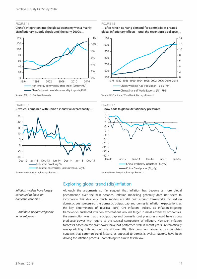
China’s integration into the global economy has affected the world on both the supply and the demand side: China amply supplied labour at low wages, and in many labor-intensive segments, it has achieved a leading market position (even if, more recently, it has started to shift out of them as part of its transition from export- and investment-driven growth toward consumption-led growth). Shifting resources across and within sectors also led to a surge in China’s manufacturing productivity. During the 2000s, it became a major (and often dominant) importer of commodities. And with incomes on the rise, China’s appetite for capital and consumer goods produced abroad has also expanded rapidly.
These supply- and demand-side effects also affected other countries’ inflation rates and contributed to the observed stronger co-movement of inflation worldwide:
• Supply effects: China’s low-cost production created downward pressure on import prices and profit margins abroad (as a consequence of competitive pressures), implying disinflationary effects globally.
• Demand effects: China’s rising demand, particularly for commodities, affected foreign prices through rising export and commodity prices, implying inflationary effects globally.
Research on these effects seems to reflect the different stages in China’s development. Earlier studies based on 1993-2002 data suggest supply effects dominated during this period, with China exports contributing to global disinflation.3 Later studies, using 2002-11 data, find that both Chinese supply and demand shocks significantly affected prices in other countries through direct channels (ie, import and export prices) and indirect ones (ie, exposure to foreign competition and commodity prices), but that the demand shocks mattered more.4 Given the China-driven global commodity price boom of 2002-11, this result does not surprise us.
But things have changed significantly since 2011: China’s marked growth slowdown since then and the collapse in commodity prices suggest the demand shock has reversed, with China now contributing to global disinflation. A successful transition by China toward a consumer- and service-sector-driven growth model, implying a lower savings rate, should eventually lead to increased Chinese demand for non-commodity imports. Similarly, as it moves past its ‘Lewis turning point’ and wages rise further, the disinflationary supply-side effects should also fade. However, while such changes could eventually turn China into a global inflationary force, the interim looks quite different: its permanently reduced demand for commodities (after having previously spurred investments in the expansion of commodity supply), its large overcapacity in ‘old’ industries (eg, steel), and demand-dampening effects from the large debt accumulation of recent years all suggest that China will exert deflationary effects on the world for some time.
3 S Kamin, M. Narazzi, J. Schindler: Is China “Exporting Deflation”?, International Finance Discussion Papers, Board of Governors of the Federal Reserve System, No 791, Jan 2004. 4 Eickmeier and Kühnlenz: China’s role in global inflation dynamics; Discussion paper, Deutsche Bundesbank No 07/2013.
China’s integration into the global economy implied immense supply and demand shocks
Deflationary supply side effects dominated the earlier phase…
…while inflationary effects from strong (commodity) demand dominated in the years up to 2011 Since then, China has become a global disinflationary force
Barclays | Equity Gilt Study 2016
3 March 2016 11
FIGURE 14 China’s integration into the global economy was a mainly disinflationary supply shock until the early 2000s…
FIGURE 15 … after which its rising demand for commodities created global inflationary effects – until the recent price collapse…
Source: IMF, UN, Barclays Research Source: UNComtrade, World Bank, Barclays Research
FIGURE 16 ... which, combined with China’s industrial overcapacity,…
FIGURE 17 …now adds to global deflationary pressures
Source: Haver Analytics, Barclays Research Source: Haver Analytics, Barclays Research
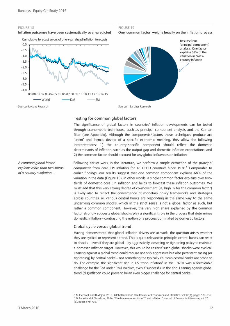
Exploring global trend (dis)inflation Although the arguments so far suggest that inflation has become a more global phenomenon over the past decades, inflation modelling generally does not seem to incorporate this idea very much: models are still built around frameworks focused on domestic cost pressures, the domestic output gap and domestic inflation expectations as the key determinants of (cyclical core) CPI inflation. Indeed, as inflation-targeting frameworks anchored inflation expectations around target in most advanced economies, the assumption was that the output gap and domestic cost pressures should have strong predictive power with regard to the cyclical component of inflation. However, inflation forecasts based on this framework have not performed well in recent years, systematically over-predicting inflation outturns (Figure 18). This common failure across countries suggests that common trend factors, as opposed to domestic cyclical factors, have been driving the inflation process – something we aim to test below.
0%
2%
4%
6%
8%
10%
12%
0
20
40
60
80
100
120
140
1994 1998 2002 2006 2010 2014
Non-energy commodity price index (2010=100)
China's share in world commodity imports; RHS
0
2
4
6
8
10
12
14
500
600
700
800
900
1,000
1,100
1978 1982 1986 1990 1994 1998 2002 2006 2010 2014
China: Working Age Population 15-65 (mn)
China: Share of World Exports (%) RHS
-10
-5
0
5
10
15
20
25
Dec-12 Jun-13 Dec-13 Jun-14 Dec-14 Jun-15 Dec-15Industrial Profit,y/y %Industrial enterprises: Sales revenue, y/y%
-40
-35
-30
-25
-20
-15
-10
-5
0
5
10
Jan-11 Jan-12 Jan-13 Jan-14 Jan-15 Jan-16
China: PPI heavy industries (%, y/y)
China: Steel prices (%, y/y)
Inflation models have largely continued to focus on domestic variables… …and have performed poorly in recent years
Barclays | Equity Gilt Study 2016
3 March 2016 12
FIGURE 18 Inflation outcomes have been systematically over-predicted
FIGURE 19 One ‘common factor’ weighs heavily on the inflation process
Source: Barclays Research Source: Barclays Research
Testing for common global factors The significance of global factors in countries’ inflation developments can be tested through econometric techniques, such as principal component analysis and the Kalman filter (see Appendix). Although the components/factors these techniques produce are ‘latent’ and, hence, devoid of a specific economic meaning, they allow the following interpretations: 1) the country-specific component should reflect the domestic determinants of inflation, such as the output gap and domestic inflation expectations; and 2) the common factor should account for any global influences on inflation.
Following earlier work in the literature, we perform a simple extraction of the principal component from core CPI inflation for 16 OECD countries since 1976.5 Comparable to earlier findings, our results suggest that one common component explains 68% of the variation in the data (Figure 19); in other words, a single common factor explains over two-thirds of domestic core CPI inflation and helps to forecast these inflation outcomes. We must add that this very strong degree of co-movement (ie, high % for the common factor) is likely also to reflect the convergence of monetary policy frameworks and strategies across countries: ie, various central banks are responding in the same way to the same underlying common shocks, which in the strict sense is not a global factor as such, but rather a common component. However, the very high share explained by the common factor strongly suggests global shocks play a significant role in the process that determines domestic inflation – contrasting the notion of a process dominated by domestic factors.
Global cycle versus global trend Having demonstrated that global inflation drivers are at work, the question arises whether they are cyclical or represent a trend. This is quite relevant: in principle, central banks can react to shocks – even if they are global – by aggressively loosening or tightening policy to maintain a domestic inflation target. However, this would be easier if such global shocks were cyclical. Leaning against a global trend could require not only aggressive but also persistent easing (or tightening) by central banks – not something the typically cautious central banks are prone to do. For example, the significant rise in US trend inflation6 in the 1970s was a formidable challenge for the Fed under Paul Volcker, even if successful in the end. Leaning against global trend (dis)inflation could prove to be an even bigger challenge for central banks.
5 M Ciccarelli and B Mojon, 2010, ‘Global Inflation’, The Review of Economics and Statistics, vol 92(3), pages 524-535. 6 G Ascari and A Sbordone, 2014, “The Macroeconomics of Trend Inflation”, Journal of Economic Literature, vol 52 (3), pages 679-739.
-4.0
-3.5
-3.0
-2.5
-2.0
-1.5
-1.0
-0.5
0.0
00 00 01 02 03 04 05 05 06 07 08 09 10 10 11 12 13 14 15
World DM EM
Cumulative forecast errors of one-year ahead inflation forecasts Results from 'principal component' analysis: One factorexplains 68% of the variation in cross-country Inflation
A common global factor explains more than two-thirds of a country’s inflation…

Barclays | Equity Gilt Study 2016
3 March 2016 13
The phenomenon of trend inflation has been examined in some studies on the US, but not yet across OECD countries. We undertake this exercise with a Dynamic Common Factor model and decompose the trend from cycle inflation factors. We estimate the following model on core CPI inflation series for 16 OECD countries:
𝜋𝑖,𝑡 = 𝛼𝑖𝐶𝑡 + 𝛽𝑖𝑇𝑡 + 𝛿𝑗𝑋𝑖,𝑡 + 𝑒𝑖 ,𝑡
In this model, 𝜋𝑖,𝑡 is quarterly inflation in country i. This is explained by a cyclical (𝐶𝑡) and trend component (𝑇𝑡). The trend is modelled as a random walk and we impose a prior condition that it can evolve only slowly.7 The cyclical component, on the other hand, is assumed to have zero persistence.8
The model results for the global cyclical factor (𝐶𝑡) should reflect the global business cycle and global commodity price shocks.9 Indeed, we find a clear rise in the global cyclical factor in the late 1980s boom and a decline during the 1991, 2001 and 2008-09 recessions.10 Notably, the 1991 Q1 peak in the global cyclical factor occurs after the 132% rise in Brent crude between Q2 and Q3 90. Subsequent peaks coincide with the early 2000s and 2007-09.
The model’s global trend component (Tt) should reflect such factors as permanent policy or behavioural changes, including inflation expectations. Similarly, it can also be interpreted as the medium-term level of inflation that – after all shocks have died out – is consistent with a given monetary policy. Indeed, our findings show a sharp fall in the trend inflation factor from 6.3% annualised inflation in the 1980s, consistent with a shift in inflation expectations around this time (Figure 20). A further decline occurs in the mid-1990s, broadly coinciding with the global adoption of inflation targeting and ongoing convergence in Europe ahead of the introduction of the euro. Importantly, there is also a drop in trend inflation in Q3 08, from 1.6% to 1.2% and in 2012, from 1.32% to 1.00% at the end of the sample. As shown in the appendix, our model suggests that both these breaks are statistically significant.
These two recent breaks lower in global trend inflation coincide with the global financial crisis (2008-09) and the euro area crisis (2011-12), as shown in Figure 21. Intuitively, the trend breaks suggest that either inflation expectations shifted down or that the monetary policy
7 T Cogley, G Primiceri and T Sargent, 2010, “Inflation-Gap persistence in the US”, American Economic Journal: Macroeconomics, vol 2(1), pages 43-69. 8 In a recent study on US trend inflation, Stock and Watson (2015) argue that this is a necessary assumption to allow the separation of these two factors. 9 As detailed in the Appendix, for the econometric exercise, ‘cyclical’ is defined as the component having zero persistence. 10 While 1991, 2001 and 2009 are US recessions as defined by the NBER, the 1991 and 2009 recession are also global recessions—two of the four global recessions since 1960—as defined by recent work of the IMF: When National Cycles Coincide: Tracking Global Recessions and Recoveries IMF Survey February 9, 2016.
FIGURE 20 The global trend inflation factor has continued to fall…
FIGURE 21 …with two further ‘breaks’ in 2008/9 and 2011/12
Source: Barclays Research Source: Barclays Research
…and this global factor has a declining trend component
0.0
1.0
2.0
3.0
4.0
5.0
6.0
7.0
Q4-83 Q4-87 Q4-91 Q4-95 Q4-99 Q4-03 Q4-07 Q4-11 Q4-15
World trend inflation factor (%, quarterly anualized)
0.5
0.7
0.9
1.1
1.3
1.5
1.7
1.9
2.1
Q4-01 Q4-03 Q4-05 Q4-07 Q4-09 Q4-11 Q4-13 Q4-15
World trend inflation factor (%, quarterly anualized)
Euro area crisis
Global financial crisis
Barclays | Equity Gilt Study 2016
3 March 2016 14
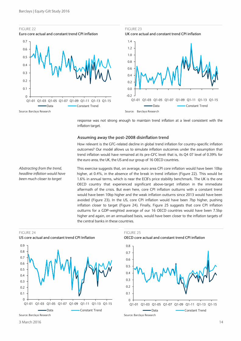
response was not strong enough to maintain trend inflation at a level consistent with the inflation target.
Assuming away the post-2008 disinflation trend How relevant is the GFC-related decline in global trend inflation for country-specific inflation outcomes? Our model allows us to simulate inflation outcomes under the assumption that trend inflation would have remained at its pre-GFC level: that is, its Q4 07 level of 0.39% for the euro area, the UK, the US and our group of 16 OECD countries.
This exercise suggests that, on average, euro area CPI core inflation would have been 10bp higher, at 0.4%, in the absence of the break in trend inflation (Figure 22). This would be 1.6% in annual terms, which is near the ECB’s price stability benchmark. The UK is the one OECD country that experienced significant above-target inflation in the immediate aftermath of the crisis. But even here, core CPI inflation outturns with a constant trend would have been 10bp higher and the weak inflation outturns since 2013 would have been avoided (Figure 23). In the US, core CPI inflation would have been 7bp higher, pushing inflation closer to target (Figure 24). Finally, Figure 25 suggests that core CPI inflation outturns for a GDP-weighted average of our 16 OECD countries would have been 7.5bp higher and again, on an annualised basis, would have been closer to the inflation targets of the central banks in these countries.
FIGURE 22 Euro core actual and constant trend CPI inflation
FIGURE 23 UK core actual and constant trend CPI inflation
Source: Barclays Research Source: Barclays Research
Abstracting from the trend, headline inflation would have been much closer to target
FIGURE 24 US core actual and constant trend CPI Inflation
FIGURE 25 OECD core actual and constant trend CPI inflation
Source: Barclays Research Source: Barclays Research
0
0.1
0.2
0.3
0.4
0.5
0.6
0.7
Q1-01 Q1-03 Q1-05 Q1-07 Q1-09 Q1-11 Q1-13 Q1-15
Data Constant Trend
-0.2
0.0
0.2
0.4
0.6
0.8
1.0
1.2
1.4
Q1-01 Q1-03 Q1-05 Q1-07 Q1-09 Q1-11 Q1-13 Q1-15
Data Constant Trend
0
0.1
0.2
0.3
0.4
0.5
0.6
0.7
0.8
0.9
Q1-01 Q1-03 Q1-05 Q1-07 Q1-09 Q1-11 Q1-13 Q1-15
Data Constant Trend
0
0.1
0.2
0.3
0.4
0.5
0.6
0.7
0.8
Q1-01 Q1-03 Q1-05 Q1-07 Q1-09 Q1-11 Q1-13 Q1-15
Data Constant Trend

Barclays | Equity Gilt Study 2016
3 March 2016 15
Our interim summary is that: 1) domestic inflation processes seem significantly influenced by a common global factor; 2) the trend component of this global inflation factor has been declining, from very high levels, since the early 1980s, but it has dropped further since the global financial crisis (GFC) and the euro area crisis; and 3) without this trend decline, domestic inflation outcomes would have been closer to official targets in recent years, particularly in the euro area.
Reconsidering ‘global’ versus ‘coincidence of domestic’ factors So far, we have argued that there has been a significant global trend in domestic inflation outturns since the 1980s. This appears to have undergone further structural breaks in 2008 and 2012. Our results suggest that this has led to weaker core CPI inflation outturns in OECD countries. However, as we highlighted at the outset, one challenge to our econometric approach is that this extracted trend common factor is an unobserved variable. Hence, we cannot exclude that a mere coincident move of domestic factors might be responsible for the shift in the global trend.
To explore this hypothesis further, particularly for the 2008 and 2012 trend breaks, we include a number of domestic exogenous variables in our model. These are the domestic output gap, quarterly/annual growth of wages, unit labour costs, real credit, property prices and labour productivity, the NAIRU, and the unemployment rate. For the output gap measures, we explore different options. Our baseline measure for the output gap is the Hodrick-Prescott filtered measure of domestic real GDP. However, we also test the OECD’s model-based output gap and try an output gap measure suggested by Borio et al (2014) that adjusts for demand weakness since the GFC, including real interest rates, real credit growth and real house price growth in the output gap measure. Finally, as long-run trends in core inflation might also be determined by the spending patterns of different demographic groups, we include population growth and old-age dependency ratios to account for these effects.
Given the large number of variables we examine, we adopt the following investigative strategy: we include the output gap and population growth and old-age dependency ratios to account for the standard cyclical and trend determinants of inflation in every specification. We then add each one of our proposed variables one-by-one to examine if any one is an important determinant of trend inflation. When we explore alternative measures of spare capacity such as the financially adjusted output gap or the NAIRU, we replace these variables with the standard output gap.
In addition, we want to test whether the global counterparts of the above variables may matter more than the domestic ones. We therefore also include the corresponding global variables, which we construct as the GDP-weighted averages of the country-specific variables. To test whether the effect of spare capacity on prices is mainly transmitted through trade between countries (eg, for Canada, the US output gap is most likely significantly more important than implied by GDP-weights) we also include trade-weighted averages of slack in a country’s trading partners.
It turns out that among all these candidate variables, domestic labour market variables are most significant. Indeed, allowing domestic unit labour costs growth rates to enter in our econometric model leads to a flat global trend inflation component in 2008-12.11 Although it may seem odd that domestic variables can explain a global factor, this presumably reflects the fact that a sharp increase in labour market slack coincided across OECD countries following the deep global recession associated with the GFC. However, domestic labour market variables alone still cannot explain the further decline in trend inflation since 2012. Adding global output gap measures cannot explain this last decline, either. Only when we include global annual wage growth, weighted by trading partner into our model, does the recent
11 In our baseline model, the output gap, population growth and the old-age dependency ratio are always included. We explore the importance of the other variables by including them one-by-one.
Exploring the ‘unobserved’ common factor by re-introducing global and domestic variables
We include trade-weighted averages to investigate the potential cross-border transmission of slack

Barclays | Equity Gilt Study 2016
3 March 2016 16
break in the trend disappear. This suggests the presence of another global trend, in common to prices and wages, that is likely responsible for this last trend break in inflation.
To examine this idea, we then estimate the global trend in quarterly wage growth rates for our sample of countries and compare with global CPI trend inflation. This suggests that historically, the global trend in wage inflation leads the CPI trend inflation factor by about a year (Figure 26)12. Since the GFC, the global wage trend inflation factor has remained weak, which is likely to keep global CPI trend inflation weak for some time (Figure 27).
Overall, these final findings about the post-GFC period suggest that: 1) both local and global labour market factors have been important determinants of trend inflation since 2008; 2) therefore, labour market variables in general seem to have become the most relevant concept of economic slack in recent years; and 3) global wage weakness is likely to keep CPI trend inflation low for some time to come.
Implications for monetary policy and beyond The global disinflation trend since the 1980s is explained by a number of factors, including changes in monetary policy regimes, domestic deregulation, and the effects of technological advances combined with increased global flows of goods, services and capital. This globalization, accelerated by the integration of China into the world economy, has meant that global drivers have gained in relevance compared with the domestic drivers of inflation in a given country. Our findings suggest that the common global factor is not merely cyclical (ie, business cycles) or a proximate driver (ie, oil price swings) but includes a significant trend component that has been trending lower. They also show that this trend component has shifted down further since the GFC (2008-09) and the euro area crisis (2011-12), suggesting it may be the main driver of the below-target inflation in advanced economies.
Such a global disinflationary trend is challenging news for central banks mandated to keep inflation around certain annual targets (ie, 2% for most of them). Does it imply that central banks are no longer in control of their domestic inflation developments? In other words, has their mission become impossible?
12 Indeed, standard tests suggest that these variables are co-integrated.
FIGURE 26 Wage inflation tended to lead trend CPI inflation …
FIGURE 27 …but wage inflation has remained very weak since the GFC
Source: Barclays Research Source: Barclays Research
Labor markets matter most for recent decline in trend inflation
Central banks face a challenge: the trend is not their friend
Has inflation-targeting become a ‘mission impossible’?
-1.0
0.0
1.0
2.0
3.0
4.0
5.0
6.0
Q4-91 Q4-95 Q4-99 Q4-03 Q4-07 Q4-11 Q4-15
Global wage trend inflation factor (%, quarterly annualized)
Global CPI trend inflation factor (%, quarterly annualized)
0.5
1.0
1.5
2.0
2.5
3.0
3.5
-1.0
0.0
1.0
2.0
3.0
4.0
5.0
6.0
7.0
Q4-91 Q4-95 Q4-99 Q4-03 Q4-07 Q4-11 Q4-15
Global wage trend inflation factor (%, quarterly annualized)
Global CPI trend inflation factor (%, quart. annualized) RHS

Barclays | Equity Gilt Study 2016
3 March 2016 17
Our findings suggest a nuanced answer. First, a closer look at drivers of the disinflation trend in the post-GFC period suggests that domestic and global labour market variables have both been significant. Indeed, technically it remains difficult to distinguish truly ‘global’ from ‘coincident domestic’ factors. Second, the global trend in wage inflation has historically been a powerful leading indicator of the global trend in core CPI inflation. The recent weakness in the former suggests that CPI trend inflation is likely to remain low for some time to come. However, the breaks in the trend component do seem related to monetary policy changes: declines in trend inflation seem to have followed rises in OECD monetary policy rates (Figure 28). The most recent break, in 2012, occurred after the ECB’s policy rate increase in Q2 and Q3 11, suggesting that the tightening of monetary policy in the euro area played a role in shifting global trend inflation lower (Figure 29).
Taken together, the following conclusions seem to emerge: monetary policy may not be powerless, but with domestic inflation outcomes exposed to global factors beyond its control, the disinflationary trend it faces may simply be too strong for the policies central banks have been willing to deploy. In other words, monetary policy has simply not been loose enough for the slack, in particular in labour markets, created by the GFC, which is in line with our analysis in Chapter 2, “When absolute zero isn’t low enough”. Almost certainly a consequence of globalization, monetary policies in core economies seem to affect the global trend component. Thus, for example, the ECB’s rate hikes in 2011 – later revised –seem to have affected our global inflation measure. How global trend inflation could be affected by the Federal Reserve’s current hiking cycle remains to be seen. But the ECB’s experience suggests that a potential policy mistake by the Fed of premature or too aggressive hikes could worsen global trend inflation further.
This suggests that: 1) central banks may have to be even more aggressive and persistent to lean against the powerful disinflation trend; and 2) that they must take into account the policies of others, as these can spill over into their own inflation outlook (and vice versa). These suggestions come with formidable challenges, however. Aggressively and persistently leaning against a trend was difficult for the Fed in the 1980s, when the trend was for rising inflation and the response was obvious (tightening through higher rates). Now, the trend is for disinflation and the necessary policy response of easing is constrained by the zero lower bound (ZLB). However, our findings suggest that central banks may have to continue down this path to turn the disinflation trend around. Given the above-mentioned spill-overs, they ideally should do this in a coordinated manner, in awareness of the effect their policies have elsewhere. Indeed, the simultaneous cuts by core central banks early on during the GFC and the subsequent pursuit of QE by the Fed and the BoE could be considered as an example of a successful simultaneous policy move.
FIGURE 28 Trend inflation and OECD monetary policy
FIGURE 29 Trend inflation and ECB refinancing rate
Source: Barclays Research Source: Barclays Research
Domestic labor market variables are still significant … …and monetary policy seems to affect trend inflation…
… but it has become harder for central bankers to achieve their desired outcome … … and the actions of others now matter more
Policies have to be ‘aggressive and persistent’… …and the policies of others must be taken into account… … and, ideally, should be coordinated
0.0
0.2
0.4
0.6
0.8
1.0
1.2
1.4
1.6
1.8
0.0
2.0
4.0
6.0
8.0
10.0
12.0
Q4-83 Q1-90 Q2-96 Q3-02 Q4-08 Q1-15
OECD Country policy rate (LHS) Trend inflation (RHS)
0.0
0.1
0.2
0.3
0.4
0.5
0.6
0.0
0.5
1.0
1.5
2.0
2.5
3.0
3.5
4.0
4.5
5.0
Q1-00 Q1-05 Q1-10 Q1-15
ECB Main Refi Rate (LHS) Trend inflation (RHS)

Barclays | Equity Gilt Study 2016
3 March 2016 18
The need to be aggressive and persistent seems to have now been accepted by most central banks, judging not only by the QE programs but also by the more recent moves by a number of central banks to challenge the ZLB and move policy rates into negative territory. We explore the consequences of such policies in more depth in Chapter 3, “Negative Ascent: Life amid negative nominal interest rates”. In addition, the Fed’s very cautious attitude toward hiking its policy rate suggests an increased recognition of global spill-over effects, even if this comes from the perspective of how other countries (eg, China) affect US inflation, rather than how US policy would affect theirs. An active coordination of policies – which would be complicated by having to include exchange rate considerations – may ultimately require a more urgent sense of crisis.
Last, our analysis is purely concerned with inflation and monetary policies’ effect on it. However, aggressive and persistent monetary easing, including with unconventional policies, to overcome a strong disinflation trend can also have significant unintended consequences for financial stability. And to the extent that financial instability could cause further global disinflationary shocks down the line, such a policy could become counter-productive. In principle, this points toward the need for support from fiscal and/or structural policies. Indeed, this is something the ECB and other central banks have been asking for, albeit with limited success. Without this support, but a mandate to bring inflation to target, central bankers will have to continue testing the extremes. For investors, this means that: 1) financial volatility is likely here to stay; and 2) although there is little to suggest a turn in global inflation anytime soon, when it does happen, the unwinding of these policies could be challenging.
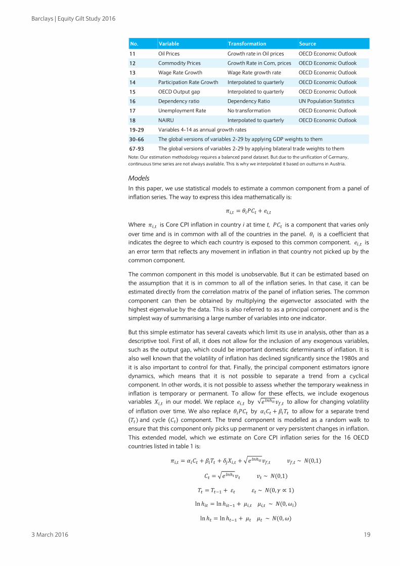
Appendix: Data and Models Data In this appendix, we first describe the data and then the two models that we estimate on the dataset. Table 1 shows the list of countries in our sample, while Table 2 shows the variables in our model.
TABLE 1 List of countries
Australia Germany Sweden
Austria Italy Switzerland
Canada Japan US
Denmark Netherlands UK
Finland Luxembourg
France Spain
Note: This list of countries was constrained by the availability of core CPI inflation data. We included all OECD countries were data was available starting in 1976Q3.
TABLE 2 List of variables
No. Variable Transformation Source
1 Core CPI Inflation Growth rate of Core CPI OECD Economic Outlook
2 Output Gap HP-filtered log of real GDP OECD Economic Outlook
3 Real Interest Rates Policy rate – CPI inflation OECD Economic Outlook
4 House Price Growth Growth rate of real credit BIS
5 Real Credit Growth Growth rate of real credit BIS
6 Population Growth 5-year Growth Pop. Growth UN Population Statistics
7 Labour Productivity Growth Growth in Output/Employee OECD Economic Outlook
8 Labour Productivity Growth Growth in Output/Hour OECD Economic Outlook
9 Unit Labour Costs Growth Growth rate in ULC OECD Economic Outlook
10 Real Exchange Rates Growth rate in RFX OECD Economic Outlook
Negative policy rates may become a fixture of the menu
But policies to bring back inflation also bring financial stability risk… ...leaving central bankers in a bind and investors in a volatile environment
Barclays | Equity Gilt Study 2016
3 March 2016 19
No. Variable Transformation Source
11 Oil Prices Growth rate in Oil prices OECD Economic Outlook
12 Commodity Prices Growth Rate in Com, prices OECD Economic Outlook
13 Wage Rate Growth Wage Rate growth rate OECD Economic Outlook
14 Participation Rate Growth Interpolated to quarterly OECD Economic Outlook
15 OECD Output gap Interpolated to quarterly OECD Economic Outlook
16 Dependency ratio Dependency Ratio UN Population Statistics
17 Unemployment Rate No transformation OECD Economic Outlook
18 NAIRU Interpolated to quarterly OECD Economic Outlook
19-29 Variables 4-14 as annual growth rates
30-66 The global versions of variables 2-29 by applying GDP weights to them
67-93 The global versions of variables 2-29 by applying bilateral trade weights to them
Note: Our estimation methodology requires a balanced panel dataset. But due to the unification of Germany, continuous time series are not always available. This is why we interpolated it based on outturns in Austria.
Models In this paper, we use statistical models to estimate a common component from a panel of inflation series. The way to express this idea mathematically is:
𝜋𝑖,𝑡 = 𝜃𝑖𝑃𝐶𝑡 + 𝑒𝑖,𝑡
Where 𝜋𝑖,𝑡 is Core CPI inflation in country i at time t, 𝑃𝐶𝑡 is a component that varies only
over time and is in common with all of the countries in the panel. 𝜃𝑖 is a coefficient that indicates the degree to which each country is exposed to this common component. 𝑒𝑖 ,𝑡 is an error term that reflects any movement in inflation in that country not picked up by the common component.
The common component in this model is unobservable. But it can be estimated based on the assumption that it is in common to all of the inflation series. In that case, it can be estimated directly from the correlation matrix of the panel of inflation series. The common component can then be obtained by multiplying the eigenvector associated with the highest eigenvalue by the data. This is also referred to as a principal component and is the simplest way of summarising a large number of variables into one indicator.
But this simple estimator has several caveats which limit its use in analysis, other than as a descriptive tool. First of all, it does not allow for the inclusion of any exogenous variables, such as the output gap, which could be important domestic determinants of inflation. It is also well known that the volatility of inflation has declined significantly since the 1980s and it is also important to control for that. Finally, the principal component estimators ignore dynamics, which means that it is not possible to separate a trend from a cyclical component. In other words, it is not possible to assess whether the temporary weakness in inflation is temporary or permanent. To allow for these effects, we include exogenous variables 𝑋𝑖,𝑡 in our model. We replace 𝑒𝑖 ,𝑡 by √𝑒𝑙𝑛ℎ𝑖𝑡𝑣𝑓,𝑡 to allow for changing volatility
of inflation over time. We also replace 𝜃𝑖𝑃𝐶𝑡 by 𝛼𝑖𝐶𝑡 + 𝛽𝑖𝑇𝑡 to allow for a separate trend (𝑇𝑡) and cycle (𝐶𝑡) component. The trend component is modelled as a random walk to ensure that this component only picks up permanent or very persistent changes in inflation. This extended model, which we estimate on Core CPI inflation series for the 16 OECD countries listed in table 1 is:
𝜋𝑖,𝑡 = 𝛼𝑖𝐶𝑡 + 𝛽𝑖𝑇𝑡 + 𝛿𝑗𝑋𝑖,𝑡 + �𝑒𝑙𝑛ℎ𝑖𝑡𝑣𝑓,𝑡 𝑣𝑓,𝑡 ~ 𝑁(0,1)
𝐶𝑡 = �𝑒𝑙𝑛ℎ𝑡𝑣𝑡 𝑣𝑡 ~ 𝑁(0,1)
𝑇𝑡 = 𝑇𝑡−1 + 𝜀𝑡 𝜀𝑡 ~ 𝑁(0,𝛾 ∝ 1)
lnℎ𝑖𝑡 = lnℎ𝑖𝑡−1 + 𝜇𝑖,𝑡 𝜇𝑖,𝑡 ~ 𝑁(0,𝜔𝑖)
lnℎ𝑡 = lnℎ𝑡−1 + 𝜇𝑡 𝜇𝑡 ~ 𝑁(0,𝜔)
Barclays | Equity Gilt Study 2016
3 March 2016 20
In this model, 𝜋𝑖,𝑡 is quarterly inflation in country i. This is explained by a cyclical (𝐶𝑡) and trend component (𝑇𝑡 ), as well as a vector of exogenous variables 𝑋𝑖,𝑡 . The cyclical component, on the other hand, is assumed to have zero persistence.13 The trend is modelled as a random walk and we impose a prior that it can only evolve slowly over time.14 Specifically, we impose a prior that 𝛾, is .0001, meaning that the trend can only move by one percent of the standard deviation at a time. Cogely, Primiceri and Sargent (2010) argue that setting the prior in this manner will ensure that the trend component only picks up permanent structural change. We also allow the variances of the model to vary over time via ℎ𝑖𝑡 and ℎ𝑡. This is an important model feature as it picks up the changed in inflation volatility over time. Clearly, interpreting any regression with all 92 potential explanatory variables listed in table 1 will be challenging. For this reason, we investigate the explanatory power of these variables one by one. But our model does include several standard determinants of the inflation trend and cycle in each regression. These are the output gap, population growth and the dependency ratio. To estimate the model, we cast the model into State Space form and use Bayesian Kalman filter with Gibbs sampling to estimate the model.
For the aficionado Other than separating the trend from the cycle, a challenge in unobserved components models is the separation of the scale of the trend and cycle factors. In particular, one could multiply both 𝛼𝑖 and 𝐶𝑡 by 1
2 each, that model would be observationally equivalent to the
model described above. To address the scaling issue, we use a standard solution and fix the scale of the variance of both the trend and the cycle to 1. This determines the scale of the factors and therefore also the coefficients.
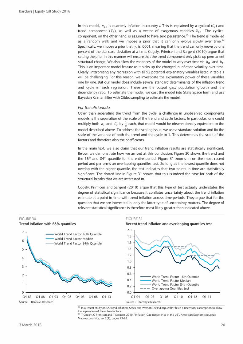
In the main text, we also claim that our trend inflation results are statistically significant. Below, we demonstrate how we arrived at this conclusion. Figure 30 shows the trend and the 16th and 84th quantile for the entire period. Figure 31 zooms in on the most recent period and performs an overlapping quantiles test. So long as the lowest quantile does not overlap with the higher quantile, the test indicates that two points in time are statistically significant. The dotted line in Figure 31 shows that this is indeed the case for both of the structural breaks that we are interested in.
Cogely, Primiceri and Sargent (2010) argue that this type of test actually understates the degree of statistical significance because it conflates uncertainty about the trend inflation estimate at a point in time with trend inflation across time periods. They argue that for the question that we are interested in, only the latter type of uncertainty matters. The degree of relevant statistical significance is therefore most likely greater than indicated above.
13 In a recent study on US trend inflation, Stock and Watson (2015) argue that his is a necessary assumption to allow the separation of these two factors. 14 T Cogley, G Primiceri and T Sargent, 2010, “Inflation-Gap persistence in the US”, American Economic Journal: Macroeconomics, vol 2(1), pages 43-69.
FIGURE 30 Trend inflation with 68% quantiles
FIGURE 31 Recent trend inflation and overlapping quantiles test
Source: Barclays Research
Source : Barclays Research
0
1
2
3
4
5
6
7
Q4-83 Q4-88 Q4-93 Q4-98 Q4-03 Q4-08 Q4-13
World Trend Factor 16th QuantileWorld Trend Factor MedianWorld Trend Factor 84th Quantile
0.0
0.2
0.4
0.6
0.8
1.0
1.2
1.4
1.6
1.8
2.0
Q1-04 Q1-06 Q1-08 Q1-10 Q1-12 Q1-14
World Trend Factor 16th QuantileWorld Trend Factor MedianWorld Trend Factor 84th QuantileOverlapping Quantiles test

Barclays | Equity Gilt Study 2016
3 March 2016 21
References Ascari,G. and A. Sbordone. 2014. “The macroeconomics of trend inflation.” Journal of Economic Literature, vol 52 (3), pages 679-739.
Bank For International Settlements (BIS). 2015. 85th Annual Report
Bean, Charlie. 2006. Globalisation and Inflation. Quarterly Bulletin 2006 Q4
Borio, Claudio and Andrew Filardo. 2007. “Globalisation and inflation: New cross-country evidence on the global determinants of domestic inflation.” BIS, Working paper no 227.
Borio, Claudio, Piti Disyatata and Mikael Juselius. 2013. “Rethinking potential output: Embedding information about the financial cycle.” BIS, Working paper no 404.
Calza, Alessandro. 2008. “Globalisation, domestic inflation and global output gaps-Evidence from the euro area.” European Central Bank, Working Paper Series.
Ciccarelli, Matteo and Benoit Mojon. 2010. “Global inflation.” The Review of Economics and Statistics, vol 92(3), pages 524-535.
Cogley, T., G. Primiceri and T Sargent. 2010. “Inflation-gap persistence in the US.” American Economic Journal: Macroeconomics, vol 2(1), pages 43-69.
Cogley, Timothy, and Argia M. Sbordone. 2008. “Trend inflation, indexation and inflation persistence in the New Keynesian Phillips Curve.” American Economic Review: Vol 98 No 5.
Constancio, Vitor. 2015. “Understanding inflation dynamics and monetary policy.” IMF Working Paper No. 11/121.
Eickmeier and Kühnlenz. 2013. “China’s role in global inflation dynamics.” Deutsche Bundesbank, Discussion paper No 07/2013.
Eickmeier, Sandra and Katharina Moll. 2009. “The Global dimension of inflation - Evidence from factor augmented Phillips Curves.” European Central Bank, Working Paper Series.
Ferroni, Filippo and Benoit Mojon. 2014. “Domestic and global inflation.” http://www.benoitmojon.com/pdf/FerroniMojon_v9.pdf .
Friedrich, Christian. 2014. “Global inflation dynamics in the post-crisis period: What explains the twin puzzle.” Bank of Canada, Working Paper 2014-36.
Gerard, Hugo. 2012. “Comovement in inflation.” Reserve Bank of Australia.
Hakkio, Craig. 2009. “Global inflation dynamics.” The Federal Reserve Bank of Kansas City.
Helbling, Thomas, Florence Jaumotte, and Martin Sommer. 2006. “How has globalization affected inflation?” IMF WEO April 2006, Chapter III.
Ihrig, Jane, Steven B. Kamin, Deborah Lindner and Jaime Marquez. 2007. “Some simple tests of the globalization and inflation hypothesis.” Board of Governors of the Federal Reserve System, International Finance Discussion Papers, no. 891.
Kamin, Steven B., Mario Marazzi and John W. Schindler. 2004. “Is China exporting deflation?” Board of Governors of the Federal Reserve System, International Finance Discussion Papers, no. 791.
Martinez-Garcia, Enrique and Mark A Wynne. 2012. “Global slack as a determinant of US inflation.” Federal Reserve Bank of Dallas, Globalization and Monetary Policy Institute, Working Paper No. 123.
Mazumder, Sandeep and Laurence M Ball. 2011. “Inflation Dynamics and the Great Recession.” IMF Working Paper No. 11/121.

Barclays | Equity Gilt Study 2016
3 March 2016 22
Murphy, Robert G. 2013. “Explaining Inflation in the aftermath of the Great Recession.” Journal of Macroeconomics, Volume 40.
Nelly, Christopher J. and David E Rapach. 2011. “International comovements in inflation rates and country characteristics.” Federal Reserve Bank of St. Louis, Working Paper Series.
Stock, James and Mark Watson. 2012. “Disentangling the Channels of the 2007-2009 Recession” May 2012, Brookings Papers on Economic Activity, Spring 2012.
Stock, James H. and Mark W. Watson. Forthcoming. “Core inflation and trend Inflation.” Review of Economics and Statistics.
White, William R. 2008. “Globalisation and the determinants of domestic inflation.” BIS Working Papers, no. 250.
Barclays | Equity Gilt Study 2016
3 March 2016 23
CHAPTER 2
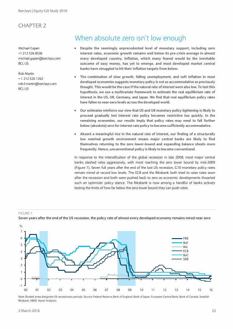
When absolute zero isn’t low enough • Despite the seemingly unprecedented level of monetary support, including zero
interest rates, economic growth remains well below its pre-crisis average in almost every developed country. Inflation, which many feared would be the inevitable outcome of easy money, has yet to emerge, and most developed market central banks have struggled to hit their inflation targets from below.
• The combination of slow growth, falling unemployment, and soft inflation in most developed economies suggests monetary policy is not as accommodative as previously thought. This would be the case if the natural rate of interest were also low. To test this hypothesis, we use a multivariate framework to estimate the real equilibrium rate of interest in the US, UK, Germany, and Japan. We find that real equilibrium policy rates have fallen to near-zero levels across the developed world.
• Our estimates reinforce our view that US and UK monetary policy tightening is likely to proceed gradually lest interest rate policy becomes restrictive too quickly. In the remaining economies, our results imply that policy rates may need to fall further below (absolute) zero for interest rate policy to become sufficiently accommodative.
• Absent a meaningful rise in the natural rate of interest, our finding of a structurally low nominal growth environment means major central banks are likely to find themselves returning to the zero lower-bound and expanding balance sheets more frequently. Hence, unconventional policy is likely to become conventional.
In response to the intensification of the global recession in late 2008, most major central banks slashed rates aggressively, with most reaching the zero lower bound by mid-2009 (Figure 1). Seven full years after the end of the last US recession, G10 monetary policy rates remain mired at record low levels. The ECB and the Riksbank both tried to raise rates soon after the recession and both were pushed back to zero as economic developments thwarted such an optimistic policy stance. The Riksbank is now among a handful of banks actively testing the limits of how far below the zero lower bound they can push rates.
Michael Gapen +1 212 526 8536 [email protected] BCI, US Rob Martin + 1 212 526 1262 [email protected] BCI, US
FIGURE 1 Seven years after the end of the US recession, the policy rate of almost every developed economy remains mired near zero
Note: Shaded areas designate US recessionary periods. Source: Federal Reserve, Bank of England, Bank of Japan, European Central Bank, Bank of Canada, Swedish Riksbank, NBER, Haver Analytics
- 1 0 1 2 3 4 5 6 7
00 01 02 03 04 05 06 07 08 09 10 11 12 13 14 15 16
%
FRB BoE BoJ ECB BoC SRB

Barclays | Equity Gilt Study 2016
3 March 2016 24
Besides pushing rates lower, these central banks expanded their balance sheets substantially. Through various programs, particularly asset purchases, the Fed and the ECB both increased their balance sheets to about 25% of GDP (Figure 2). The Bank of Japan, in a monumental effort to boost the Japanese economy and produce inflation, began an asset purchase program in 2013 that has since ballooned its balance sheet to more than 70% of GDP.
The unprecedented monetary response to the crisis led many academics and policymakers to fear a resurgence of inflation in which central banks would be forced to abruptly tighten policy to bring inflation back to target. Now, as central banks struggle to meet inflation targets from below, concerns have shifted. The absence of inflation now leads many to worry about the fundamental ability of monetary policy to produce it. Add to this that economic growth remains below its pre-crisis average in almost every developed country and the concern deepens. See Chapter 1: The fight to bring back inflation, for a discussion of the implications for the global economy if monetary policy has indeed lost its ability to stimulate either inflation or growth.
In this chapter, we take a different tack. Focusing on four G10 economies – the US, UK, Germany, and Japan – we move beyond simply observing the level of policy rates and attempt to compare the level of the target rate to the evolution of the natural rate of interest. The natural rate, simply put, is the rate of interest that tends to be neutral with respect to both growth and inflation. If the economy is running at potential and inflation is at the central bank’s target, setting the policy rate at the natural rate would tend to keep the economy at potential and inflation close to target. To judge the expected policy response, one must measure the distance of current interest rates from the natural rate, as this difference determines the tightness or looseness of monetary policy.
We use a multivariate framework, introduced in The great destruction, Equity Gilt Study 2015 to measure potential output, the output gap, the natural rate of unemployment, and the natural rate of interest simultaneously. The combination of slow output growth and falling unemployment points to lower potential growth. Our framework finds this to be the case; because of inflection points in demographics and the end of the technology boom, trend growth in the developed world is likely to have slowed significantly from the robust growth rates achieved in the 1990s. In addition, economic downturns that coincide with severe financial crises destroy output and lower potential growth. The fact that inflation remains subdued suggests that the natural rate of unemployment has also remained low. Finally, that near-zero policy rates have not stimulated faster output growth nor spurred inflation suggests interest rate policy is not excessively stimulative. In other words, the natural rate of interest is likely to have fallen. We find this to be the case; indeed, we find that real equilibrium policy rates have fallen to near-zero levels across the developed world
FIGURE 2 Central banks have expanded their balance sheets
FIGURE 3 Inflation has not increased relative to pre-crisis levels
Source: Federal Reserve, European Central Bank, Bank of Japan, Haver Analytics Source: BLS, ES, MIC, Haver Analytics
Central banks have struggled to stimulate activity and achieve inflation targets Modest growth and falling unemployment means potential growth is lower…
…while falling unemployment and low inflation point to low natural rates of unemployment That monetary policy has failed to achieve more robust outcomes suggests the natural rate of interest has also fallen Policy that was viewed as accommodative has proved less so
0
10
20
30
40
50
60
70
80
0
5
10
15
20
25
30
35
00 02 04 06 08 10 12 14 16
FRB (lhs) ECB (lhs) BOJ (rhs)
% of GDP % of GDP
-3
-2
-1
0
1
2
3
4
5
6
00 02 04 06 08 10 12 14 16
US Euro area Japan 2%
Percent
Barclays | Equity Gilt Study 2016
3 March 2016 25
Our estimates imply that monetary policy is (and has been) closer to neutral than commonly perceived and we expect policy rates in the US and UK to rise only gradually over the next several years as the Federal Reserve and Bank of England strive to balance the removal of accommodation with the desire to maintain a supportive policy stance on balance. Although a policy rate of zero would seem to be very easy monetary policy – and was once thought to be the absolute lowest level policy rates could go – our estimates indicate that the decline in the natural rate left monetary policy tighter than desired in the years following the recession. Hence, major central banks have been forced to pursue balance sheet expansion via liquidity programs and asset purchases. More recently, in the case of the ECB and BoJ, a low natural rate of interest has made policymakers willing to test the true lower bound of policy by inching front-end rates into negative territory.1
Our view that the natural rate of interest has moved lower has important implications for the conduct of monetary policy. A low natural rate of interest is, among other factors, a consequence of a low nominal growth environment across the developed world. A lower natural rate of interest means policymakers have less support on average from traditional interest rate policy to counter downturns in activity. Even after policy rates move higher, central banks are likely to find themselves frequently back at the zero lower bound (ZLB) and looking at negative policy rates or unconventional balance sheet policies to deliver further easing. Over a 5- to 10-year horizon, we think central bank balance sheets are as likely to expand as they are to contract. Zero rates and large balance sheets suggest unconventional policy is the new conventional policy.
Defining and estimating the natural rate of interest We define the equilibrium interest rate, r*, or natural rate of interest, as the real rate of interest consistent with output equal to potential output and stable prices. This definition takes a long-term perspective given that economic theory defines potential output as the level of output consistent with price stability, absent transitory shocks to supply and demand. Since booms and busts may take years to resolve (as the current recovery from the recent global recession has made abundantly clear) our definition of the natural rate of interest is more akin to the level expected to prevail between five and 10 years after cyclical disturbances are assumed to have fully dissipated. This definition has a natural monetary policy interpretation given that most major central banks use a short-term interest rate as the main tool of policy; real policy rates in excess of the real equilibrium interest rate would tend to suppress activity and reduce inflationary pressures (monetary policy is “tight”), while real policy rates below this rate would boost activity and prices (monetary policy is “loose”). This concept of the natural rate of interest dates to Knut Wicksell, a Swedish economist most famous for his 1898 book Interest and Prices, which influenced both John Maynard Keynes and Milton Friedman.
The natural rate of interest is linked to potential growth The level of the natural rate of interest is not fixed and many of the factors that influence it change over time. A primary factor, and one that we focus on in this analysis, is the rate of potential growth. At its core, the interest rate is a price that equates the level of saving with the demand for borrowing. If the interest rate is too low, demand for borrowing outpaces the available supply of savings, as savers are unwilling to supply additional funds at that price. If the interest rate is too high, borrowers pull back from the market. Since the time of David Hume2, economists have believed that faster growth, or higher future income will, all else equal, cause the interest rate to rise, as higher incomes naturally increase the pool of borrowers as individuals try to borrow against future wealth. As people try to borrow more,
1 See Gapen, Michael and Celine Rochon, “Absolute zero,” Business at Oxford, Spring 2009. 2 “High interest arises from three circumstances: A great demand for borrowing; little riches to supply that demand; and great profits arising from commerce. Low interest, on the other hand, proceeds from the three opposite circumstances: A small demand for borrowing; great riches to supply that demand; and small profits arising from commerce: And these circumstances are all connected together, and proceed from the encrease of industry and commerce.” David Hume, “Of Interest”, in Essays, Moral, Political, and Literary, 1742.
We estimate that the natural rate has fallen to near-zero levels
We believe zero interest rates and balance sheet policies will become conventional responses to economic downturns
The real rate of interest is in equilibrium when output equals potential and prices are stable
A primary determinant of the level of r* is potential growth; fast-growing economies have higher returns on investment and higher interest rates for a given level of saving
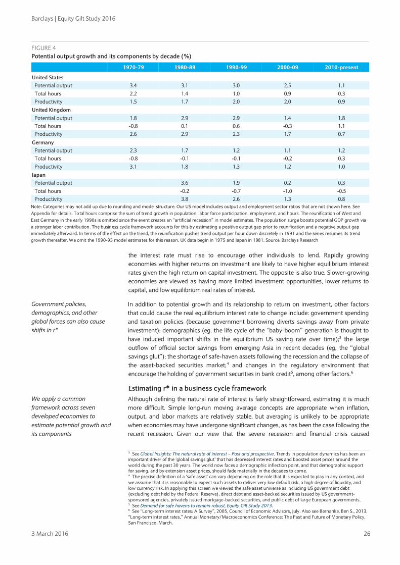
Barclays | Equity Gilt Study 2016
3 March 2016 26
FIGURE 4 Potential output growth and its components by decade (%)
1970-79 1980-89 1990-99 2000-09 2010-present
United States
Potential output 3.4 3.1 3.0 2.5 1.1
Total hours 2.2 1.4 1.0 0.9 0.3 Productivity 1.5 1.7 2.0 2.0 0.9
United Kingdom
Potential output 1.8 2.9 2.9 1.4 1.8 Total hours -0.8 0.1 0.6 -0.3 1.1 Productivity 2.6 2.9 2.3 1.7 0.7
Germany
Potential output 2.3 1.7 1.2 1.1 1.2 Total hours -0.8 -0.1 -0.1 -0.2 0.3
Productivity 3.1 1.8 1.3 1.2 1.0
Japan
Potential output 3.6 1.9 0.2 0.3
Total hours -0.2 -0.7 -1.0 -0.5 Productivity 3.8 2.6 1.3 0.8 Note: Categories may not add up due to rounding and model structure. Our US model includes output and employment sector ratios that are not shown here. See Appendix for details. Total hours comprise the sum of trend growth in population, labor force participation, employment, and hours. The reunification of West and East Germany in the early 1990s is omitted since the event creates an “artificial recession” in model estimates. The population surge boosts potential GDP growth via a stronger labor contribution. The business cycle framework accounts for this by estimating a positive output gap prior to reunification and a negative output gap immediately afterward. In terms of the effect on the trend, the reunification pushes trend output per hour down discretely in 1991 and the series resumes its trend growth thereafter. We omit the 1990-93 model estimates for this reason. UK data begin in 1975 and Japan in 1981. Source: Barclays Research
the interest rate must rise to encourage other individuals to lend. Rapidly growing economies with higher returns on investment are likely to have higher equilibrium interest rates given the high return on capital investment. The opposite is also true. Slower-growing economies are viewed as having more limited investment opportunities, lower returns to capital, and low equilibrium real rates of interest.
In addition to potential growth and its relationship to return on investment, other factors that could cause the real equilibrium interest rate to change include: government spending and taxation policies (because government borrowing diverts savings away from private investment); demographics (eg, the life cycle of the “baby-boom” generation is thought to have induced important shifts in the equilibrium US saving rate over time);3 the large outflow of official sector savings from emerging Asia in recent decades (eg, the “global savings glut”); the shortage of safe-haven assets following the recession and the collapse of the asset-backed securities market;4 and changes in the regulatory environment that encourage the holding of government securities in bank credit5, among other factors.6
Estimating r* in a business cycle framework Although defining the natural rate of interest is fairly straightforward, estimating it is much more difficult. Simple long-run moving average concepts are appropriate when inflation, output, and labor markets are relatively stable, but averaging is unlikely to be appropriate when economies may have undergone significant changes, as has been the case following the recent recession. Given our view that the severe recession and financial crisis caused
3 See Global Insights: The natural rate of interest – Past and prospective. Trends in population dynamics has been an important driver of the ‘global savings glut’ that has depressed interest rates and boosted asset prices around the world during the past 30 years. The world now faces a demographic inflection point, and that demographic support for saving, and by extension asset prices, should fade materially in the decades to come. 4 The precise definition of a ‘safe asset’ can vary depending on the role that it is expected to play in any context, and we assume that it is reasonable to expect such assets to deliver very low default risk, a high degree of liquidity, and low currency risk. In applying this screen we viewed the safe asset universe as including US government debt (excluding debt held by the Federal Reserve), direct debt and asset-backed securities issued by US government-sponsored agencies, privately issued mortgage-backed securities, and public debt of large European governments. 5 See Demand for safe havens to remain robust, Equity Gilt Study 2013. 6 See “Long-term interest rates: A Survey”, 2005, Council of Economic Advisors, July. Also see Bernanke, Ben S., 2013, “Long-term interest rates,” Annual Monetary/Macroeconomics Conference: The Past and Future of Monetary Policy, San Francisco, March.
Government policies, demographics, and other global forces can also cause shifts in r*
We apply a common framework across seven developed economies to estimate potential growth and its components
Barclays | Equity Gilt Study 2016
3 March 2016 27
significant damage to output, the inflation process, and the natural rate of unemployment in developed economies, we use a business cycle framework that estimates the equilibrium real rate of interest from estimates of trend GDP and its cycle. In so doing, we focus implicitly on the link between interest rates and the business cycle. The gap between actual and potential output should contain information about the difference between actual unemployment and its long-run trend and actual interest rates and the natural rate of interest. This is not to say that we ignore the other factors that could cause the natural rate of interest to change. Government policy, demographics, and structural shifts in global capital flows are likely to influence the rate of potential growth and, in turn, alter estimates of the natural rate of interest. We make the simplifying assumption that potential growth and its changes are likely to reflect much of the information needed when forming estimates of r* and understanding the implications for the future conduct of monetary policy.
We apply a business cycle framework to four developed economies – Germany, Japan, the UK, and the US – and break down observed output data into its cyclical and trend components with the goal of jointly estimating potential growth, the natural rate of unemployment, and the real equilibrium interest rate. Although these variables are key inputs in the setting of monetary and fiscal policy and serve as anchors to economic models, they are also unobservable. The framework we apply in this chapter constructs estimates of these key variables using a generalized multivariate unobserved components framework; inputs on working hours, output, employment, population, participation, and the real policy rate are used in a comprehensive framework to generate a decomposition of each variable into trend and cycle components.7,8 The model applied to the US is described in more detail in the appendix, while the approach for the remaining countries is identical to that in The great destruction, Equity Gilt Study 2015.
The post-crisis landscape: Lower potential growth Unsurprisingly, our findings reconfirm the results of our previous analysis that severe recessions intertwined with financial crises are associated with lost output and lower potential growth. Potential growth in many developed economies was already slowing before the recession as workforces aged, the boost to productivity from the technology revolution faded, economies slowly transitioned away from manufacturing toward less-productive services as competitiveness worsened, and trends toward part-time work and more flexible working arrangements weighed on hours. Second, the recession has had a notable effect on potential growth in some developed economies by damaging construction and finance-related activities, distorting the efficient allocation of capital, suppressing rates of capital accumulation, and boosting structural unemployment, among other factors.
Trend growth in the US is estimated to have fallen steadily since 1999 as the benefits of technological progress began to fade and the workforce aged (Figure 4).9 Our findings support the conclusion that the decline in labor force participation since its peak in the early 2000s mainly reflects the ageing and retirement of the baby boom generation as opposed to purely cyclical forces. The post-recession environment has also weighed on productivity growth, likely a consequence of limited resource re-allocation from bubble-inflated sectors and slower rates of business formation as a result of tighter credit and reduced entrepreneurial risk-taking. In addition, the US has been in a gradual transition from a goods-oriented economy to a services economy, the latter of which is associated with more
7 For the US, our approach follows Charles Fleischman and John M. Roberts, 2011, “From many series, one cycle: Improved estimates of the business cycle from a multivariate unobserved components model,” Finance and Economics Discussion Series 2011-46. 8 See Jun Ma and Mark Wohar, “An unobserved components model that yields business and medium-run cycles,” Journal of Money, Credit, and Banking, 45(7), October 2013, for further discussion on the benefits of the unobserved components model. 9 Our US economics team has written frequently about US demographic trends and their contribution to slower potential growth. See Beyond the cycle: Weaker growth, higher unemployment, 15 December 2010 and Dispelling an urban legend: US labor force participation will not stop the unemployment rate decline, 1 March 2012
Our framework jointly estimates potential output, the natural rate of unemployment, and the equilibrium rate of interest
Potential growth slowed markedly heading into the recession… …and the recession further destroyed output and slowed productivity

Barclays | Equity Gilt Study 2016
3 March 2016 28
part-time employment and a shorter average work week.10 Altogether, we estimate that these factors caused US potential GDP growth to slow to 1.1% in the post-recession period. That said, our year-on-year estimates show potential edging up to 1.5% in 2015.
We find similar results for the UK, Germany, and Japan. The slowing of the rate of trend output in the UK is clearly related to slower trend productivity growth. However, growth in hours worked has provided an important offset to the slowing in trend productivity and the “productivity puzzle” looks less pronounced than before.11 A slowing in trend productivity growth is also a feature of Germany and Japan, with output per hour falling to1.0% in the post-crisis period. In contrast to many of its peers, labor force participation has been on a steady upward path. Higher participation, faster growth in trend employment, and stable population growth have been important offsets to weaker productivity. In Japan, demographics, the transition to a more service-based economy, and a decelerating trend in weekly hours explain most of the fall in potential growth heading into the recession. Following the recession, potential GDP remained low as productivity growth fell further.
The natural rate of interest in developed economies has fallen The four economies in our sample have experienced broadly similar outcomes in recent years. Following the recession, observed growth has been modest, but strong enough to boost employment and put persistent downward pressure on unemployment. However, despite the improvement in labor market conditions and narrowing of the output gap, central banks have failed to meet their inflation targets. The fear of runaway inflation early on in the recovery due to significant balance sheet expansion has given way to the expectation of sub-2% inflation for the next decade. Our business cycle framework reconciles this combination of growth, unemployment, and inflation outcomes by slowing trend growth, lowering estimates of long-term unemployment, and reducing the natural rate of interest. Put another way, near-zero interest rates have failed to generate strong activity and/or ignite inflation. The framework suggests the equilibrium interest rate must have fallen and policy was not as stimulative as previously thought. Modest growth and falling unemployment must be consistent with slower potential growth, as illustrated in the previous section.
10 Employment in the goods sector in the US was nearly 40% of total private employment in 1965. The share has fallen to around 15% in recent years, leaving the remainder (85%) in services. Since average weekly hours in the service sector averages about 33 hours, compared to 41 hours for the goods sector, the relative shift into services has caused average weekly hours for the overall US private sector to decline from 39 in 1965 to 34 today. See “U-6 unemployment may not reach normal,” 11 July 2014. 11 The UK “productivity puzzle” has been heavily investigated and several factors put forward to explain the slowdown. A report from the Bank of England points to labor hoarding during the early stages of the recession, reduced investment in physical and tangible capital, and misallocation of resources in low to high productivity sectors. See “The UK productivity puzzle” by Alina Barnett, Sandra Batten, Adrian Chiu, Jeremy Franklin, and Maria Sebastia-Barriel of the Bank of England’s Monetary Analysis Directorate, Bank of England Quarterly Bulletin, 2014 Q2.
Productivity growth has slowed, but growth in total hours has mitigated the effect on potential growth
FIGURE 5 The real equilibrium interest rate in the US
FIGURE 6 Real equilibrium interest rates in the UK, Japan, and Germany
Source: Barclays Research
Source: Barclays Research
0
1
2
3
4
5
6
7
67 71 75 79 83 87 91 95 99 03 07 11 15
% y/y
The real equilibrium rate of interest in the US
-4
-2
0
2
4
6
8
00 01 02 03 04 05 06 07 08 09 10 11 12 13 14 15
%
UK Japan Germany
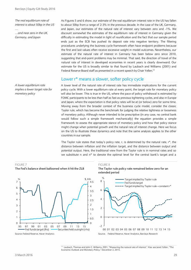
Barclays | Equity Gilt Study 2016
3 March 2016 29
As Figures 5 and 6 show, our estimate of the real equilibrium interest rate in the US has fallen to about 50bp from a range of 2-3% in the previous decade. In the case of the UK, Germany, and Japan, our estimates of the natural rate of interest vary between zero and -1%. We discount somewhat the estimates of the equilibrium rate of interest in Germany given the difficulty in estimating the model in light of reunification and the fact that our sample period ends just as the ECB has pushed its deposit rate into negative territory. The filtering procedures underlying the business cycle framework often have endpoint problems because the first and last values often receive excessive weight in model outcomes. Nevertheless, our estimate of the natural rate of interest in Germany has been below zero since 2010, suggesting that end-point problems may be minimal. That said, the direction of travel of the natural rate of interest in developed economies in recent years is clearly downward. Our estimate for the US is broadly similar to that found by Laubach and Williams (2001) and Federal Reserve Board staff as presented in a recent speech by Chair Yellen.12
Lower r* means a slower, softer policy cycle A lower level of the natural rate of interest rate has immediate implications for the current policy cycle. With a lower equilibrium rate at every point, the target rate for monetary policy will also be lower. This is true in the US, where the pace of policy withdrawal is estimated by FOMC participants to be less than half as fast as previous tightening cycles, and also in Europe and Japan, where the expectation is that policy rates will be at (or below) zero for some time. Moving away from the broader context of the business cycle model, consider the classic Taylor rule, which has become the benchmark for judging the relative tightness or looseness of monetary policy. Although never intended to be prescriptive (in any case, no central bank would follow such a simple framework mechanically) the equation provides a simple framework to assess the appropriate stance of monetary policy and how that policy stance might change when potential growth and the natural rate of interest change. Here we focus on the US to illustrate these dynamics and note that the same analysis applies to the other countries in our sample.
The Taylor rule states that today’s policy rate, r, is determined by the natural rate, r*, the distance between inflation and the inflation target, and the distance between output and potential output. Here, the traditional view from the Taylor rule is in nominal rates and so we substitute n and n* to denote the optimal level for the central bank’s target and a
12 Laubach, Thomas and John C. Williams, 2001, “Measuring the natural rate of interest.” Also see Janet Yellen, “The Economic Outlook and Monetary Policy,” December 2, 2015.
The real equilibrium rate of interest is about 50bp in the US … …and near zero in the UK, Germany, and Japan
A lower equilibrium rate implies a lower target rate for monetary policy
FIGURE 7 The Fed’s balance sheet ballooned when it hit the ZLB
FIGURE 8 The Taylor rule policy rate remained below zero for an extended period
Source: Federal Reserve, Haver Analytics
Source: Federal Reserve, Haver Analytics, Barclays Research
0
0.5
1
1.5
2
2.5
3
3.5
4
4.5
0
1
2
3
4
5
6
7
95 97 99 01 03 05 07 09 11 13 15Fed funds target (lhs) Securities held outright (rhs)
% $, trln
-2
0
2
4
6
8
00 01 02 03 04 05 06 07 08 09 10 11 12 13 14 15
Target implied by Taylor ruleFed funds targetTarget implied by Taylor rule--constant r*
%

Barclays | Equity Gilt Study 2016
3 March 2016 30
nominal version of r*. The Taylor rule is defined:13
𝑛 = 𝑛∗ + 𝜃 ∗ (𝜋 − 𝜋∗ ) + 𝜑 ∗ (𝑦 − 𝑦∗)
If we assume that both inflation and output are close to target and the Fed desires to keep them there, the Fed’s policy rate should be close to r*. Should r* move lower, either permanently or temporarily, the equilibrium policy rate should also be lower. In other words, a lower level of r* and slower potential growth implies that for output and inflation to be balanced the policy rate must also be lower. It also implies that any given level of the policy rate is actually tighter than it would have been a few years ago
How easy is US interest rate policy? The fed funds rate has been mired near zero for a long time, even as growth has remained quite low relative to its historical average. This combination has led some observers to conclude that monetary policy is no longer effective. However, in our framework, what matters for changing growth rates or output is not so much the level of the interest rate but the distance of the policy rate from its natural rate. From an investment perspective, an interest rate is only “low” if it is below the rate of return.
We assume that the natural rate of interest estimated below represents the required rate of return, the price that balances the supply of savings with demand for borrowing. Therefore, monetary policy is not nearly as accommodative as one might think from the level of interest rates. Of course, the level of interest rates does not fully reflect the entire stance of monetary policy, which requires understanding the effects of the expansion of central bank balance sheets. For example, as Figure 7 shows, the Fed pushed its target rate to zero in early 2009 and then launched a $3.5trn asset purchase program.
Nonetheless, and to the extent that we can safely make statements about the stance of interest rate policy separate from balance sheet policy, we use the Taylor rule in Figure 8, applying our estimates of the output gap and r* from our model. For inflation we use the four-quarter change in core PCE inflation. The solid black line shows the nominal policy rate as implied by this Taylor rule. Although a policy rate of zero seems to be very easy monetary policy, we can see from the path of the solid dark line that the zero lower bound is binding on the Fed from early 2009 until early 2014. In an unconstrained world, the Fed would have
13 The weights on the inflation and output gap are unknown parameters and the subject of intense debate among economists. Theory does not provide a tight guide for the relative weight of inflation and activity in conducting monetary policy. Empirical estimates are imprecisely estimated because the two gaps tend to move together. As we discussed in Two minds are not better than one, this lack of guidance drove some of the divergence among FOMC members last year, as those who placed more weight on activity were ready to hike rates and those who placed more weight on inflation were content to hold fast. We do not take a strong stand and simply follow early research to assume that the FOMC’s objective function places equal weight on the inflation and output gaps.
Our estimate of US r* corresponds quite well to actual policy outcomes
FIGURE 9 Core inflation has remained soft, despite low rates
FIGURE 10 Credit growth was slow to rebound, despite low interest rates
Note: The FOMC did not formally adopt an inflation target until 2012. Source: BLS, Haver Analytics, Barclays Research
Source: Federal Reserve, Haver Analytics
0.5
1.0
1.5
2.0
2.5
3.0
00 01 02 03 04 05 06 07 08 09 10 11 12 13 14 15 16
% , y/y
PCE CPI Fed target
-10.0
-5.0
0.0
5.0
10.0
15.0
00 01 02 03 04 05 06 07 08 09 10 11 12 13 14 15 16
%, y/y
Loans and leases at commercial banks

Barclays | Equity Gilt Study 2016
3 March 2016 31
moved the policy rate even lower, which of course is the reason it implemented the asset purchase program. Notably, the implied policy path rose above zero in early 2014. This is consistent with the Fed beginning to taper its asset purchases in December 2013. The movement above zero also explains why Chair Yellen began discussing liftoff in late 2014. With the implied policy rate rising, inaction in monetary policy was actually leading to “looser” policy from the perspective of a simple Taylor rule.
The Taylor rule also sheds light on the policy path in the mid-2000s. Following the 2000 recession, the Fed cut policy aggressively, much faster than the pace implied by the Taylor rule. In 2004, the Fed began its “gradual and measured” rate hike cycle, boosting the policy rate by 25bp at each meeting. One reason for the easy credit conditions and the booming housing market was that the Fed was substantially behind on its rate hike cycle. It was not until late 2005 that the policy became neutral, and it ended up being tight by the time the recession began to emerge. Another reason that Chair Yellen was eager to begin the rate hike cycle was that she believes policy was tightened too slowly in the 2000s.
What if r* in the US did not decline The main reason policy has been able to stay at zero for an extended period without being “too easy” is the substantial decline in r* that has occurred since 2000. The dashed line in Figure 8 shows the interest rate implied by the Taylor rule if r* is held constant at its 2000 level. With this higher level of r*, the policy rate never even falls to zero but rather falls to about the low point of the actual 2000s cycle before rising steadily from 2009. This view of the optimal policy rate likely contributed to some of the very hawkish statements by FOMC members early in the recovery. Using a constant r*, the gradual improvement in the US economy after the recession is evident. As the output gap gradually closes, the Taylor rule implies gradually higher policy rates. Without the decline in r*, the neutral policy rate would currently be close to 4% and monetary policy would be extremely accommodative.
Of course, r* is not truly observable. As a result, the consensus view that r* has fallen since 2000 might be wrong. However, if that were the case, we would expect both inflation and lending to be strong. As Figure 9 shows, when the Fed was slow to normalize rates in the 2000s, both core CPI and PCE inflation moved above 2% and remained at that level until the recession. Since 2008, inflation has remained mired stubbornly below the Fed’s target rate. Even with the added expansion of the balance sheet, the Fed has managed only to just support inflation, a very strong indication that policy has not been excessively loose.
Loose policy should also lead to high credit growth. In the 2000s, for which the Taylor rule indicates loose monetary policy, total bank lending rose at a steady 12% (Figure 10). In the current recovery, with our Taylor rule showing policy as still relatively tight, loan growth is very
Low inflation and slow loan growth in the US until 2014 are consistent with a drop in r*
FIGURE 11 Global inflation remains below central bank targets
FIGURE 12 Outside of Japan, lending growth is below pre-crisis levels
Note: Core inflation. Japanese inflation adjusted for effects of 2014 VAT increase. Source: ONS, ECB, MIC, Haver Analytics, Barclays Research
Note: Nominal bank lending growth. Source: BoE, Eurostat, BoJ, Haver Analytics
-2
-1
0
1
2
3
4
97 99 01 03 05 07 09 11 13 15
%, y/y
UK EA Japan
-10
-5
0
5
10
15
20
25
30
35
00 02 04 06 08 10 12 14 16
%, y/y
UK EA Japan

Barclays | Equity Gilt Study 2016
3 March 2016 32
low or negative. It has become consistently positive as policy has moved toward neutral and, in early 2014, as the Taylor rule rate moved above the actual policy rate, loan growth began to accelerate. Because the Taylor rule does not take loan growth into account, the acceleration in lending serves as partial independent confirmation of the relative stance of monetary policy.
A similar story can be found in the inflation and bank lending data of Europe, the UK, and Japan. In Japan, core inflation was mired below zero for much of the past decade, but inflation in Europe and the UK remained near central bank targets until the recession (Figure 11). Since 2011, inflation in these economies has drifted lower while, in Japan, unconventional balance sheet policies were successful at pushing inflation (adjusted for the effects of the 2014 VAT hike) above zero. The fact that inflation remains at or somewhat below targets is indicative of less stimulative monetary policy; a result that would occur if the equilibrium policy rate had fallen. Loan growth has also been virtually flat in these countries since 2009 (Figure 12), further indicating that interest rate policy was not sufficiently loose.
Finally, another way of thinking about the level of monetary policy accommodation is through actual costs of capital. The real cost of borrowing for US firms has declined substantially since the early 1980s (Figure 13). The blue lines in the figure indicate that corporate borrowing rates stepped down after the last recession, consistent with our step down in the r* and the decline in the real fed funds rate. If the decline in corporate borrowing owed to accommodative policy rather than to a decline in r*, we would expect a surge in capital investment.14 Investment as a percentage of GDP (Figure 14) recovered quickly after the recession but did not boom and remains just below its pre-recession average. Altogether, we find the behavior of realized inflation, loan growth, cost of capital, and investment following the recession consistent with our estimates of a lower natural rate of interest.
With low r*, the zero lower bound is omnipresent If current beliefs about the likely evolution of the natural rate of interest prove true, actual interest rates should remain much lower than past averages over the next decade. Furthermore, because our view on low interest rates is driven, in part, by estimates of lower potential growth, the possibility that recessions are likely to be more common than in the past may cause the lower bound to be reached more frequently. In Japan, average growth dropped from an average of 4.5% in the 1980s to 0.7% over the past 20 years. Over that period, GDP growth turned negative 17 times (on five occasions the decline was sufficient
14 Recall, a fall in r* also reflects a fall in the marginal product of capital (MPK) or the return firms receive for investing in an extra unit of capital. If the cost of borrowing is below the MPK, firms can boost profit by borrowing to expand.
FIGURE 13 Real US corporate borrowing rates stepped down after the last recession
FIGURE 14 US equipment investment recovered after the recession but did not boom
Note: US Baa corporate bond rate deflated by y/y core CPI inflation. Expansion average is the average rate 6 months after start of expansion to next recession. Source: Moody’s, Haver Analytics, Barclays Research
Source: BEA, Haver Analytics, Barclays Research
Soft lending and inflation data in the UK, Germany, and Japan are also consistent with a low natural rate of interest
The real cost of borrowing for US firms has tracked the slowdown in potential GDP
-5
0
5
10
15
60 64 68 72 76 80 84 88 92 96 00 04 08 12 16
%
RecessionReal corporate bond rateCorporate expansion average
4.0
4.5
5.0
5.5
6.0
6.5
03 04 05 06 07 08 09 10 11 12 13 14 15
% of GDP
Equipment investment
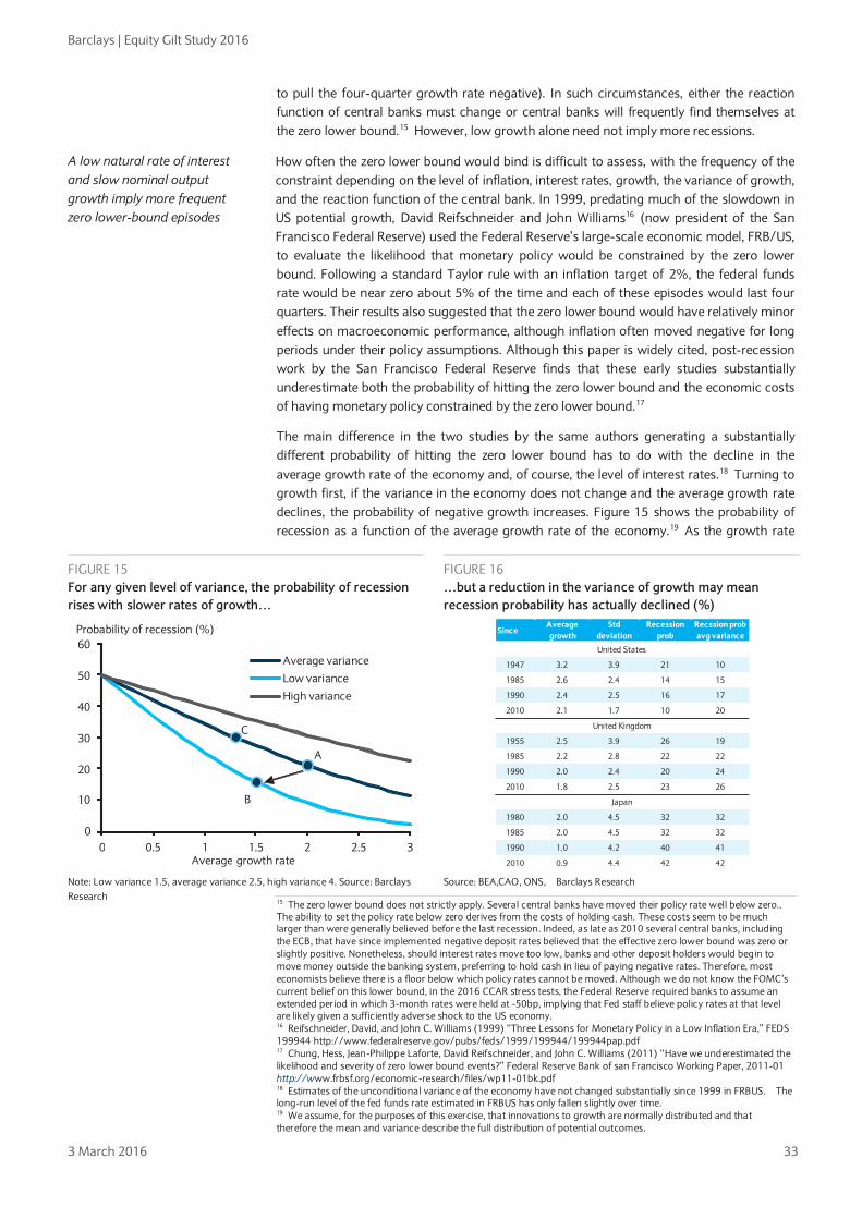
Barclays | Equity Gilt Study 2016
3 March 2016 33
to pull the four-quarter growth rate negative). In such circumstances, either the reaction function of central banks must change or central banks will frequently find themselves at the zero lower bound.15 However, low growth alone need not imply more recessions.
How often the zero lower bound would bind is difficult to assess, with the frequency of the constraint depending on the level of inflation, interest rates, growth, the variance of growth, and the reaction function of the central bank. In 1999, predating much of the slowdown in US potential growth, David Reifschneider and John Williams16 (now president of the San Francisco Federal Reserve) used the Federal Reserve’s large-scale economic model, FRB/US, to evaluate the likelihood that monetary policy would be constrained by the zero lower bound. Following a standard Taylor rule with an inflation target of 2%, the federal funds rate would be near zero about 5% of the time and each of these episodes would last four quarters. Their results also suggested that the zero lower bound would have relatively minor effects on macroeconomic performance, although inflation often moved negative for long periods under their policy assumptions. Although this paper is widely cited, post-recession work by the San Francisco Federal Reserve finds that these early studies substantially underestimate both the probability of hitting the zero lower bound and the economic costs of having monetary policy constrained by the zero lower bound.17
The main difference in the two studies by the same authors generating a substantially different probability of hitting the zero lower bound has to do with the decline in the average growth rate of the economy and, of course, the level of interest rates.18 Turning to growth first, if the variance in the economy does not change and the average growth rate declines, the probability of negative growth increases. Figure 15 shows the probability of recession as a function of the average growth rate of the economy.19 As the growth rate
15 The zero lower bound does not strictly apply. Several central banks have moved their policy rate well below zero.. The ability to set the policy rate below zero derives from the costs of holding cash. These costs seem to be much larger than were generally believed before the last recession. Indeed, as late as 2010 several central banks, including the ECB, that have since implemented negative deposit rates believed that the effective zero lower bound was zero or slightly positive. Nonetheless, should interest rates move too low, banks and other deposit holders would begin to move money outside the banking system, preferring to hold cash in lieu of paying negative rates. Therefore, most economists believe there is a floor below which policy rates cannot be moved. Although we do not know the FOMC’s current belief on this lower bound, in the 2016 CCAR stress tests, the Federal Reserve required banks to assume an extended period in which 3-month rates were held at -50bp, implying that Fed staff believe policy rates at that level are likely given a sufficiently adverse shock to the US economy. 16 Reifschneider, David, and John C. Williams (1999) “Three Lessons for Monetary Policy in a Low Inflation Era,” FEDS 199944 http://www.federalreserve.gov/pubs/feds/1999/199944/199944pap.pdf 17 Chung, Hess, Jean-Philippe Laforte, David Reifschneider, and John C. Williams (2011) “Have we underestimated the likelihood and severity of zero lower bound events?” Federal Reserve Bank of san Francisco Working Paper, 2011-01 http://www.frbsf.org/economic-research/files/wp11-01bk.pdf 18 Estimates of the unconditional variance of the economy have not changed substantially since 1999 in FRBUS. The long-run level of the fed funds rate estimated in FRBUS has only fallen slightly over time. 19 We assume, for the purposes of this exercise, that innovations to growth are normally distributed and that therefore the mean and variance describe the full distribution of potential outcomes.
FIGURE 15 For any given level of variance, the probability of recession rises with slower rates of growth…
FIGURE 16 …but a reduction in the variance of growth may mean recession probability has actually declined (%)
Note: Low variance 1.5, average variance 2.5, high variance 4. Source: Barclays Research
Source: BEA,CAO, ONS, Barclays Research
A low natural rate of interest and slow nominal output growth imply more frequent zero lower-bound episodes
SinceAverage growth
Std deviation
Recession prob
Recssion prob avg variance
1947 3.2 3.9 21 10
1985 2.6 2.4 14 15
1990 2.4 2.5 16 17
2010 2.1 1.7 10 20
1955 2.5 3.9 26 19
1985 2.2 2.8 22 22
1990 2.0 2.4 20 24
2010 1.8 2.5 23 26
1980 2.0 4.5 32 32
1985 2.0 4.5 32 32
1990 1.0 4.2 40 41
2010 0.9 4.4 42 42
United States
United Kingdom
Japan
0
10
20
30
40
50
60
0 0.5 1 1.5 2 2.5 3
Average variance Low variance High variance
Average growth rate
Probability of recession (%)
A
B
C

Barclays | Equity Gilt Study 2016
3 March 2016 34
falls toward zero, the probability of recession in any year rises to 50% (think of the case of Japan). At zero growth, assuming positive and negative shocks are symmetric, the probability of negative growth in any period is 50%, independent of the variance. Effectively, Reifschnieder and Williams consider the case of an economy sliding along one of the variance curves as growth slows (say from point A to point C).
However, lower growth does not necessarily lead to a higher probability of recession. Low- variance economies have a lower probability of recession than those with high variance. As a result, if an economy undergoes a sufficiently large reduction in variance that coincides with the decrease in average growth rate, the probability of recession can decline. For example, an economy that moved from average variance and 2% growth (point A) moved to low variance and 1.5% growth (point B), the probability of recession would fall from around 20% to 15%. Falling growth and variance tends to be the US experience.
This story fits the US economy, where the average growth rate and variance output have declined over time. Figure 16 give the results of this exercise using actual GDP data. Row 1 of the table shows that the average growth rate of the economy since 1947 was 3.2% and the standard deviation of output over the same period was 3.9%. This implies an unconditional recession probability of 21%. Of course, this high frequency of recession owed to the very volatile years immediately after WWII. From 1985 to the present, a period that includes the Great Moderation, the average growth rate of the economy fell to 2.6% and the standard deviation of output growth fell from 3.9 to 2.4. Because the volatility of output also fell, the probability of recession declined from 21% to 14%. Likewise, since 2010, the average growth rate of the economy has declined further, to 2.1%, but the volatility fell even further, implying that the unconditional probability of recession declined to about 10%.
The sample since 2010 is quite short and we do not expect volatility to stay repressed for an extended period, but the data are nevertheless instructive. Should the variance of output rise, the probability of recession would increase as well. Although we see much of the decline in variance as structural, we believe the standard deviation in the last row of the table somewhat overstates the decline. If, as shown in the last column of the table, we compute recession probability using the average standard deviation since 1990, the probability of recession rises to 20%. We would estimate that the unconditional probability of recession lies somewhere between 10 and 20%, or not substantially different from previous decades.
However, even if the probability of a recession is much lower, the probability of hitting the ZLB remains elevated. Because r* is lower and the FOMC’s inflation target is unchanged, the Fed has less room to lower its policy rate when recessions occur. Since the Fed has typically cut the fed funds rate by more than 4pp during recessions, the zero lower bound is very likely to
FIGURE 17 The share of services value added in US GDP has risen…
FIGURE 18 …as has the share of US services employment
Source: BEA, Haver Analytics Source: BLS, Haver Analytics
However, a shift toward service sector value added may mean growth is more stable at lower rates; slow growth need not coincide with a higher frequency of recessions
0.2
0.3
0.4
0.5
0.6
0.7
0.8
49 54 59 64 69 74 79 84 89 94 99 04 09 14
US services US goods
Share of value added
0.5
0.6
0.7
0.8
0.9
50 55 60 65 70 75 80 85 90 95 00 05 10 15
Services share of employment
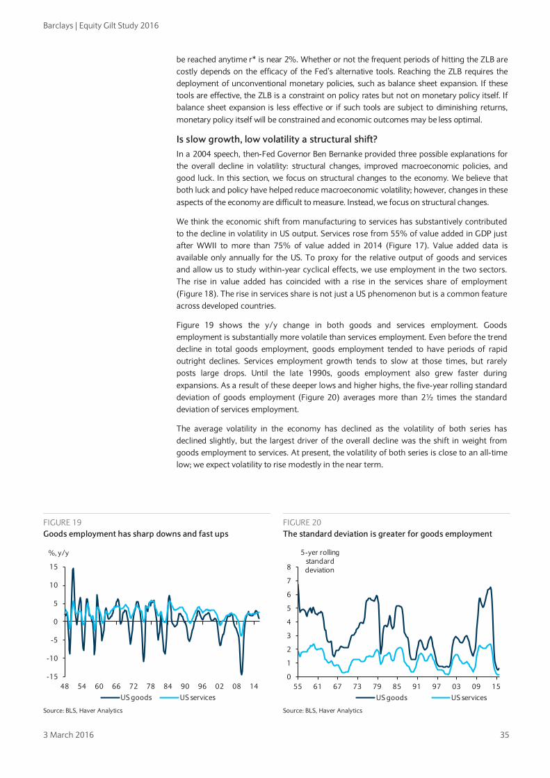
Barclays | Equity Gilt Study 2016
3 March 2016 35
be reached anytime r* is near 2%. Whether or not the frequent periods of hitting the ZLB are costly depends on the efficacy of the Fed’s alternative tools. Reaching the ZLB requires the deployment of unconventional monetary policies, such as balance sheet expansion. If these tools are effective, the ZLB is a constraint on policy rates but not on monetary policy itself. If balance sheet expansion is less effective or if such tools are subject to diminishing returns, monetary policy itself will be constrained and economic outcomes may be less optimal.
Is slow growth, low volatility a structural shift? In a 2004 speech, then-Fed Governor Ben Bernanke provided three possible explanations for the overall decline in volatility: structural changes, improved macroeconomic policies, and good luck. In this section, we focus on structural changes to the economy. We believe that both luck and policy have helped reduce macroeconomic volatility; however, changes in these aspects of the economy are difficult to measure. Instead, we focus on structural changes.
We think the economic shift from manufacturing to services has substantively contributed to the decline in volatility in US output. Services rose from 55% of value added in GDP just after WWII to more than 75% of value added in 2014 (Figure 17). Value added data is available only annually for the US. To proxy for the relative output of goods and services and allow us to study within-year cyclical effects, we use employment in the two sectors. The rise in value added has coincided with a rise in the services share of employment (Figure 18). The rise in services share is not just a US phenomenon but is a common feature across developed countries.
Figure 19 shows the y/y change in both goods and services employment. Goods employment is substantially more volatile than services employment. Even before the trend decline in total goods employment, goods employment tended to have periods of rapid outright declines. Services employment growth tends to slow at those times, but rarely posts large drops. Until the late 1990s, goods employment also grew faster during expansions. As a result of these deeper lows and higher highs, the five-year rolling standard deviation of goods employment (Figure 20) averages more than 2½ times the standard deviation of services employment.
The average volatility in the economy has declined as the volatility of both series has declined slightly, but the largest driver of the overall decline was the shift in weight from goods employment to services. At present, the volatility of both series is close to an all-time low; we expect volatility to rise modestly in the near term.
FIGURE 19 Goods employment has sharp downs and fast ups
FIGURE 20 The standard deviation is greater for goods employment
Source: BLS, Haver Analytics Source: BLS, Haver Analytics
-15
-10
-5
0
5
10
15
48 54 60 66 72 78 84 90 96 02 08 14
%, y/y
US goods US services
0
1
2
3
4
5
6
7
8
55 61 67 73 79 85 91 97 03 09 15
5-yer rolling standard deviation
US goods US services
Barclays | Equity Gilt Study 2016
3 March 2016 36
Appendix: US business cycle framework Potential output, the output gap, the natural rate of unemployment, and the natural rate of interest are key variables in understanding the setting of monetary and fiscal policy, and serve as anchors to economic models. However, they are unobservable and statistical methods are needed to break down movements in observable variables into trend and cycle estimates. The framework applied to the US in this analysis constructs estimates of the unobserved variables above using a multivariate approach; inputs on working hours, output, employment, unemployment, and the labor force are used in a multivariate framework to break down potential output growth into its components.20 The framework is similar in structure to that in “The great destruction,” Equity Gilt Study 2015, but we have altered the specifications of some variables and added terms to estimate the real equilibrium rate of interest.
There are several advantages to a multivariate approach. Academic research has shown that it improves the accuracy of cycle estimates and using a single system means the framework uniformly accounts for trade-offs between alternative signals.21 Each measure of economic activity and labor markets is represented as the sum of cyclical and trend components, with an idiosyncratic residual. The cyclical component (cyc) is assumed to be common across all of the inputs with contemporaneous and, in some cases, lagged effects, while each variable is permitted to have its own unique trend. In addition, we assume a partial-adjustment process that allows for rigidities or other adjustment costs that prevent variables from fully adjusting in the current period in response to cyclical shocks.
The US multivariate framework Our US framework includes the following variables: real gross domestic product (GDP), real gross domestic income (GDI), real nonfarm business output (NFBP), real nonfarm business income (NFBI), nonfarm business employment (ENFB), the work week (WW), the labor force participation rate (LR), the employment rate (ER), and core CPI inflation (CPI). The use of variables from both the product side and income side should improve our ability to estimate the common cycle. All variables are in log terms and the civilian working-age population is subtracted from real gross domestic product, real gross domestic income, real nonfarm business output, real nonfarm business income, and nonfarm business employment.
The GDP, GDI, NFBP, and NFBI equations are given by
𝐺𝐷𝑃𝑡 = 𝐺𝐷𝑂𝑡∗ + 𝑐𝑦𝑐𝑡 + 𝑢𝑖𝑡
𝐺𝐷𝐼𝑡 = 𝐺𝐷𝑂𝑡∗ + 𝑐𝑦𝑐𝑡 + 𝑢2𝑡
𝑁𝐹𝐵𝑃𝑡 = 𝑁𝐹𝐵𝑂𝑡∗ + 𝛾10𝑐𝑦𝑐𝑡 + 𝑢3𝑡
𝑁𝐹𝐵𝐼𝑡 = 𝑁𝐹𝐵𝑂𝑡∗ + 𝛾10𝑐𝑦𝑐𝑡 + 𝑢4𝑡
where GDO* represents the common trend component of GDP and GDI (eg, potential output) and NFBO* the common trend between NFBP and NFBI.22,23 The framework assumes the residuals are measurement errors that can be broken down into the sum of a common component and idiosyncratic components. Potential output and nonfarm
20 Our approach follows Charles Fleischman and John M. Roberts, 2011, “From many series, one cycle: Improved estimates of the business cycle from a multivariate unobserved components model,” Finance and Economics Discussion Series 2011-46; and Jun Ma and Mark Wohar, “An unobserved components model that yields business and medium run cycles,” August 2012. 21 Arabinda Basistha and Richard Startz, 2008, “Measuring the NAIRU with reduced uncertainty: A multiple-indicator common-cycle approach,” Review of Economics and Statistics, 90, 805-11. Also see James H. Stock and Mark W. Watson, 1989, “New indices of coincident and leading economic indicators,” NBER Macroeconomics Annual 1989, Oliver Blanchard and Stanley Fischer, eds., 351-394. 22 The cycle is assumed to be a stationary AR(2) process equal to 𝑐𝑦𝑐𝑡 = 𝜌1𝑐𝑦𝑐𝑡−1 + 𝜌2𝑐𝑦𝑐𝑡−2 + 𝜔𝑡.Typically 𝜌1 > 0 and 𝜌2 < 0 which implies the cycle is hump-shaped in response to a shock. The sum of the coefficients is assumed to be close to 1, but less than 1, meaning the business cycle is persistent. 23 Since NFBO is not the same as GDO (since it exclude the farm and public sectors), 𝛾=1 cannot be assumed for a contemporaneous, normalized cycle. We estimate 𝛾 = 𝛾10 and assume it is the same across both variables with the prior that nonfarm business output likely has larger amplitude than GDO since the latter includes the public sector.
Barclays | Equity Gilt Study 2016
3 March 2016 37
business output can be further broken down into component parts according to 𝐺𝐷𝑂𝑡∗ = 𝑁𝐹𝐵𝑂𝑡∗ + 𝑂𝑆𝑅𝑡∗
𝑁𝐹𝐵𝑂𝑡∗ = 𝐻𝑁𝐹𝐵𝑡∗ + 𝑂𝑃𝐻𝑡∗
𝐻𝑁𝐹𝐵𝑡∗ = 𝐸𝑁𝐹𝐵𝑡∗ + 𝑊𝑊𝑡∗
𝐸𝑁𝐹𝐵𝑡∗ = 𝐸𝐶𝑃𝑆𝑡∗ + 𝐸𝑆𝑅𝑡∗
𝐸𝐶𝑃𝑆𝑡∗ = 𝐸𝑅𝑡∗ + 𝐿𝑃𝑡∗
where OSR* is the output sector ratio between gross domestic output and nonfarm business output, HNFB* is the trend of total working hours, OPH* is the trend of output per hour or productivity, ENFB* is the trend in total employment, WW* is the trend of average working hours, ER* is the employment rate, and LP* is the labor force participation rate. ECPS* is the trend in employment from the current population survey and ESR* is the employment sector ratio between total employment and the current population survey.
The observed data on employment, the work week, the employment rate, and participation are broken down into the sum of a trend, cycle, and partial adjustment term according to
𝐸𝑁𝐹𝐵𝑡 = 𝐸𝑁𝐹𝐵𝑡∗ + 𝛾20𝑐𝑦𝑐𝑡 + 𝜑2(𝐸𝑁𝐹𝐵𝑡−1 − 𝐸𝑁𝐹𝐵𝑡−1∗ ) + 𝑢5𝑡
𝑊𝑊𝑡 = 𝑊𝑊𝑡∗ + 𝛾30𝑐𝑦𝑐𝑡 + 𝛾31(𝑐𝑦𝑐𝑡 − 𝑐𝑦𝑐𝑡−1) + 𝜑3(𝑊𝑊𝑡−1 −𝑊𝑊𝑡−1
∗ ) + 𝑢6𝑡
𝐸𝑅𝑡 = 𝐸𝑅𝑡∗ + 𝛾40𝑐𝑦𝑐𝑡 + 𝜑4(𝐸𝑅𝑡−1 − 𝐸𝑅𝑡−1∗ ) + 𝑢7𝑡
𝐿𝐹𝑅𝑃𝑡 = 𝐿𝐹𝑃𝑅𝑡∗ + 𝛾50𝑐𝑦𝑐𝑡 + 𝜑5(𝐿𝐹𝑃𝑅𝑡−1 − 𝐿𝐹𝑃𝑅𝑡−1∗ ) + 𝑢8𝑡
where the framework allows for some deviation between shocks to output and the response of employment hours and labor force participation. The idea behind the partial adjustment formulation is that the observed variable may be related to its trend, but there may also be inertia in the system such that the observed value is a compromise between its value in the previous period and the value justified by the current trend. The coefficient 𝜑 describes the speed of adjustment between periods where a value of 0 indicates no adjustment and a value of 1 indicates full adjustment from the current period. The rationale for this specification is similar to the one we used to justify including lags of the cycle; adjustment costs may mean firms find it costly to adjust the factors of production so that changes in labor market activity may lag changes in output. If present, these adjustment costs could preclude full adjustment from one period to the next.
Finally, the Phillips curve is given by
𝐷𝑃𝐶𝑋𝐹𝐸𝑡 = 𝛼1𝐷𝑃𝐶𝑋𝐹𝐸𝑡−1 + (1 − 𝛼1)𝑃𝑇𝑅𝑡 + 𝛽11(𝐿)𝑑𝑟𝑝𝑒𝑡−1 + 𝛽12(𝐿)𝑑85𝑡𝑑𝑟𝑝𝑒𝑡−1
+𝛽2(𝐿)𝑑𝑟𝑝𝑖𝑡 + 𝜃(𝛾20𝑐𝑦𝑐𝑡 + 𝛾21𝑐𝑦𝑐𝑡−1 + 𝛾22𝑐𝑦𝑐𝑡−2) + 𝑢9𝑡
where 𝐷𝑃𝐶𝑋𝐹𝐸 is the change in core PCE inflation, 𝑃𝑇𝑅 is a measure of long-run inflation expectations, 𝑑𝑟𝑝𝑒 is the relative change in consumer energy prices, 𝑑𝑟𝑝𝑖 is the change in the relative price of imports, 𝑑85 is a dummy from 1985 to the present to account for rising share of the import ratio in consumer spending, and (L) represents lagged values. Like Roberts (2014) we constrain the sum of the coefficients on lagged inflation and 𝑃𝑇𝑅 to be equal to one. The inflation equation also assumes cyclical deviations in output from its trend affect inflation.
Natural rate of interest The specification for the natural rate of interest is similar to that in Laubach and Williams (2001)24. Since the Federal Reserve and, indeed, nearly all major central banks use a short-term interest rate as the primary tool of policy, it is useful to estimate the natural rate of
24 Laubach, Thomas and John C. Williams, 2001, “Measuring the natural rate of interest.”

Barclays | Equity Gilt Study 2016
3 March 2016 38
interest simultaneously with estimates of potential output, trend employment rate, and inflation. The advantage of this specification is that it provides a useful metric to understand the long-run stance of monetary policy. Its chief weakness is that it abstracts from many other factors that are thought to cause variations in the natural rate of interest, including, but not limited to, demographics, the “global saving glut”, the safe-asset shortage, changes in the regulatory environment, inflation risk and the term premium, deleveraging, secular stagnation, and tail risks and fundamental uncertainty.25
Identification of the trend real rate of interest (R*) is done by relating the output gap, or estimate of the cycle, to two lags of the real interest rate gap according to
𝑐𝑦𝑐𝑡 = 𝜌1𝑐𝑦𝑐𝑡−1 + 𝜌2𝑐𝑦𝑐𝑡−2 + 𝜑6(𝑅𝑡−1 − 𝑅𝑡−1∗ ) + 𝜑6(𝑅𝑡−2 − 𝑅𝑡−2∗ ) + 𝜂𝑡
with the imposed restriction that the coefficients on the two lags of the real rate gap are the same (Laubach and Williams (2001) makes a similar assumption). Because the output gap in most empirical studies is characterized as an AR(2) process, we specify two lags of the interest rate gap. To construct an estimate of the real policy rate (R), we subtract the measure of long-run inflation expectations (PTR) from the effective federal funds rate. The model is estimated using quarterly data from Q1 1967Q1 to Q3 2015 using maximum-likelihood techniques in the state-space model estimation framework in Eviews.
25 See “Long-term interest rates: A Survey”, 2005, Council of Economic Advisors, July. Also see Bernanke, Ben S., 2013, “Long-term interest rates,” Annual Monetary/Macroeconomics Conference: The Past and Future of Monetary Policy, San Francisco, March.

Barclays | Equity Gilt Study 2016
3 March 2016 39
CHAPTER 3
Negative ascent: Life amid negative nominal interest rates • Negative nominal interest rates are more than just a passing monetary fad. In a
world with persistent and pervasive negative real risk-free interest rates and "Missingflation", they may be the only tool available to central banks that can stimulate moribund economies.
• Three key frictions differentiate negative nominal rates from positive rates and will challenge policymakers: 1) currency as an alternative; 2) "money illusion" – an aversion to nominal losses – and its politics; and 3) long-term nominal commitments of pensions and insurers. While the former two are better known, the latter may be more determinative of the "negative lower bound" in some economies.
• Uncertainty over the negative lower bound, the above-mentioned frictions, and reduced wealth effects due to money illusion may dampen the impact of interest rate cuts below zero relative to similar moves in positive territory.
• But well designed tiering of negative rates on bank reserves can work around some of these frictions and provide powerful new tools for central banks to stimulate lending to the non-financial sector.
In a frictionless world, there would be no difference between negative nominal interest rates and positive interest rates; only the sign would change. Negative nominal rates (NNR) would be just another number. But the world is not frictionless. The existence of nominal rigidities – including “money illusion”, currency as an alternative, and long-lived nominal liabilities – means that, in practice, the impact on the economy and asset prices of NNR may differ greatly from the effect of positive interest rates.
Yet, negative nominal rates appear to be ascendant. Pervasive low or negative real interest rates, “Missingflation”, and the unclear success of other “unconventional” monetary policies to address declining inflation have led several developed economy central banks to experiment with NNR as a policy tool. So far – in chronological order – the Danmarks Nationalbank (DNB), the European Central Bank (ECB), the Swedish Riksbank, the Swiss National Bank (SNB)1, and the Bank of Japan (BoJ) have instituted some form of NNR, while the Bank of England (BoE), Bank of Canada (BoC) and Federal Reserve (Fed) all have publicly discussed NNR’s potential as a policy tool should conditions merit their use.
We examine the implications of a world of NNR. We start with an exploration of why central banks are increasingly turning from other unconventional policies to NNR. Next, we look at the nominal frictions that might impair the efficacy of NNR – the existence of notes and coins, the politics of money illusion, legacy long-term nominal liabilities, and the transactions demand for money – and how those may determine the “negative lower bound” (NLB) for interest rates. Finally, we turn to what NNR and those frictions mean for monetary policy, fiscal sustainability, banking, asset management, asset pricing, and foreign exchange.
1 Here we refer to this economic cycle. The SNB was the first to experiment with NNR in the 1970s.
Marvin Barth +44 (0)20 3134 3355 [email protected] Barclays, UK Zoso Davies +44 (0)20 7773 5815 [email protected]
Barclays, UK Antonio Garcia Pascual +44 (0)20 3134 6225 [email protected] Barclays, UK Christian Keller
+44 (0)20 7773 2031 [email protected] Barclays, UK Giuseppe Maraffino +44 (0)20 3134 9938 giuseppe.maraffino@ barclays.com Barclays, UK

Barclays | Equity Gilt Study 2016
3 March 2016 40
The economics of negative nominal rates
The policy case for negative nominal rates The turn to NNR by a handful of central banks has its roots in recent extraordinary economic circumstances. Most developed economies are operating below capacity, with persistently below-target and falling core inflation (Figure 1, Chapter 1: The fight to bring back inflation). This situation has endured despite zero or near-zero nominal policy rates and a variety of unorthodox policy measures over the past eight years. With 5y risk-free real interest rates mired at or below zero since the global financial crisis (GFC) and “Missingflation” threatening to raise them, despite historically low nominal interest rates, central banks need a new weapon in their fight against disinflation and stagnation (Figure 2).
In “normal” circumstances, central banks would cut nominal short-term interest rates, which, in the presence of sticky prices, would lower real interest rates to make capital investment more attractive and stimulate economic activity to absorb excess capacity and put upward pressure on inflation. But the GFC presented central banks with an unusually difficult situation.
Because of the unusually large contraction in output and years of pre-GFC overinvestment, the marginal product of capital (MPK) of available investment projects fell for even long-horizon projects. At the same time, an overhang of excessive leverage, combined with the severe adverse shock to real incomes and wealth, pushed risk premia higher. Even with nominal policy rates cut to zero, central banks could not get real borrowing costs low enough to make capital investment attractive (Figure 3; for simplicity, Figures 3, 4 and 8 assume zero inflation, so nominal and real rates are equivalent).
Unconventional monetary policies: A mixed record To address this problem, central banks have unveiled an inventive array of unconventional monetary policies, including verbal forward guidance, quantitative easing (QE) and funding for lending schemes (FLS). Forward guidance aimed to reduce policy rate expectations and to decrease term premia and risk premia by diminishing uncertainty about future economic outcomes. However, to be truly effective, forward guidance required a credible commitment to keep rates low even if the economy improved.2
2 The academic literature distinguishes between “Delphic” forward guidance that is based on forecasts, but reversible, and “Odyssian” forward guidance that includes a commitment not to change policy even if economic circumstances change. Since no central bank can credibly commit not to change course if the economy improves, a better example of Odyssian forward guidance is QE, as it is less easily reversible and is an effective commitment to lower for longer policy rates. See Campbell, Evans, Fisher, and Justiniano, 2012, “Macroeconomic Effects of Federal Reserve Forward Guidance,” Brookings Papers on Economic Activity, vol. 44(1), pp. 1-80.
FIGURE 1 G10 core-inflation deviation from target versus output gaps
FIGURE 2 Global real interest rates versus sovereign risk premium
Source: Haver Analytics, Barclays Research
Source: Bloomberg, IMF, Barclays Research
Negative rates are consequence of ‘missingflation’…
…and the need to push real rates lower
-3
-2
-1
0
1
-4 -2 0 2 4 6
Inflation vs target (%)
Output gap (%pts of GDP)
2015 2007
-4
-2
0
2
4
6
8
10
12
14
0 100 200 300 400 500
Real 5y yield (%)
CDS (bps)Jan'16 Jan'07 GDP-wtd average (2002-16)
20092012
2013
2016
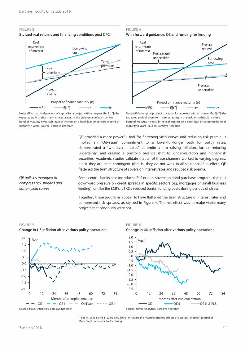
Barclays | Equity Gilt Study 2016
3 March 2016 41
QE provided a more powerful tool for flattening yield curves and reducing risk premia. It implied an “Odyssian” commitment to a lower-for-longer path for policy rates, demonstrated a “whatever it takes” commitment to raising inflation, further reducing uncertainty, and created a portfolio balance shift to longer-duration and higher-risk securities. Academic studies validate that all of these channels worked to varying degrees, albeit they are state contingent (that is, they do not work in all situations).3 In effect, QE flattened the term structure of sovereign interest rates and reduced risk premia.
Some central banks also introduced FLS or non-sovereign bond purchase programs that put downward pressure on credit spreads in specific sectors (eg, mortgages or small business lending), or, like the ECB’s, LTROs reduced banks’ funding costs during periods of stress.
Together, these programs appear to have flattened the term structure of interest rates and compressed risk spreads, as stylized in Figure 4. The net effect was to make viable many projects that previously were not.
3 See M. Weale and T. Wieladek, 2016 “What are the macroeconomic effects of asset purchases?” Journal of Monetary Economics, forthcoming.
FIGURE 5 Change in US inflation after various policy operations
FIGURE 6 Change in UK inflation after various policy operations
Source: Haver Analytics, Barclays Research
Source: Haver Analytics, Barclays Research
FIGURE 3 Stylized real returns and financing conditions post GFC
FIGURE 4 With forward guidance, QE and funding for lending
Note: MPK: marginal product of capital for a project with an n-year life; E[r⁰]: the expected path of short-term interest rates; rⁿ: the yield on a default risk-free bond of maturity n years; bⁿ: rate of interest on a bank loan or corporate bond of maturity n years. Source: Barclays Research
Note: MPK: marginal product of capital for a project with an n-year life; E[r⁰]: the expected path of short-term interest rates; rⁿ: the yield on a default risk-free bond of maturity n years; bⁿ: rate of interest on a bank loan or corporate bond of maturity n years. Source: Barclays Research
QE policies managed to compress risk spreads and flatten yield curves
-2.0
-1.5
-1.0
-0.5
0.0
0.5
1.0
1.5
2.0
0 12 24 36 48 60 72 84
%pa
Months after implementationQE I QE II OpTwist QE III
-3.5-3.0-2.5-2.0-1.5-1.0-0.50.00.51.01.52.0
0 12 24 36 48 60 72 84
%pa
Months after implementationQE I QE II QE III & FLS
Real return/rate of interest
Project or finance maturity (n)
MPK E[r⁰] rⁿ bⁿ
Risk premium
Term premium
Borrowingcost
Project returns
Real return/rate of interest
Project or finance maturity (n)
MPK E[r⁰] rⁿ bⁿ
Projects not undertaken
Project returns
Borrowingcost
Projectsundertaken
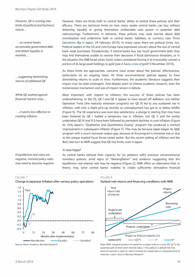
Barclays | Equity Gilt Study 2016
3 March 2016 42
However, there are limits both to central banks’ ability to extend these policies and their efficacy. There are technical limits on how many assets central banks can buy without distorting liquidity or giving themselves undesirable veto power in potential debt restructurings. Furthermore, in extremis, these policies may raise worries about debt monetization and undermine faith in central banks’ liabilities, ie, currency (see Three Questions: Big in Japan, 24 February 2014). In many cases there are political limits, too. Political leaders in the US and core Europe have expressed concern about the size of central bank asset purchases. Paradoxically, if central banks buy too much government debt, they may find themselves unable to reverse their decisions if fiscal dominance threatens, or in the situation the SNB faced when Swiss voters considered forcing it to irrevocably convert a portion of its large asset holdings to gold (see A Swiss cross of gold? 3 November 2014).
As these limits are approached, concerns have arisen about the policies’ effectiveness, particularly on an ongoing basis. All three unconventional policies appear to have diminishing returns to scale or time. Furthermore, the academic literature suggests their impact may be state-contingent. And despite years of intense academic research, even the transmission mechanism and size of impact remain in debate.
Most important, with respect to inflation, the success of these policies has been underwhelming. In the US, QE I and QE II appear to have staved off deflation, but neither Operation Twist (the maturity extension program) nor QE III led to any sustained rise in inflation, with only a slight pick-up recently as unemployment has got to or below NAIRU (Figure 5). The UK experience was even less satisfactory: a plunge in sterling that may have been fostered by QE I fuelled a temporary rise in inflation, but QE II and the jointly undertaken QE III and FLS have been followed by persistent declines in core inflation (Figure 6). Only Japan’s “Qualitative and Quantitative Easing” program has produced a marked improvement in subsequent inflation (Figure 7). This may be because Japan began its QQE program with a much narrower output gap, because of the program’s immense size or due to the unique implied fiscal threat noted earlier. But the recent stalling of inflation and the BoJ’s late turn to NNR suggest that QE has limits, even in Japan.
A new hope? As central banks exhaust their capacity for (or patience with) previous unconventional monetary policies, amid signs of “Missingflation” and evidence suggesting that the equilibrium real interest rate may be negative (Figure 2), NNR offers an alternative that, in theory, may solve central banks’ inability to create sufficiently stimulative financial
However, QE is running into limits of political and technical nature… …as central banks accumulate government debt and distort liquidity in markets… …suggesting diminishing returns of additional QE
While QE worked against financial market crisis… …it seems less effective in creating inflation
FIGURE 7 Change in Japanese inflation after various policy operations
FIGURE 8 Stylized real returns and financing conditions with NNR
Source: Haver Analytics, Barclays Research Note: MPK: marginal product of capital for a project with an n-year life; E[r⁰]: the
expected path of short-term interest rates; rⁿ: the yield on a default risk-free bond of maturity n years; bⁿ: rate of interest on a bank loan or corporate bond of maturity n years. Source: Barclays Research
If equilibrium real rates are negative, nominal policy rates may need to become negative
-0.4
-0.2
0.0
0.2
0.4
0.6
0.8
1.0
1.2
1.4
1.6
0 12 24 36 48 60 72 84
%pa
Months after implimentationAbe election Kuroda I Kuroda II
Months after implementation
Real return/rate of interest
Project or finance maturity (n)
MPK E[r⁰] rⁿ bⁿ
Borrowingcost
Project returns
Projects not undertaken
Projects undertaken
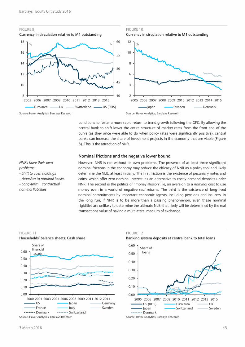
Barclays | Equity Gilt Study 2016
3 March 2016 43
conditions to foster a more rapid return to trend growth following the GFC. By allowing the central bank to shift lower the entire structure of market rates from the front end of the curve (as they once were able to do when policy rates were significantly positive), central banks can increase the share of investment projects in the economy that are viable (Figure 8). This is the attraction of NNR.
Nominal frictions and the negative lower bound However, NNR is not without its own problems. The presence of at least three significant nominal frictions in the economy may reduce the efficacy of NNR as a policy tool and likely determine the NLB, at least initially. The first friction is the existence of pecuniary notes and coins, which offer zero nominal interest, as an alternative to costly demand deposits under NNR. The second is the politics of “money illusion”, ie, an aversion to a nominal cost to use money even in a world of negative real returns. The third is the existence of long-lived nominal commitments by important economic agents, including pensions and insurers. In the long run, if NNR is to be more than a passing phenomenon, even these nominal rigidities are unlikely to determine the ultimate NLB; that likely will be determined by the real transactions value of having a multilateral medium of exchange.
FIGURE 11 Households’ balance sheets: Cash share
FIGURE 12 Banking system deposits at central bank to total loans
Source: Haver Analytics, Barclays Research Source: Haver Analytics, Barclays Research
If equilibrium real rates are negative…
FIGURE 9 Currency in circulation relative to M1 outstanding
FIGURE 10 Currency in circulation relative to M1 outstanding
Source: Haver Analytics, Barclays Research Source: Haver Analytics, Barclays Research
NNRs have their own problems: - Shift to cash holdings - Aversion to nominal losses - Long-term contractual nominal liabilities
0.00
0.10
0.20
0.30
0.40
0.50
0.60
2000 2001 2003 2004 2006 2008 2009 2011 2012 2014
Share of financial assets
US Japan GermanyFrance Italy SwedenDenmark Switzerland
0.00
0.10
0.20
0.30
0.40
0.50
0.60
2005 2006 2007 2008 2010 2011 2012 2013 2015
Share of loans
US (RHS) Euro area UKJapan Switzerland SwedenDenmark
40
45
50
55
60
8
10
12
14
16
18
2005 2006 2007 2008 2010 2011 2012 2013 2015
%%
Euro area UK Switzerland US (RHS)
2
4
6
8
10
12
2005 2006 2007 2008 2009 2010 2012 2013 2014 2015
%
Japan Sweden Denmark

Barclays | Equity Gilt Study 2016
3 March 2016 44
$100 bills as zero-coupon bearer bonds The existence of paper money and coins long has underpinned the belief in a zero lower bound (ZLB) for nominal interest rates. If a central bank – or retail banks – charges interest for holding deposits, people can turn to paper money as an alternative medium of exchange without interest cost. In effect, NNR turns notes and coins into higher-yielding zero-coupon bearer bonds with a maturity of the holder’s choosing. The increasing use of NNR by central banks as a policy tool has demonstrated that there is no ZLB, but the existence of notes and coins is still thought to bound NNR from below at a relatively shallow depth.
The existence of cash as an alternative raises three potential problems for NNR. First, the impact of NNR likely would be muted as economic agents largely or entirely substituted notes and coins for deposits. Second, as depositors shifted to cash, banks may be at risk of deposit flight, which, if widespread, could lead to a collapse of the banking system. Third, even if systemic risks could be contained, the shift away from banks could lead to a breakdown in the payments system.
Empirically, there is little evidence, at least at the moderate level of NNR so far observed, that deposit flight is a significant risk. The currency share of M1 has been falling throughout the G4 and in all NNR economies except Switzerland (Figures 9 and 10). Even in Switzerland, where M1 has fallen since the imposition of NNR (and currency in circulation has risen), there does not appear to be a systemic threat, and one bank has even rolled out NNR on retail transactional deposits without significant loss of deposits.4
Although cash is an alternative to deposits, it is an imperfect substitute and its imperfections likely explain why the ZLB has proven permeable. First, cash has a storage cost, which we have estimated may be as little as 20bp but more realistically may be multiple percentage points (see Three Questions: Quantum Evolution, 27 January 2015). However, although fixed storage in a vault or guarded (and fire-insured) warehouse fulfils two of money’s uses (a unit of account and a store of value) it fails at the third: as a medium of exchange. As transactions are increasingly carried out electronically, not just online but in “bricks-and-mortar” establishments, bank deposits as a medium of exchange are irreplaceable. Hence, although the portion of deposits that represents household savings (see below) may be withdrawn as cash, the portion that is kept for transactional balances likely will remain, even under NNR.
But withdrawing cash as savings to be stored in a vault is not as easy as it sounds, and storage costs likely are only a second- or third-order deterrent; legal restrictions are far more prohibitive. In many developed markets, large cash transactions are illegal, and in all developed countries anti-money laundering laws create serious legal risks – including indefinite asset seizure – for anyone holding or using large sums of cash. 5 Thus, withdrawing cash may not be hard, but using it or returning it to the banking system may be very difficult. For businesses, in particular, this likely means that bank deposits will remain a necessity that will support both the banking and payments systems.
It is tempting to think that storage businesses offering tradable electronic claims would arise as a result, but a business that takes cash deposits in exchange for tradable book entries sounds suspiciously like a bank and likely would run afoul of regulators. Indeed, acquiring enough cash may be difficult: there is not enough to cover M1. Aside from the US – where 50-70% of cash in circulation is abroad6 – in no economy in Figures 9 and 10 does currency comprise more than 16% of M1, and for Japan, Denmark and Sweden it is 5% or less. Under NNR, central banks are unlikely to be incentivized to crank up the actual printing presses to fill
4 “Swiss bank ABS plans negative interest rates for some depositors,” Joshua Franklin, 16 October 2015, Reuters. 5 In the US, authorities have aggressively pursued large cash users with laws that allow seizure of any cash and bank deposits until the accused can prove the legal sources of all funds, a process that can take years. See “Law Lets I.R.S. Seize Accounts on Suspicion, No Crime Required,” Shaila Dewan, The New York Times, 25 October 2014. See also banks’ legal requirements for AML reporting in “Suspicious Activity Reporting – Overview” in Bank Secrecy Act Anti-Money Laundering Examination Manual, Federal Financial Institutions Examination Council. 6 “Crisis and Calm: Demand for U.S. Currency at Home and Abroad from the Fall of the Berlin Wall to 2011,” Ruth Judson, November 2012, International Finance Discussion Papers 1058, Federal Reserve Board of Governors.
Attraction of cash in a NNR world…
… could limit effectiveness of policy and challenges banks as intermediaries
Storage costs for cash could play an important role

Barclays | Equity Gilt Study 2016
3 March 2016 45
large orders for notes (as opposed to the figurative printing press for reserves). The SNB reportedly has encouraged Swiss banks not to accommodate cash withdrawals.7
This last point hits upon a broader reason why the existence of notes and coins is unlikely to be the limiter of NNR, if the sovereign backs its use by central banks. Ultimately, the sovereign makes the rules. A determined sovereign can use myriad methods to undermine cash as an alternative, including – in the era of e-commerce – removing notes and coins from circulation altogether. While there is bound to be popular resistance to government efforts to remove cash from circulation, governments have a strong fiscal (and criminal-justice) incentive to do so as it forces the black-market economy into the light where it cannot evade taxes.
The politics of “money illusion”: charging for money Beyond whether or not sovereign peoples will support their respective central banks in restricting cash usage, a more important question determining both the future of NNR and the NLB is if they will support NNR on retail deposits, a necessary step for NNR to be effective policy at more deeply negative levels.
There are three key hurdles to retail NNR. First, and most important, “money illusion” – people’s greater aversion to nominal losses than real losses – creates a political barrier for banks to institute NNR on retail deposits. Second, there is a “first mover” disadvantage for banks: the first bank to impose retail NNR is at risk of deposit flight (to other banks, not cash), making it difficult to initiate retail NNR in an economy. Third, and of great recent concern to markets, without retail pass-through, deeper NNR either puts banks’ profitability at risk or requires them to raise lending rates – constricting lending – to offset the higher-than-market funding cost of deposits and negative rates incurred on liquid assets required by regulation (see Implications section for a more detailed review of the effects of NNR on banks).
Although retail depositors in most countries have in recent years faced persistent negative real rates of returns on their deposits, due to the “money illusion” people have a strong aversion to accepting nominal losses. Even low nominal interest rates – rather than negative real returns – have drawn protests against QE, particularly in high-savings countries and political constituencies. For this reason, most banks in NNR economies have resisted passing NNR on to depositors other than for institutional deposits and very large retail deposits. In several European countries, NNR is illegal on retail deposits, and some in the US Congress have questioned even the Fed’s legal ability to institute negative rates on reserves of banks.8
Political constraints accentuate the “first mover” problem. Without the political problems created by money illusion, central banks as regulators could push banks to move in unison toward retail NNR. But a central bank that encourages retail banks to charge retail depositors NNR raises its political exposure and threatens its independence. Yet, events may force action. As noted above, in Switzerland the SNB has discouraged banks from providing cash to large, institutional depositors (who are exposed to NNR on deposits and market instruments). Eventually, such policies are likely to create a political debate that either will result in political legitimacy for retail NNR or lead to curtailment of the SNB’s policy of NNR. Similarly, we have argued that a surge in the exchange value of the CHF may push the SNB to force banks toward retail NNR (on a largely foreign deposit base) by removing the exemptions it currently allows domestic banks from NNR on their sight deposits (reserves at the SNB).
One metric of the likely political risk from NNR is the share of household financial assets that are kept in some form of deposit. Switzerland is in the middle of the pack, with about 30% of household financial assets held as bank deposits or currency, a level roughly on par with France and Italy, but significantly below the almost 40% held by German residents. However, the most politically exposed to retail NNR would appear to be the BoJ as Japanese households keep more than 50% of financial assets as currency and deposits. However, the
7 “Negativzins: Bank verweigert Pensionskasse Bargeld-Auszahlung,” Rahel Sahli, 12 March 2015, Schweizer Radio und Fernsehen. 8 “Yellen Re-Examining Negative Rates; Top Lawmaker Doubts Legality,” Matthew Boesler and Jana Randow, 11 February, 2016, BloombergBusiness.
Sovereign can ultimately limit avoidance-schemes (ie, flight to cash)
NNRs have not been passed on to retail depositors… …and ‘first mover ‘ bank could risk deposit flight Could NNRs losses force banks to increase lending rates?
Switzerland could eventually remove exemptions on retail deposits
Japanese households have very large deposit holdings
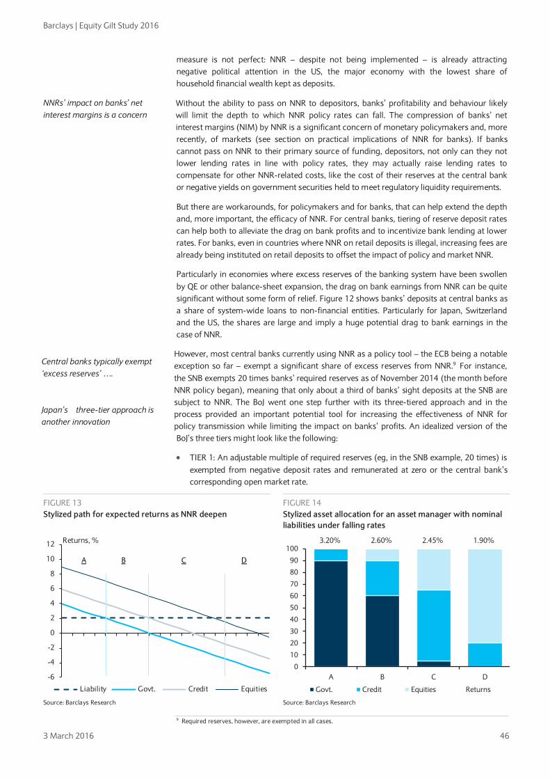
Barclays | Equity Gilt Study 2016
3 March 2016 46
measure is not perfect: NNR – despite not being implemented – is already attracting negative political attention in the US, the major economy with the lowest share of household financial wealth kept as deposits.
Without the ability to pass on NNR to depositors, banks’ profitability and behaviour likely will limit the depth to which NNR policy rates can fall. The compression of banks’ net interest margins (NIM) by NNR is a significant concern of monetary policymakers and, more recently, of markets (see section on practical implications of NNR for banks). If banks cannot pass on NNR to their primary source of funding, depositors, not only can they not lower lending rates in line with policy rates, they may actually raise lending rates to compensate for other NNR-related costs, like the cost of their reserves at the central bank or negative yields on government securities held to meet regulatory liquidity requirements.
But there are workarounds, for policymakers and for banks, that can help extend the depth and, more important, the efficacy of NNR. For central banks, tiering of reserve deposit rates can help both to alleviate the drag on bank profits and to incentivize bank lending at lower rates. For banks, even in countries where NNR on retail deposits is illegal, increasing fees are already being instituted on retail deposits to offset the impact of policy and market NNR.
Particularly in economies where excess reserves of the banking system have been swollen by QE or other balance-sheet expansion, the drag on bank earnings from NNR can be quite significant without some form of relief. Figure 12 shows banks’ deposits at central banks as a share of system-wide loans to non-financial entities. Particularly for Japan, Switzerland and the US, the shares are large and imply a huge potential drag to bank earnings in the case of NNR.
However, most central banks currently using NNR as a policy tool – the ECB being a notable exception so far – exempt a significant share of excess reserves from NNR.9 For instance, the SNB exempts 20 times banks’ required reserves as of November 2014 (the month before NNR policy began), meaning that only about a third of banks’ sight deposits at the SNB are subject to NNR. The BoJ went one step further with its three-tiered approach and in the process provided an important potential tool for increasing the effectiveness of NNR for policy transmission while limiting the impact on banks’ profits. An idealized version of the BoJ’s three tiers might look like the following:
• TIER 1: An adjustable multiple of required reserves (eg, in the SNB example, 20 times) is exempted from negative deposit rates and remunerated at zero or the central bank’s corresponding open market rate.
9 Required reserves, however, are exempted in all cases.
NNRs’ impact on banks’ net interest margins is a concern
Central banks typically exempt ‘excess reserves’ …. Japan’s three-tier approach is another innovation
FIGURE 13 Stylized path for expected returns as NNR deepen
FIGURE 14 Stylized asset allocation for an asset manager with nominal liabilities under falling rates
Source: Barclays Research
Source: Barclays Research
-6
-4
-2
0
2
4
6
8
10
12 Returns, %
Liability Govt. Credit Equities
A B C D
3.20% 2.60% 2.45% 1.90%
0
10
20
30
40
50
60
70
80
90
100
A B C D
Govt. Credit Equities Returns

Barclays | Equity Gilt Study 2016
3 March 2016 47
• TIER 2: An additional “macro add-on” balance tied to banks’ lending activity that, like Tier 1, would be remunerated at zero or the central bank’s open market policy rate.
• TIER 3: Remaining excess liquidity would be fully subject to the negative deposit rate.
So long as Tiers 1 and 2 are less than the total reserves of the system, excess liquidity will pressure marginal funding costs of both the banking system and financial system toward the central bank’s negative deposit rate due to Tier 3 reserve treatment. But the adjustable proportion of required reserves in Tier 1 allows the central bank to exempt the majority of system reserves – even when excess reserves are large – reducing banks’ average cost of NNR and thus reducing the overall impact on banking system profitability.
More important, the innovation of Tier 2 gives central banks an effective tool to encourage banks to lend more and to pass lower interest costs on to non-financial borrowers. An example helps to illustrate the power of such a system: under zero nominal rates and QE, banks’ only incentive to lend more is the opportunity cost of returns on loans relative to government securities. But with the three-tiered system above and NNR, banks would have an additional incentive: they could reduce, dollar-for-dollar, their associated NNR costs on reserves by lending to the non-financial economy. For instance, for a central bank deposit rate of -1%, a bank could reduce NNR costs by 100pb per dollar of excess reserves for every dollar lent as this would shift Tier 3 reserves to Tier 2 reserves, an effective 100bp subsidization of lending rates.
This tiered mechanism gives the bank several levers to operate both on the economy and on bank profits. By adjusting the proportion of reserves included in Tier 1 and the rate of remuneration on Tier 1 reserves, the central bank can increase or decrease the relief banks receive from NNR on average on a system-wide basis. By adjusting the multiple of new lending for which banks can transform Tier 3 reserves into Tier 2 reserves, and by adjusting the rates of interest between those two tiers, the central bank can increase or decrease the incentive for banks to expand lending activity. This may be particularly useful for central banks that have coincident macro-prudential or financial stability mandates. Finally, by adjusting the NNR deposit rate on Tier 3 reserves and the total quantity of reserves of the system, the central bank can adjust the marginal cost of finance for the financial system as a whole, its traditional tool of monetary policy.
The increased ability to spur banks to lend and the reduction in effective NNR burden from reserves would give central banks extra leeway to reduce policy rates more deeply into NNR even without pass-through to retail depositors. However, there is a limit: as long as bank deposits yield zero, the further market rates descend with the Tier 3 deposit rate, the more banks will face increasing deposit inflows. To some extent, those can be deterred by increasing account fees, but it is a lagging, inefficient mechanism that likely has its own limits in a society that does not accept retail NNR.
It is worth mentioning that concerns about the viability of money market funds or oft-cited institutional constraints around those are unlikely to constrain NNR, even with retail deposits still yielding zero. Regulations that prohibit money market funds from “breaking the buck”, ie, returning less than invested, as is the case in the US, can be changed if needed (not that we expect the US to move to negative rates; see Coping with negativity, 8 November 2012, for a fuller discussion of US institutional barriers to negative rates). Although retail deposits may leave money market funds for zero-yielding bank deposits, as has already occurred in existing NNR countries, large and institutional deposits will be forced by the bank fees or NNR pass-through to go elsewhere, and, when liquidity is important, likely to money market funds.
Long-term nominal liabilities under negative nominal rates A firmer foundation for the NLB may be more associated with the nominal liabilities of insurers and pensions. Furthermore, the boundary created by long-term nominal commitments has important implications for risk premia, including credit spreads and the equity risk premium (ERP).
Pressuring marginal but reducing average costs
Incentivize banks to lend more
Adjusting ‘tiers’ becomes part of monetary policy

Barclays | Equity Gilt Study 2016
3 March 2016 48
FIGURE 15 Stylized path of risk premia as nominal-liability constrained asset managers “chase yield”
Source: Barclays Research
To understand this constraint and its asset price implications, think about entities with long-lived nominal liabilities and low risk tolerance, eg, pensions and insurers. Figures 13, 14 and 15 illustrate the impact of increasingly negative rates on, respectively, their return opportunities, their portfolio choices, and market risk spreads, segmented into four phases. In a “normal” world with historically observed nominal government bond yields (phase A), they invested mostly in government bonds, with some investment grade credit to meet their nominal commitments, or in the case of non-mutualised insurers to earn a small return over nominal commitments.
But as yields fall below their required rate of nominal return (phase B), they increase their risk by shifting their allocation toward credit as a yield investment to match their liabilities rather than as a spread product. This exerts downward pressure on credit spreads. Phase B is effectively what has occurred at pensions and insurers already under QE. As NNRs are introduced and go progressively deeper (phase C) the process continues until yields on investment grade credit also fall below required rates of return. At that point, any further declines in rates would require an increase in spread to meet insurers’ and pensions’ minimum yield, meaning that investment grade spreads bottom out and begin to rise as rates go even more negative. Meanwhile, insurers and pensions – subject to regulatory allowances – push even further out the risk curve to meet their nominal obligations, repeating the same process for high yield spreads, and eventually the equity risk premium.
But at some point (phase D), further declines in rates – and risk spreads – imply that returns, even on risky portfolios, are insufficient to meet their long-term nominal commitments, which simultaneously are rising in net present value as interest rates fall. This process is accelerated by the existence of regulatory barriers to further risk-taking. At that point, pensions and insurers are insolvent and need to turn to their regulator or the state either for capital injections or for contractual relief from their nominal liabilities (both of which have fiscal implications, as discussed below). Pensions and insurers entering regulatory protection or receivership are unlikely to be allowed to take on further risk, and likely will be forced to actively de-risk, sending credit spreads and the ERP sharply higher as the financial system’s marginal buyers turn to sellers.
The ultimate NLB: the transactions value of money But, as we noted in Three Questions: Quantum Evolution, 27 January 2015, it is the utility of transactions demand that likely dictates the ultimate NLB. Even once political obstacles to retail NNR are overcome and long-term nominal constraints have been dealt with, the transactions value of money is still a barrier. As noted above, although there may exist alternative stores of value and units of account, only legal tender can facilitate multilateral transactions (rather than barter) in a sovereign society that accepts NNR.
0
1
2
3
4
5
6
7
8
9
+ 0 -Credit risk premium Equity risk premium Hurdle Rate
Issuers default Investors default
A B C D
Real interest rates
Those with long-term nominal contractual commitment under increased pressure…
… as their need for yield pushes them into riskier instruments, which in turn further compresses spreads…
…and at some point will no longer suffice to meet nominal obligations

Barclays | Equity Gilt Study 2016
3 March 2016 49
The convenience value of multilateral exchange likely forms the NLB. A measure of how much that transaction utility is worth to consumers and to businesses may be given by credit and debit card interchange fees, the fee that card companies charge merchants for transactions. Until recent moves to regulate interchange fees, such fees on debit cards were around 1-3 percent of transaction value, depending on the card and the merchant. Credit cards, which remain unregulated, still command fees in that range, with some reaching as high as 6%. Coincidentally, the ECB has calculated that the social welfare value of such transactions is 2.3%.10 If these rates represent an accurate measure of transaction utility, they suggest that the ultimate NLB for interest rates likely is considerably lower than the -125bp charged on reserves deposited at the Swedish Riksbank (currently the lowest policy rate).
Given the current constraints, how low can NNR reasonably go? Until retail NNR becomes politically feasible and governments establish credible plans to deal with the adverse impact on pensions and insurers, it seems unlikely that NNR would be able to fall much below the Riksbank’s -125bp deposit rate in most economies, and perhaps not even that low in countries with high levels of retail bank deposits (eg, Japan) or large, contingent long-term commitments (eg, Germany). Even with tiered reserve charges, in the absence of retail NNR, the pressure on bank deposit inflows may require unrealistic (or politically infeasible) fees on deposits, and insurers and pensions are already creaking under the strain of their nominal commitments amid historically low fixed income yields.
Economic policy below the zero
Monetary policy with negative nominal rates Monetary policy under NNR, at least in theory, should be more familiar and have more direct transmission than other unconventional policies as it returns central banks to their pre-crisis (positive interest rate) world of adjusting the marginal cost of short-term funding in the economy. Relative to changing interest rates above the ZLB, however, there likely are some differences in effect and nagging unknowns regarding NNR as a policy tool. Among these are: 1) if retail NNR is not politically feasible, the ZLB on retail deposits likely induces some frictions that could slow or impair the transmission of monetary policy; 2) the existence of long-term nominal commitments, as discussed above, may raise rather than lower risk spreads beyond some threshold for NNR policy rates; 3) uncertainty about the existence and depth of the NLB may reduce policy effectiveness by raising risk premia and impairing market expectations for the forward path of monetary policy; 4) conversely, if uncertainty increases FX risk premia, a move to NNR may yield a larger-than-usual depreciation of the exchange rate, improving the FX channel of transmission; 5) money illusion may reduce wealth effects usually associated with monetary policy when interest “income” becomes a payment or is amortized as a reduction in principal. Furthermore, as with any untried policy, there may well be unanticipated effects.
Figure 16 presents a stylized view of monetary policy as it descends below the ZLB. Above zero, the central bank adjusts the reserves of the banking system (𝑅0 ) along the money/loan demand curve of the economy (𝑀𝐷/𝐿𝐷)11 to achieve the desired level of lending and economic activity at target policy rate 𝑖+. But at the ZLB, adding more reserves to the banking system (𝑅1) only increases excess reserves (𝑋𝑆1) because money/loan demand will not expand beyond point A without a further decline in interest rates. At this point, if the central bank introduces a cost to holding excess reserves – a negative deposit rate, 𝑖− –
10 See “Life below zero: Learning about negative interest rates,” speech by Benoit Cœuré, ECB Executive Board Member, 9 September 2014, Frankfurt am Main, Germany; and “The social and private costs of retail payment instruments. A European perspective,” H. Schmiedel, G. Kostova, and W. Ruttenberg, 2012, ECB Occasional Papers Series , No. 137. 11 We describe this as a money/loan demand curve because the effect on measured monetary aggregates is ambiguous. Particularly in the case where retail NNRs are allowed, measures of money like M1 may contract as households reduce their savings portfolio allocation to money, reducing money balances, but begin to use remaining transactional money balances more efficiently, ie, the velocity of money increases. Thus, measured money balances may contract, but loans outstanding and economic activity increase. For economic activity and inflation, it is the product of money and velocity that matters, not the quantity of money.
Credit card charges as lower bound for NNRs?
Swedens’ -125bp deposit rate may be close to what is feasible in practice
Theoretical elegance of NNRs are challenged by many real-life challenges
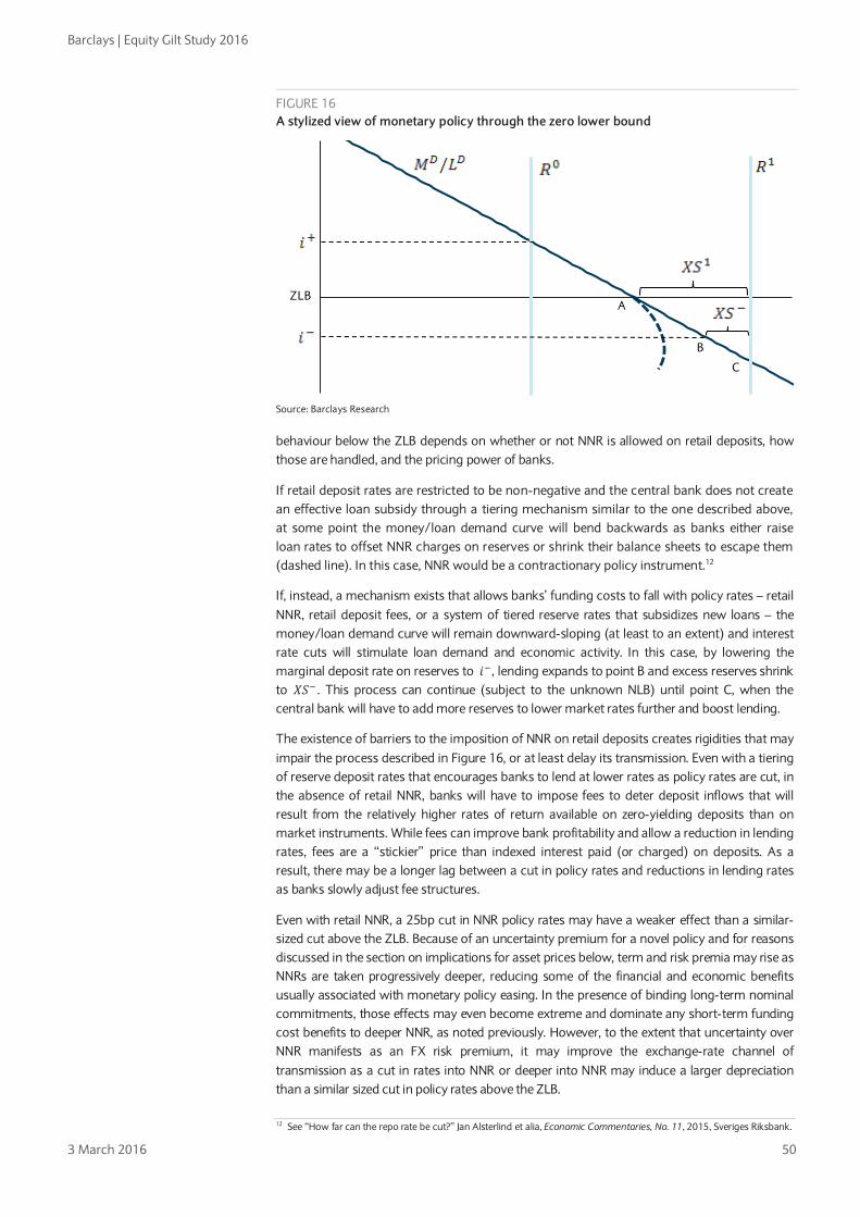
Barclays | Equity Gilt Study 2016
3 March 2016 50
behaviour below the ZLB depends on whether or not NNR is allowed on retail deposits, how those are handled, and the pricing power of banks.
If retail deposit rates are restricted to be non-negative and the central bank does not create an effective loan subsidy through a tiering mechanism similar to the one described above, at some point the money/loan demand curve will bend backwards as banks either raise loan rates to offset NNR charges on reserves or shrink their balance sheets to escape them (dashed line). In this case, NNR would be a contractionary policy instrument.12
If, instead, a mechanism exists that allows banks’ funding costs to fall with policy rates – retail NNR, retail deposit fees, or a system of tiered reserve rates that subsidizes new loans – the money/loan demand curve will remain downward-sloping (at least to an extent) and interest rate cuts will stimulate loan demand and economic activity. In this case, by lowering the marginal deposit rate on reserves to 𝑖−, lending expands to point B and excess reserves shrink to 𝑋𝑆− . This process can continue (subject to the unknown NLB) until point C, when the central bank will have to add more reserves to lower market rates further and boost lending.
The existence of barriers to the imposition of NNR on retail deposits creates rigidities that may impair the process described in Figure 16, or at least delay its transmission. Even with a tiering of reserve deposit rates that encourages banks to lend at lower rates as policy rates are cut, in the absence of retail NNR, banks will have to impose fees to deter deposit inflows that will result from the relatively higher rates of return available on zero-yielding deposits than on market instruments. While fees can improve bank profitability and allow a reduction in lending rates, fees are a “stickier” price than indexed interest paid (or charged) on deposits. As a result, there may be a longer lag between a cut in policy rates and reductions in lending rates as banks slowly adjust fee structures.
Even with retail NNR, a 25bp cut in NNR policy rates may have a weaker effect than a similar-sized cut above the ZLB. Because of an uncertainty premium for a novel policy and for reasons discussed in the section on implications for asset prices below, term and risk premia may rise as NNRs are taken progressively deeper, reducing some of the financial and economic benefits usually associated with monetary policy easing. In the presence of binding long-term nominal commitments, those effects may even become extreme and dominate any short-term funding cost benefits to deeper NNR, as noted previously. However, to the extent that uncertainty over NNR manifests as an FX risk premium, it may improve the exchange-rate channel of transmission as a cut in rates into NNR or deeper into NNR may induce a larger depreciation than a similar sized cut in policy rates above the ZLB. 12 See “How far can the repo rate be cut?” Jan Alsterlind et alia, Economic Commentaries, No. 11, 2015, Sveriges Riksbank.
FIGURE 16 A stylized view of monetary policy through the zero lower bound
Source: Barclays Research
ZLBA
B
C
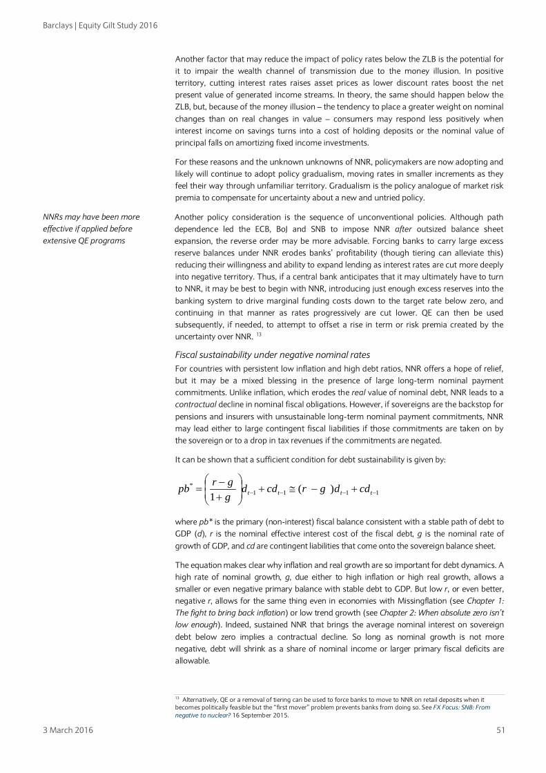
Barclays | Equity Gilt Study 2016
3 March 2016 51
Another factor that may reduce the impact of policy rates below the ZLB is the potential for it to impair the wealth channel of transmission due to the money illusion. In positive territory, cutting interest rates raises asset prices as lower discount rates boost the net present value of generated income streams. In theory, the same should happen below the ZLB, but, because of the money illusion – the tendency to place a greater weight on nominal changes than on real changes in value – consumers may respond less positively when interest income on savings turns into a cost of holding deposits or the nominal value of principal falls on amortizing fixed income investments.
For these reasons and the unknown unknowns of NNR, policymakers are now adopting and likely will continue to adopt policy gradualism, moving rates in smaller increments as they feel their way through unfamiliar territory. Gradualism is the policy analogue of market risk premia to compensate for uncertainty about a new and untried policy.
Another policy consideration is the sequence of unconventional policies. Although path dependence led the ECB, BoJ and SNB to impose NNR after outsized balance sheet expansion, the reverse order may be more advisable. Forcing banks to carry large excess reserve balances under NNR erodes banks’ profitability (though tiering can alleviate this) reducing their willingness and ability to expand lending as interest rates are cut more deeply into negative territory. Thus, if a central bank anticipates that it may ultimately have to turn to NNR, it may be best to begin with NNR, introducing just enough excess reserves into the banking system to drive marginal funding costs down to the target rate below zero, and continuing in that manner as rates progressively are cut lower. QE can then be used subsequently, if needed, to attempt to offset a rise in term or risk premia created by the uncertainty over NNR. 13
Fiscal sustainability under negative nominal rates For countries with persistent low inflation and high debt ratios, NNR offers a hope of relief, but it may be a mixed blessing in the presence of large long-term nominal payment commitments. Unlike inflation, which erodes the real value of nominal debt, NNR leads to a contractual decline in nominal fiscal obligations. However, if sovereigns are the backstop for pensions and insurers with unsustainable long-term nominal payment commitments, NNR may lead either to large contingent fiscal liabilities if those commitments are taken on by the sovereign or to a drop in tax revenues if the commitments are negated.
It can be shown that a sufficient condition for debt sustainability is given by:
1111* )(
1 −−−− +−≅+
+−
= tttt cddgrcddggrpb
where pb* is the primary (non-interest) fiscal balance consistent with a stable path of debt to GDP (d), r is the nominal effective interest cost of the fiscal debt, g is the nominal rate of growth of GDP, and cd are contingent liabilities that come onto the sovereign balance sheet.
The equation makes clear why inflation and real growth are so important for debt dynamics. A high rate of nominal growth, g, due either to high inflation or high real growth, allows a smaller or even negative primary balance with stable debt to GDP. But low r, or even better, negative r, allows for the same thing even in economies with Missingflation (see Chapter 1: The fight to bring back inflation) or low trend growth (see Chapter 2: When absolute zero isn’t low enough). Indeed, sustained NNR that brings the average nominal interest on sovereign debt below zero implies a contractual decline. So long as nominal growth is not more negative, debt will shrink as a share of nominal income or larger primary fiscal deficits are allowable.
13 Alternatively, QE or a removal of tiering can be used to force banks to move to NNR on retail deposits when it becomes politically feasible but the “first mover” problem prevents banks from doing so. See FX Focus: SNB: From negative to nuclear? 16 September 2015.
NNRs may have been more effective if applied before extensive QE programs

Barclays | Equity Gilt Study 2016
3 March 2016 52
However, contingent liabilities may be exacerbated by NNR. Although markets recently have exhibited concerns about the impact of NNR on banks’ sustainability, as noted above, this need not be a problem if retail NNR are feasible or at low levels of NNR, with tiering of central bank charges on reserves. But long-term nominal commitments of pensions and insurers likely are more difficult to deal with under NNR. With sustained NNR, many pensions and insurers likely are not viable and either will need a fiscal backstop or contractual relief from their nominal commitments. In the former case, cd may boost the fiscal debt by more than a decline in r improves long-run debt dynamics. In the latter case, the breaking of pensions’ and insurers’ nominal commitments implies lower future government tax revenues and perhaps increased social welfare payments, permanently raising primary fiscal deficits.
Financial stability concerns An oft cited concern with respect to NNR and other unconventional monetary policies is their impact on financial stability and their potential to create asset bubbles. However, these concerns are not unique to unconventional policies or NNR. Rather, they are a general critique of the risks of pursuing excessively easy monetary policy, whether above the ZLB or below.
Key economic policymakers have expressed concerns that NNR and other unconventional monetary policies have depressed real interest rates below the “Wicksellian natural rate” that equates savings with investment.14 However, such assessments do not accord well with the data. In most developed economies, saving rates are rising and investment growth has remained stubbornly below expected rates despite historically low rates of interest. An unusually large cohort of high-earning middle-aged workers nearing retirement appears to be more the problem as their savings are increasing faster than their demand for goods and services (see Chapter 4: Population dynamics and global imbalances).
High asset prices are a consequence of low real interest rates, not monetary policy “leaking” into asset price rather than consumer price inflation. If central banks had successfully reduced real interest rates below their Wicksellian natural level, investment activity would be much stronger, generating production bottlenecks and goods and services inflation. Widespread resource slack and lack of inflation suggest this is not a common problem.
Concluding thoughts Negative nominal rates have the potential to be a powerful new tool in central banks’ arsenal in a world where real risk-free interest rates appear to have slipped below zero and Missingflation plagues a wide spectrum of economies. There still are significant hurdles to NNRs realizing their full potential. Most important, central banks will need to confront the politics of money illusion and of passing NNR on to retail depositors if it is to be as effective a tool in practice as it promises in theory. Tiering of reserve balances provides a powerful workaround to resistance to retail NNR, but can only allow rates to descend so far. A greater problem, particularly in economies with large legacy long-term nominal commitments at pension funds and insurers, may be the social and fiscal costs of those institutions’ insolvency. However, with no end to negative real rates or Missingflation in sight, negative nominal rates have – excuse the pun – a very positive future, in our assessment.
14 See “World faces wave of epic debt defaults, fears central bank veteran,” Ambrose Evans-Pritchard, The Telegraph, 19 January 2016; or “Ultra-low or negative interest rates: what they mean for financial stability and growth” Hervé Hannoun, Deputy General Manager, Bank for International Settlements, remarks at Eurofi High-Level Seminar, Riga, 22 April 2015.

Barclays | Equity Gilt Study 2016
3 March 2016 53
CHAPTER 4
Population dynamics and global imbalances • Concerns about large and persistent current account imbalances (and the net capital
flows underlying them) have been displaced by more pressing issues associated with the global financial crisis. But the imbalances have persisted and have recently begun to expand again. We think these longstanding imbalances are associated with structural (as opposed to cyclical) influences on national propensities to save, and that demographic developments are a key driver of these propensities. We find a strong positive correlation between average external imbalances over the past 20 years and a measure of demographic support for saving.
• Last year, we presented evidence that the three-decade slide in the world real interest rate was largely attributable to population dynamics in those economies comprising the bulk of global economic activity, savings, and investment, and that the extended period of support for asset prices was on the cusp of a slow but sizeable reversal. Building on that research, we now extend our framework to explore linkages between prospective population dynamics and external imbalances, focusing on how demographic developments are likely to affect imbalances.
• For the world’s largest economies, we find that prospective demographic developments do not suggest a large change in the pattern of net capital flows and current account imbalances because the shifts in national demographic trends are reasonably well synchronized. In particular, population dynamics suggest that China and the European Union will likely remain capital exporters in the coming 10-15 years, while the US and UK are likely to remain net capital importers. In some smaller countries, including Korea, Russia, and Latin America, we project more substantial effects on net capital flows and current account imbalances.
In last year’s Study, we suggested that global population dynamics provide a coherent explanation for the ‘global savings glut’ that, in our view, lies behind the 30-year decline in the ‘natural’ rate of interest and, more generally, the secular updraft in asset values over the same period. In a follow-up note, we quantified the impact of demographic pressure for saving on the ‘natural’ rate of interest, and suggested that demographic trends could explain most of the secular decline in the real interest rate since the mid-1980s. We also argued that the ongoing global demographic transition is likely to be accompanied by a secular rise in interest rates and downward pressure on asset prices in the decades ahead.
Michael Gavin +1 212 412 5915 [email protected] BCI, US
FIGURE 1 The US and China are, quantitatively, the most important drivers of ‘global imbalances’…
FIGURE 2 … but in 1995-2014, current accounts have been large where demographic support for saving has been strong
Source: Haver Analytics, Barclays Research Source: Haver Analytics, Barclays Research
We find a strong positive correlation between average external imbalances over the past 20 years and a measure of demographic support for saving
-2.0%
-1.5%
-1.0%
-0.5%
0.0%
0.5%
1.0%
1.5%
1995
1997
1999
2001
2003
2005
2007
2009
2011
2013
2015
CAS/World GDP
China US CHN + KOR, BRA, RUS
US
China
Euro area
Japan
UKIndia
Korea
Brazil
Mexico
Russia
-4.0%
-2.0%
0.0%
2.0%
4.0%
6.0%
8.0%
0.14 0.16 0.18 0.20 0.22
CAS/GDP
Demographic pressure (middle-old)

Barclays | Equity Gilt Study 2016
3 March 2016 54
If these population dynamics were evolving uniformly around the world, we would not have much more to say. However, a key aspect of the demographic transition is that it is not proceeding at the same pace across regions, thereby placing disparate pressures on saving and investment in different parts of the world. This suggests that population dynamics are a plausible driver of the current account imbalances that have puzzled analysts and vexed policymakers in recent decades. In this section, we extend our framework to explore linkages between demographics and external imbalances, with a specific focus on how demographic developments are likely to affect these relationships.
Global imbalances – Trend and cycle In the run-up to the global financial crisis and subsequent recession, a key preoccupation of policymakers and source of uncertainty for investors was the growth of ‘global imbalances’. Quantitatively, the most important of these were the US current account deficit, which expanded to a peak of roughly 6% of GDP (1.5% of world GDP) in 2006, and the Chinese current account surplus, which peaked at c.10% of GDP (nearly 1% of world GDP) in 2007.
Although other, mainly smaller, economies have, individually, been less significant drivers of global current account flows, they have collectively played a significant role. For example, between 1996-97 (before the Asian financial crisis) and 2005-06, the combined current account balances of Korea, Russia, and Brazil rose by nearly 0.5% of world GDP, mainly because of the capital outflows that followed that crisis. These outflows were particularly large and persistent in Russia, where a subsequent strong recovery in energy prices also bolstered exports and the current account.
As this very brief account of the historical backdrop shows, global current account imbalances have been strongly affected by short-term, broadly defined ‘cyclical’ influences, particularly the impact on desired international capital flows of economic and financial crises, major fluctuations in energy and other commodity prices, and the turbo-charged financial environment that led up to the 2007 global financial crisis. We do not focus on these here, largely because they are hard to forecast, even if they are fully understood.
However, persistent ‘structural’ influences are also clearly at work. On the one hand, apart from a two-quarter blip in the early 1990s, the US has not run a quarterly current account surplus since the early 1980s. Of smaller systemic significance, Brazil, India, Mexico and the UK have also tended persistently to run current account deficits. On the other hand, since its emergence as a systemically important economy, China has consistently generated current account surpluses, and, although the unusually high surpluses of the mid-2000s have given way to more normal levels, the Chinese surplus remains at a significant 0.5% of world GDP. In the past several years, Germany and Korea have also emerged as chronic surplus economies, for reasons that are difficult to explain as transitory ‘cyclical’ factors, while Japan’s tendency to generate moderate current account surpluses has vanished in the past half-decade.
One potential driver of these persistent, apparently ‘structural,’ current account imbalances is saving, particularly demographic influences on the propensity to save. It is natural to consider saving as a determinant of the current account balance because the current account is, as a matter of national income accounting, equal to the difference between domestic saving and investment. Thus, a fundamental driver that raises domestic saving will generate a current account surplus, unless it also spurs correspondingly higher investment.
In last year’s Study, we presented evidence (consistent with previous studies of national saving) that demographic structure is an important driver of national saving. Specifically, national saving tends to be higher in countries whose population has a large share of mature, typically high-saving workers (measured in our analysis as the share of the population between the ages of 40 and 64), and it tends to be lower in economies with a high share of elderly people (measured as the share of the population aged 65 and older).
Global current account imbalances have been strongly affected by short-term ‘cyclical’ influences…
…but persistent ‘structural’ influences are also clearly at work

Barclays | Equity Gilt Study 2016
3 March 2016 55
As a summary measure of demographic pressure on saving, we use the difference between the population shares of high-saving mature workers and of the elderly.1
Figure 2 provides some evidence that demographic structure has in fact been correlated with longer-run current account developments. The vertical axis plots the average current account balance, measured as a share of GDP, in 1995-2014; the horizontal axis plots the measure of demographic pressure on saving described above.
There is a strong positive correlation between demographic fundamentals and current accounts. Of course, this measure of demographic pressure does not provide a complete explanation of cross-country current account dynamics. The biggest outlier is Russia, where the extraordinarily large capital outflows that followed the 1998 economic crisis skew the average higher, for reasons that are not captured by an analysis that focuses on demographic or other fundamentals.
A framework We use a simple Fisherian model of the natural rate of interest, with two financially integrated economies, to illustrate some of the points we have explored (Figure 3). In each economy investment demand is a decreasing function of the real interest rate. The investment demand schedule for the home country is drawn in the right section as I(r), and the rest of the world’s investment demand is drawn in the left panel as I*(r), with an increase in ROW investment represented by a move to the left, away from the origin of the axes.
FIGURE 3 An increase in domestic saving, with international spillovers
Source: Barclays Research
Similarly, the supplies of domestic and foreign savings are drawn as the upward-sloping curves S(r) and S*(r), respectively. The equilibrium rate of interest is determined by the condition that world saving equals world investment, or, equivalently, that the home country’s current account surplus equals the rest of the world’s deficit.
In Figure 3, we have drawn a hypothetical equilibrium where the current account is equal to zero in both countries. We then consider some shift in fundamentals that increases the home country’s propensity to save. As a result of this shift, the world interest rate falls, and world investment therefore rises. Domestic saving rises and the current account moves into surplus, but foreign saving falls, with the resulting ROW current account deficit (CA*) matching the surplus in the home country (CA).
1 In our more formal statistical work, we estimated the separate effects of the two demographic variables on saving. On the basis of our finding that one variable has approximately the same effect as the other, but with the opposite sign, we feel comfortable using the difference between the variables as a summary measure, as in Figure 2.
There is a strong positive correlation between demographic fundamentals and current accounts, though this does not completely explain cross-country current account dynamics

Barclays | Equity Gilt Study 2016
3 March 2016 56
Simplistic though the framework may be, it highlights that a relationship between one country’s demographic fundamentals and its current account, as in Figure 3, is not a simple, fixed relationship because the current account (and therefore domestic saving and investment) is also determined by demographic fundamentals in the rest of the world. To calibrate the potential impact of demographic drivers on external imbalances requires that we account for these international spillovers. This is particularly germane in the present context, in which demographic support for saving is set to fade in most of the world in the decades to come. As it does so, every economy’s current account cannot deteriorate simultaneously.
Looking ahead It is not difficult to quantify a multi-national application of this two-country theoretical framework and, given projections of populations’ age structures, to estimate the impact of demographic developments on equilibrium current account imbalances in the years ahead. As noted, current account imbalances are determined by many factors besides the demographic developments we focus on here. The projections we make should be viewed as estimated effects of prospective demographic changes on ‘structural’ current accounts, not precise forecasts of future imbalances, which will be affected by factors beyond the ones we quantify here.
Our approach is as follows:
• We begin with the assumption that 2015 current account imbalances were more or less consistent with demographic and other structural drivers. This assumption is not particularly important, so long as it is understood that differences between the projected current account balances and the 2015 level represent an estimate of future changes attributable to changes in the age composition of populations in the 10 economic regions included in our analysis.
• We make assumptions about the slope of the saving and investment schedules in Figure 3 and the magnitude of the shift in the schedules that may be attributed to changes in demographic pressure on saving as we have quantified it.2
• For each country, in each year of the projection period, we compute the gap between saving and investment that would result for some arbitrary world interest rate, given the projected demographic structure of each country in that year.
• We then adjust the world interest rate as required to set the aggregate current account to zero.3
The results of this exercise are summarized in Figure 4. For the world’s largest economies, the impact of demography on projected imbalances is modest in the decade ahead, and only slightly larger in the subsequent decade. This reflects the fact that all of these large economies are facing a gradual decline in demographic support for saving, as we have noted in past publications. This means that the most marked effect of the coming demographic transition is likely to be on world interest rates and asset prices, with smaller consequences for global imbalances.
The effect of demographic change is small, but not negligible. For example, our projections suggest that the US and the UK will likely remain capital-importing economies for the foreseeable future and, indeed, that prospective demographic forces will likely intensify this
2 In particular, we assume that a 1pp increase in the real interest rate would increase net saving (the difference between desired supply of saving and the demand for domestic investment) by 0.5% of GDP. This is roughly in line with the assumption made in our previous discussions of this issue. For our current purposes, it is not very important, because it affects only the magnitude of the increase in the interest rate that is required to match world saving and investment; that was our focus in the previous notes, but not this one. We also assume that a 1pp increase in our measure of demographic pressure on saving would boost net saving by 0.5% of GDP, at any constant rate of interest. 3 More precisely, recognizing that the 10 economies that we analyze here do not comprise the entire world, we maintain the aggregated current account balance at its 2015 level, which was roughly 0.4% of world GDP.
The effect of demographic change is small but not negligible
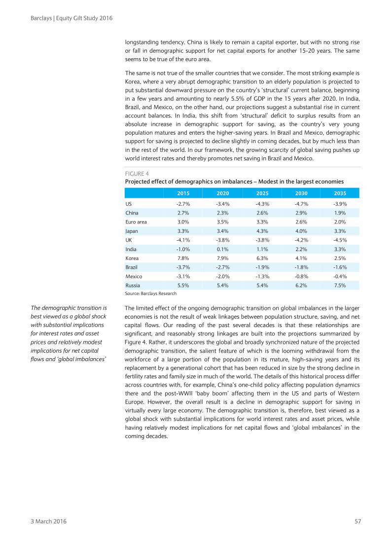
Barclays | Equity Gilt Study 2016
3 March 2016 57
longstanding tendency. China is likely to remain a capital exporter, but with no strong rise or fall in demographic support for net capital exports for another 15-20 years. The same seems to be true of the euro area.
The same is not true of the smaller countries that we consider. The most striking example is Korea, where a very abrupt demographic transition to an elderly population is projected to put substantial downward pressure on the country’s ‘structural’ current balance, beginning in a few years and amounting to nearly 5.5% of GDP in the 15 years after 2020. In India, Brazil, and Mexico, on the other hand, our projections suggest a substantial rise in current account balances. In India, this shift from ‘structural’ deficit to surplus results from an absolute increase in demographic support for saving, as the country’s very young population matures and enters the higher-saving years. In Brazil and Mexico, demographic support for saving is projected to decline slightly in coming decades, but by much less than in the rest of the world. In our framework, the growing scarcity of global saving pushes up world interest rates and thereby promotes net saving in Brazil and Mexico.
FIGURE 4 Projected effect of demographics on imbalances – Modest in the largest economies
2015 2020 2025 2030 2035
US -2.7% -3.4% -4.3% -4.7% -3.9%
China 2.7% 2.3% 2.6% 2.9% 1.9%
Euro area 3.0% 3.5% 3.3% 2.6% 2.0%
Japan 3.3% 3.4% 4.3% 4.0% 3.3%
UK -4.1% -3.8% -3.8% -4.2% -4.5%
India -1.0% 0.1% 1.1% 2.2% 3.3%
Korea 7.8% 7.9% 6.3% 4.1% 2.5%
Brazil -3.7% -2.7% -1.9% -1.8% -1.6%
Mexico -3.1% -2.0% -1.3% -0.8% -0.4%
Russia 5.5% 5.4% 5.4% 6.2% 7.5% Source: Barclays Research
The limited effect of the ongoing demographic transition on global imbalances in the larger economies is not the result of weak linkages between population structure, saving, and net capital flows. Our reading of the past several decades is that these relationships are significant, and reasonably strong linkages are built into the projections summarized by Figure 4. Rather, it underscores the global and broadly synchronized nature of the projected demographic transition, the salient feature of which is the looming withdrawal from the workforce of a large portion of the population in its mature, high-saving years and its replacement by a generational cohort that has been reduced in size by the strong decline in fertility rates and family size in much of the world. The details of this historical process differ across countries with, for example, China’s one-child policy affecting population dynamics there and the post-WWII ‘baby boom’ affecting them in the US and parts of Western Europe. However, the overall result is a decline in demographic support for saving in virtually every large economy. The demographic transition is, therefore, best viewed as a global shock with substantial implications for world interest rates and asset prices, while having relatively modest implications for net capital flows and ‘global imbalances’ in the coming decades.
The demographic transition is best viewed as a global shock with substantial implications for interest rates and asset prices and relatively modest implications for net capital flows and ‘global imbalances’
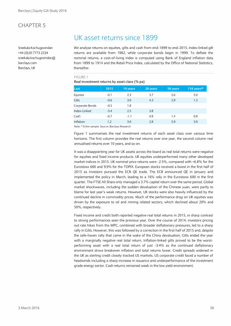
Barclays | Equity Gilt Study 2016
3 March 2016 58
CHAPTER 5
UK asset returns since 1899 We analyse returns on equities, gilts and cash from end-1899 to end-2015. Index-linked gilt returns are available from 1982, while corporate bonds begin in 1999. To deflate the nominal returns, a cost-of-living index is computed using Bank of England inflation data from 1899 to 1914 and the Retail Price Index, calculated by the Office of National Statistics, thereafter.
FIGURE 1 Real investment returns by asset class (% pa)
Last 2015 10 years 20 years 50 years 116 years*
Equities -0.1 2.3 3.7 5.6 5.0
Gilts -0.6 3.0 4.3 2.9 1.3
Corporate Bonds -0.5 1.8
Index-Linked -3.4 2.5 3.8
Cash -0.7 -1.1 0.9 1.4 0.8
Inflation 1.2 3.0 2.8 5.9 3.9 Note: * Entire sample. Source: Barclays Research
Figure 1 summarises the real investment returns of each asset class over various time horizons. The first column provides the real returns over one year, the second column real annualised returns over 10 years, and so on.
It was a disappointing year for UK assets across the board as real total returns were negative for equities and fixed income products. UK equities underperformed many other developed market indices in 2015. UK nominal price returns were -2.5%, compared with +6.8% for the Eurostoxx 600 and 9.9% for the TOPIX. European stocks received a boost in the first half of 2015 as investors pursued the ECB QE trade. The ECB announced QE in January and implemented the policy in March, leading to a 16% rally in the Eurostoxx 600 in the first quarter. The FTSE All Share only managed a 3.7% capital return over the same period. Global market shockwaves, including the sudden devaluation of the Chinese yuan, were partly to blame for last year’s weak returns. However, UK stocks were also heavily influenced by the continued decline in commodity prices. Much of the performance drag on UK equities was driven by the exposure to oil and mining related sectors, which declined about 20% and 50%, respectively.
Fixed income and credit both reported negative real total returns in 2015, in sharp contrast to strong performances seen the previous year. Over the course of 2014, investors pricing out rate hikes from the MPC, combined with broader deflationary pressures, led to a sharp rally in Gilts. However, this was followed by a correction in the first half of 2015 and, despite the safe-haven rally that came in the wake of the China devaluation, Gilts ended the year with a marginally negative real total return. Inflation-linked gilts proved to be the worst-performing asset with a real total return of just -3.4% as the continued deflationary environment drove breakeven inflation and total returns lower. Credit spreads widened in the UK as sterling credit closely tracked US markets. US corporate credit faced a number of headwinds including a sharp increase in issuance and underperformance of the investment grade energy sector. Cash returns remained weak in the low yield environment.
Sreekala Kochugovindan +44 (0)20 7773 2234 sreekala.kochugovindan@ barclays.com Barclays, UK
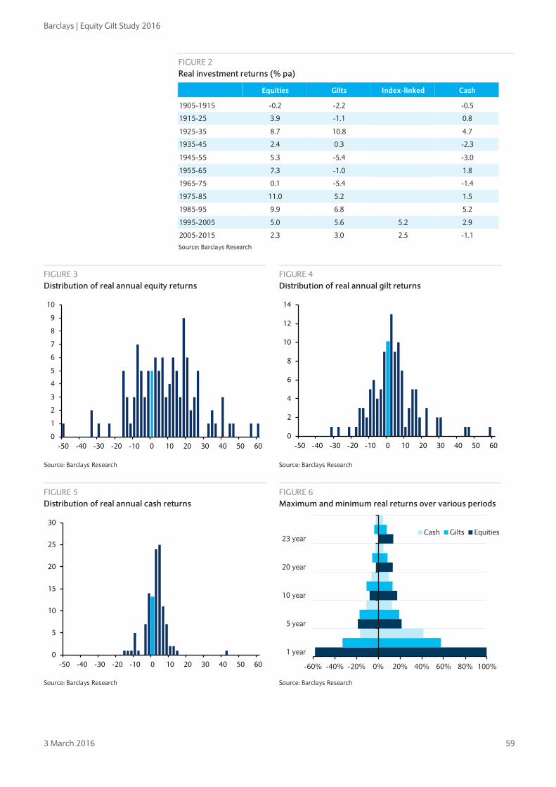
Barclays | Equity Gilt Study 2016
3 March 2016 59
FIGURE 2 Real investment returns (% pa)
Equities Gilts Index-linked Cash
1905-1915 -0.2 -2.2
-0.5
1915-25 3.9 -1.1
0.8
1925-35 8.7 10.8
4.7
1935-45 2.4 0.3
-2.3
1945-55 5.3 -5.4
-3.0
1955-65 7.3 -1.0
1.8
1965-75 0.1 -5.4
-1.4
1975-85 11.0 5.2
1.5
1985-95 9.9 6.8
5.2
1995-2005 5.0 5.6 5.2 2.9
2005-2015 2.3 3.0 2.5 -1.1
Source: Barclays Research
FIGURE 3 Distribution of real annual equity returns
FIGURE 4 Distribution of real annual gilt returns
Source: Barclays Research Source: Barclays Research
FIGURE 5 Distribution of real annual cash returns
FIGURE 6 Maximum and minimum real returns over various periods
Source: Barclays Research Source: Barclays Research
0
1
2
3
4
5
6
7
8
9
10
-50 -40 -30 -20 -10 0 10 20 30 40 50 600
2
4
6
8
10
12
14
-50 -40 -30 -20 -10 0 10 20 30 40 50 60
0
5
10
15
20
25
30
-50 -40 -30 -20 -10 0 10 20 30 40 50 60 -60% -40% -20% 0% 20% 40% 60% 80% 100%
1 year
5 year
10 year
20 year
23 yearCash Gilts Equities
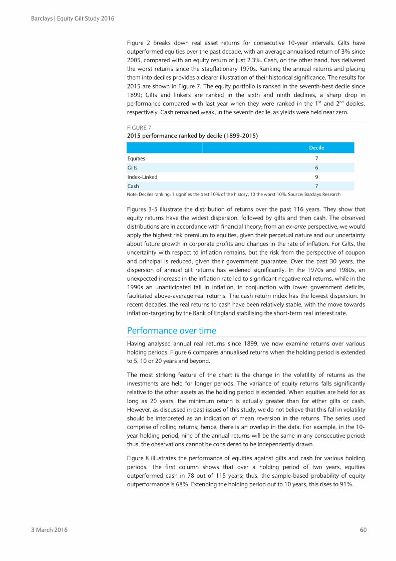
Barclays | Equity Gilt Study 2016
3 March 2016 60
Figure 2 breaks down real asset returns for consecutive 10-year intervals. Gilts have outperformed equities over the past decade, with an average annualised return of 3% since 2005, compared with an equity return of just 2.3%. Cash, on the other hand, has delivered the worst returns since the stagflationary 1970s. Ranking the annual returns and placing them into deciles provides a clearer illustration of their historical significance. The results for 2015 are shown in Figure 7. The equity portfolio is ranked in the seventh-best decile since 1899; Gilts and linkers are ranked in the sixth and ninth declines, a sharp drop in performance compared with last year when they were ranked in the 1st and 2nd deciles, respectively. Cash remained weak, in the seventh decile, as yields were held near zero.
FIGURE 7 2015 performance ranked by decile (1899-2015)
Decile
Equities 7
Gilts 6
Index-Linked 9
Cash 7 Note: Deciles ranking: 1 signifies the best 10% of the history, 10 the worst 10%. Source: Barclays Research
Figures 3-5 illustrate the distribution of returns over the past 116 years. They show that equity returns have the widest dispersion, followed by gilts and then cash. The observed distributions are in accordance with financial theory; from an ex-ante perspective, we would apply the highest risk premium to equities, given their perpetual nature and our uncertainty about future growth in corporate profits and changes in the rate of inflation. For Gilts, the uncertainty with respect to inflation remains, but the risk from the perspective of coupon and principal is reduced, given their government guarantee. Over the past 30 years, the dispersion of annual gilt returns has widened significantly. In the 1970s and 1980s, an unexpected increase in the inflation rate led to significant negative real returns, while in the 1990s an unanticipated fall in inflation, in conjunction with lower government deficits, facilitated above-average real returns. The cash return index has the lowest dispersion. In recent decades, the real returns to cash have been relatively stable, with the move towards inflation-targeting by the Bank of England stabilising the short-term real interest rate.
Performance over time Having analysed annual real returns since 1899, we now examine returns over various holding periods. Figure 6 compares annualised returns when the holding period is extended to 5, 10 or 20 years and beyond.
The most striking feature of the chart is the change in the volatility of returns as the investments are held for longer periods. The variance of equity returns falls significantly relative to the other assets as the holding period is extended. When equities are held for as long as 20 years, the minimum return is actually greater than for either gilts or cash. However, as discussed in past issues of this study, we do not believe that this fall in volatility should be interpreted as an indication of mean reversion in the returns. The series used comprise of rolling returns; hence, there is an overlap in the data. For example, in the 10-year holding period, nine of the annual returns will be the same in any consecutive period; thus, the observations cannot be considered to be independently drawn.
Figure 8 illustrates the performance of equities against gilts and cash for various holding periods. The first column shows that over a holding period of two years, equities outperformed cash in 78 out of 115 years; thus, the sample-based probability of equity outperformance is 68%. Extending the holding period out to 10 years, this rises to 91%.
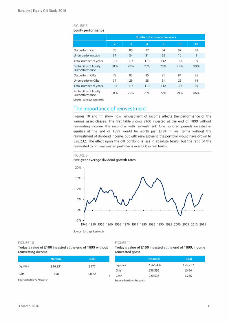
Barclays | Equity Gilt Study 2016
3 March 2016 61
FIGURE 8 Equity performance
Number of consecutive years
2 3 4 5 10 18
Outperform cash 78 80 82 84 97 98
Underperform cash 37 34 31 28 10 1
Total number of years 115 114 113 112 107 99
Probability of Equity Outperformance
68% 70% 73% 75% 91% 99%
Outperform Gilts 78 85 85 81 84 85
Underperform Gilts 37 29 28 31 23 14
Total number of years 115 114 113 112 107 99
Probability of Equity Outperformance 68% 75% 75% 72% 79% 86%
Source: Barclays Research
The importance of reinvestment Figures 10 and 11 show how reinvestment of income affects the performance of the various asset classes. The first table shows £100 invested at the end of 1899 without reinvesting income; the second is with reinvestment. One hundred pounds invested in equities at the end of 1899 would be worth just £184 in real terms without the reinvestment of dividend income, but with reinvestment, the portfolio would have grown to £28,232. The effect upon the gilt portfolio is less in absolute terms, but the ratio of the reinvested to non-reinvested portfolio is over 600 in real terms.
FIGURE 9 Five-year average dividend growth rates
Source: Barclays Research
FIGURE 10 Today’s value of £100 invested at the end of 1899 without reinvesting income
Nominal Real
Equities £14,231 £177 1
Gilts £58 £0.72 0
Source: Barclays Research
FIGURE 11 Today’s value of £100 invested at the end of 1899, income reinvested gross
Nominal Real
Equities £2,265,437 £28,232
Gilts £36,395 £454
Cash £20,535 £256 Source: Barclays Research
-5%
0%
5%
10%
15%
20%
1945 1950 1955 1960 1965 1970 1975 1980 1985 1990 1995 2000 2005 2010 2015
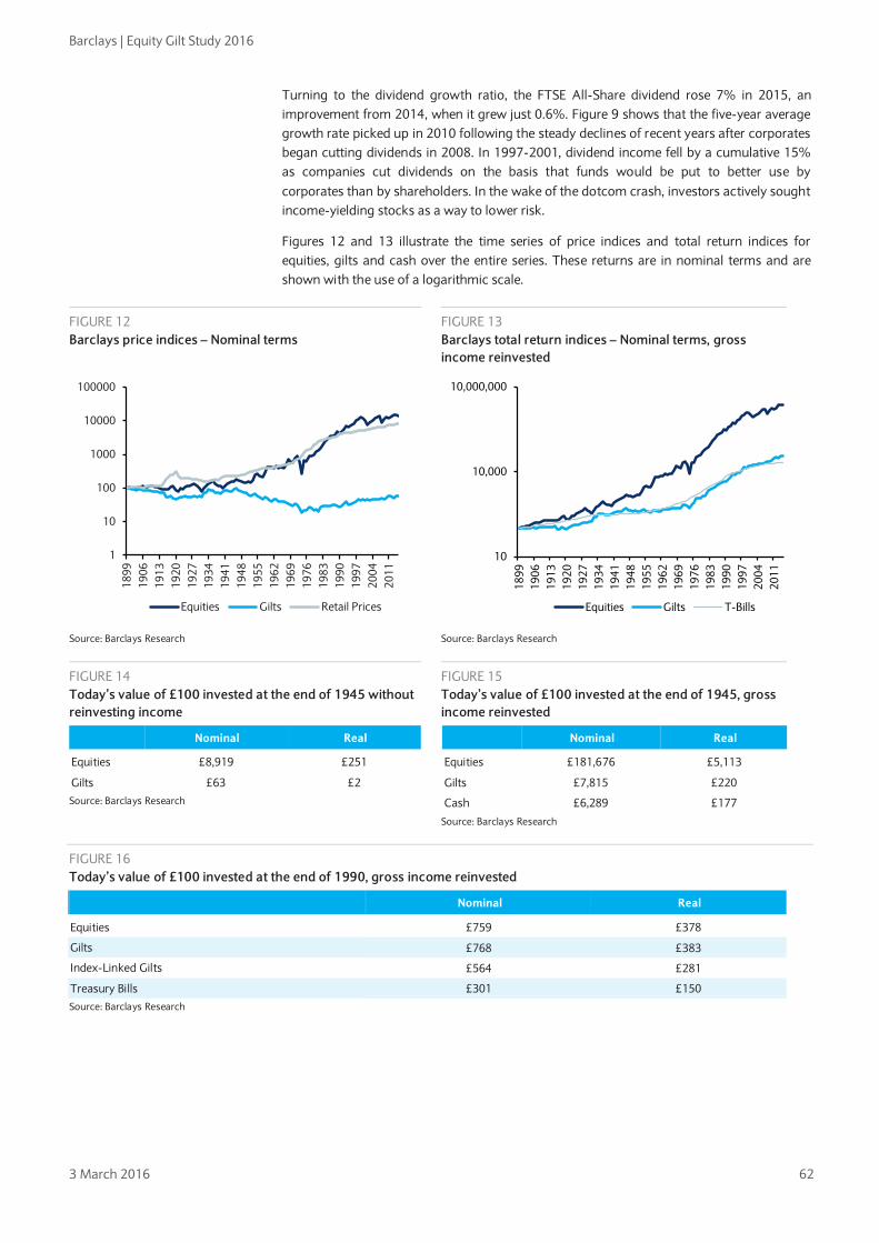
Barclays | Equity Gilt Study 2016
3 March 2016 62
Turning to the dividend growth ratio, the FTSE All-Share dividend rose 7% in 2015, an improvement from 2014, when it grew just 0.6%. Figure 9 shows that the five-year average growth rate picked up in 2010 following the steady declines of recent years after corporates began cutting dividends in 2008. In 1997-2001, dividend income fell by a cumulative 15% as companies cut dividends on the basis that funds would be put to better use by corporates than by shareholders. In the wake of the dotcom crash, investors actively sought income-yielding stocks as a way to lower risk.
Figures 12 and 13 illustrate the time series of price indices and total return indices for equities, gilts and cash over the entire series. These returns are in nominal terms and are shown with the use of a logarithmic scale.
FIGURE 12 Barclays price indices – Nominal terms
FIGURE 13 Barclays total return indices – Nominal terms, gross income reinvested
Source: Barclays Research Source: Barclays Research
FIGURE 14 Today’s value of £100 invested at the end of 1945 without reinvesting income
Nominal Real
Equities £8,919 £251
Gilts £63 £2 Source: Barclays Research
FIGURE 15 Today’s value of £100 invested at the end of 1945, gross income reinvested
Nominal Real
Equities £181,676 £5,113
Gilts £7,815 £220
Cash £6,289 £177
Source: Barclays Research
FIGURE 16 Today’s value of £100 invested at the end of 1990, gross income reinvested
Nominal Real
Equities £759 £378
Gilts £768 £383
Index-Linked Gilts £564 £281
Treasury Bills £301 £150 Source: Barclays Research
1
10
100
1000
10000
100000
1899
1906
1913
1920
1927
1934
1941
1948
1955
1962
1969
1976
1983
1990
1997
2004
2011
Equities Gilts Retail Prices
10
10,000
10,000,000
1899
1906
1913
1920
1927
1934
1941
1948
1955
1962
1969
1976
1983
1990
1997
2004
2011
Equities Gilts T-Bills

Barclays | Equity Gilt Study 2016
3 March 2016 63
CHAPTER 6
US asset returns since 1925 We analyse returns on equities, government bonds and cash. The total sample includes 90 annual return observations. The construction of the series is explained in more detail in Chapter 7 (“Barclays Indices”). The corporate bond performance is captured using the Barclays Investment Grade Corporate Long Index, which incorporates bonds with a maturity of 10 years or more. The Barclays US Inflation Linked 15-year Plus Index is used to represent the performance of TIPS. The nominal return series are deflated by the change in the consumer price index, which is calculated by the Bureau of Labor Statistics. The first holding period covered in this analysis is the calendar year 1926, representing money invested at the end of 1925 and its value at the end of 1926.
FIGURE 1 Real investment returns (% pa)
Last 2015 10 years 20 years 50 years 90 years*
Equities -2.4 4.9 5.8 5.3 6.6
Government Bond -1.2 4.6 4.8 3.4 2.6
TIPS -8.7 2.9
Corporate Bond -5.3 4.2 4.4
Cash -0.7 -0.7 0.2 0.8 0.5
Inflation 0.7 1.9 2.2 4.1 2.9 Note: * Entire sample. Source: Centre for Research into Security Prices (CRSP), Barclays Research
Figure 1 provides real annualized returns over various time horizons. 2015 was a difficult year for US assets, with negative real returns across the board. The US growth backdrop weakened relative to 2014, while actual and expected inflation trended lower. Oil continued to play a key role in driving asset prices, and the Fed finally tightened monetary policy in December following months of speculation. US equity returns collapsed relative to 2014. Real total returns were just -2.4% in 2015, in contrast to 9.7% the prior year. US 2015 growth expectations were steadily downgraded over the year. Expectations for real GDP had started the year close to 3% y/y before being derated gradually to close to 2% y/y as activity data in the first half of the year proved weaker than initially expected. Global shocks, such as the China yuan depreciation, actually hit European equities harder initially given the greater exposure to Asian trade. However, European equities still managed to outperform US and UK over the year as the ECB’s announcement of QE in January provided European stocks with a headstart.
Fixed income markets followed the trends in the UK: nominal bond real returns collapsed from 23% in 2014 to -1.2% in 2015, while inflation-linked bonds were the worst-performing asset in the US as well as the UK. Weak 2015 returns dragged the 10-year annualised average return for TIPS sharply lower, from 4% last year to 2.9%. Investment grade corporate credit returns were almost as poor as in 2008 and 2013 in nominal terms. US credit markets faced a number of headwinds last year. Increased M&A-related issuance weighed on returns, while the decline in commodity prices led to underperformance of the investment grade energy credits as investors feared downgrades.
Sreekala Kochugovindan +44 (0)20 7773 2234 sreekala.kochugovindan@ barclays.com Barclays, UK

Barclays | Equity Gilt Study 2016
3 March 2016 64
FIGURE 2 Real investment returns (% pa)
Equities Government Bond Corporate Bond Cash
1925-35 6.7 7.7
4.6
1935-45 6.0 1.6
-2.6
1945-55 10.6 -2.4
-2.7
1955-65 9.5 0.0
1.0
1965-75 -2.8 -2.5
-0.1
1975-85 8.0 2.2
2.0
1985-95 10.1 7.9 7.7 2.0
1995-2005 6.6 5.0 4.6 1.0
2005-15 4.9 4.6 4.2 -0.7
Source: CRSP, Barclays Research
Equities outperformed Treasuries and corporate bonds in the most recent decade. A total real return of 4.9% is far below the average performance since 1925 of 6.6%. Equities’ best decades were in the immediate aftermath of World War Two and the 1980s. Bonds have enjoyed strong performance over the past three decades relative to preceding decades, largely as a result of continued disinflation since the late 1970s. Figure 2 highlights that the interwar decade 1925-35 also proved to be a good decade for government bonds.
Figure 3 ranks the relative performance of 2015 returns by deciles to get a clearer indication of their historical significance. The US equity ranking has fallen from the 6th decile in 2014 to the 8th decile in 2015 as performance faltered. Bonds moved from the best decile in 2014 to the 7th decile in 2015 as investors focused on the timing of the Fed’s first policy rate hike in over a decade. Cash returns remained weak, with negative real returns placing them in the 7th decile.
FIGURE 3 Comparison of 2013 real returns with historical performance ranked by decile
Decile
Equities 8
Govt Bond 7
Cash 7 Note: Deciles ranking - 1 signifies the best 10% of the history, 10 the worst 10%. Source: CRSP, Barclays Research
Figures 4-6 plot the sample distributions with identical maximum and minimum categories across each. These charts are useful in that they allow the reader to appreciate the volatility of each asset class while gaining an understanding of the distribution of the annual return observations. Clearly, overall, cash exhibits the lowest volatility of each asset class, with bonds next and equities having the highest dispersion of returns.

Barclays | Equity Gilt Study 2016
3 March 2016 65
FIGURE 4 Distribution of real annual cash returns
FIGURE 5 Distribution of real annual bond returns
Source: CRSP, Barclays Research Source: CRSP, Barclays Research
FIGURE 6 Distribution of real annual equity returns
FIGURE 7 Maximum and minimum real returns over different periods
Source: CRSP, Barclays Research Source: CRSP, Barclays Research
Figure 7 shows the extremes of the return distribution for various holding periods. The volatility of equities over very short horizons is clearly demonstrated in the maximum and minimum distribution of one-year returns. As we extend the holding period, the distribution begins to narrow. Over the past 90 years, the worst average annualised 20-year return for equities was 0.9%, while the best was 13%. However, this is not to say that it is impossible to lose money by holding equities over a 20-year period, as the analysis is conducted on an ex-post basis. The figure merely highlights that such an occurrence seems unlikely, given equities’ performance over the past 90 years.
In addition, over the long term, we would expect the ex-ante equity risk premium to provide a cushion against uncertainty. Bonds and cash have experienced negative returns over a 20-year investment horizon, reflecting unexpected jumps in inflation at various points in the past century.
Figure 8 plots the US equity risk premium and shows that the 10-year annualized excess return of equities over bonds has recovered from the lows of 2008 and remains only slightly in positive territory at 0.3%.
0
5
10
15
20
25
30
35
-50 -40 -30 -20 -10 0 10 20 30 40 50 600
2
4
6
8
10
12
-50 -40 -30 -20 -10 0 10 20 30 40 50 60
0
1
2
3
4
5
6
7
-50 -40 -30 -20 -10 0 10 20 30 40 50 60-50% -30% -10% 10% 30% 50%
1 year
5 year
10 year
20 yearCash Bonds Equities
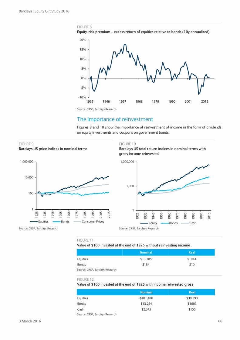
Barclays | Equity Gilt Study 2016
3 March 2016 66
FIGURE 8 Equity-risk premium – excess return of equities relative to bonds (10y annualized)
Source: CRSP, Barclays Research
The importance of reinvestment Figures 9 and 10 show the importance of reinvestment of income in the form of dividends on equity investments and coupons on government bonds.
FIGURE 11 Value of $100 invested at the end of 1925 without reinvesting income
Nominal Real
Equities $13,785 $1044
Bonds $134 $10
Source: CRSP, Barclays Research
FIGURE 12 Value of $100 invested at the end of 1925 with income reinvested gross
Nominal Real
Equities $401,488 $30,393
Bonds $13,254 $1003
Cash $2,043 $155 Source: CRSP, Barclays Research
-10%
-5%
0%
5%
10%
15%
20%
1935 1946 1957 1968 1979 1990 2001 2012
FIGURE 9 Barclays US price indices in nominal terms
FIGURE 10 Barclays US total return indices in nominal terms with gross income reinvested
Source: CRSP, Barclays Research Source: CRSP, Barclays Research
1
100
10,000
1,000,000
1925
1935
1945
1955
1965
1975
1985
1995
2005
2015
Equities Bonds Consumer Prices
1
1,000
1,000,000
1925
1935
1945
1955
1965
1975
1985
1995
2005
2015
Equity Bonds Cash

Barclays | Equity Gilt Study 2016
3 March 2016 67
CHAPTER 7
Barclays indices We have calculated three indices showing: 1) changes in the capital value of each asset class; 2) changes to income from these investments; and 3) a combined measure of the overall return, on the assumption that all income is reinvested.
Additional series allow for the effects of inflation. The data for cash include building society deposit rates and Treasury bills. The series on index-linked securities is based at December 1982 and the corporate bond index starts at the end of 1990.
Barclays Equity Index The Barclays Equity Index is designed to give as accurate a measure as possible of the performance of a representative portfolio of equities. Three main types of index can be used. The FT Index, which for years was the most widely used in the UK, is geometric, meaning that the price changes of the 30 shares it comprises are multiplied together to produce the change in the index. We believe that this is a fair basis for indicating short-term market behaviour, but that over long periods it imparts a downward bias. The second type of index uses the Dow formula, in which the prices of a number of shares are added together. This does not have the distorting effect of a geometric index, but the weighting of the various shares is arbitrary and varies with changes in capitalisation.
We think the most accurate and representative indices are arithmetic and weighted by the number of shares in issue by each company. These indices include virtually all of the large quoted companies, and thus we believe they accurately reflect the behaviour of an equity market. The Standard & Poor’s Indices are of this type, and they date back to the 1920s. The FT Actuaries Indices, introduced in the 1960s, were the first of this type in the UK. Subsequently, a number of weighted arithmetic international indices, such as those calculated by Morgan Stanley Capital International and Datastream, have been introduced. More recently, the FTSE 100 Index, which uses the same construction but incorporates only the 100 leading shares, has been introduced and, generally, is now used as the main market indicator because it is calculated on a real-time basis throughout the day.
The Barclays Equity Index, which is used in this study, is a weighted arithmetic index, and is available for the period since 1899, with a dividend yield and an income index. The original Barclays Equity Index, used in editions of this study until 1999, was first calculated retrospectively in 1956 and included 30 shares chosen because of their similarities to the FT 30 Index, which covers the 1935 to 1962 period. For the 2000 edition of this study, we compiled a new index for 1899-1935, based on the 30 largest shares by market capitalisation in each year. From 1962, the Barclays Equity Index is based on the FTSE Actuaries All-Share Index because, with its broader coverage, it gives a more accurate picture of market movements. The indices are calculated only annually, at year-end.
The equity returns between 1899 and 1935 are therefore calculated from a new Equity Index, consisting of the 30 largest shares by market capitalisation in each year; between 1935 and 1962 they are calculated from the FT 30 Index and from 1962 onward they are derived from the FTSE Actuaries All-Share Index.
Sreekala Kochugovindan +44 (0)20 7773 2234 sreekala.kochugovindan@ barclays.com Barclays, UK

Barclays | Equity Gilt Study 2016
3 March 2016 68
FIGURE 1 Equity Index constituents
Constituents at December 1899 Constituents at December 1934 Constituents at December 1962
De Beers Consolidated Mines Rio Tinto Ltd Armstrong Whitworth Consolidated Gold Fields London and County Bank
Woolworth Ltd Imperial Chemical Industries Shell' Transport & Trading Ltd Courtaulds Ltd Royal Insurance Co
Associated Portland Cement Bass Mitchells & Butlers British Motor Coats Patons Cory (William)
London City & Midland Bank Ltd Lloyds Bank Ltd London & Westminster Bank Ltd Vickers, Sons & Maxim Ltd Imperial Ottoman Bank
Barclay & Company Lloyds Bank Prudential Assurance Co Ltd Westminster Bank Ltd Midland Bank Ltd
Courtaulds Distillers Dunlop EMI Fine Spinners & Doublers
Parrs Bank Ltd Royal Insurance Co Tharsis Sulphur & Copper Ltd Great Northern of Copenhagen Simmer & Jack PropietaryMines Ltd
London & Lancashire Fire Ins. Co North British & Mercantile In. Co Ltd Reckitt & Sons Ltd County of London Electric Supply Co Unilever Ltd
General Electric Guest Keen Hawker Siddeley House of Fraser ICI
North British & Mercantile Insurance Consett Iron Ltd Eastern Extension Australasia * China Ltd Nobel Dynamite TstLtd Mysore Gold Mining Ltd
Tate & Lyle Ltd Alliance Assurance Company Boots Pure Drug Co Ltd Pearl Assurance Co Marks & Spencer Ltd
Imperial Tobacco International Stores Leyland Motors London Brick Murex
Exploration Co Alliance Assurance Co Aerated Bread Ltd Howard & Bullough Ltd Sun Insurance Office
Cory (WM.) & Son National Bank Of Egypt Consolidated Gold Fields Of South Africa Bass, Ratcliff & Gretton Ltd GeduldProp Mines Ltd
P&O Steam Navigation Rolls-Royce Swan Hunter Tate & Lyle Tube Investments
New JagersfonteinMining & Expl Ltd Champion Reef Gold Mining National Telephone Ltd Northern Assurance Phoenix Assurance Co
Sun Insurance Office Bank Of Australasia British South Africa Co Chartered Bank Of India, Australia & China North Eastern Elec Supply Co
Turner & Newall United Steel Vickers WatneyMann Woolworth
Source: Barclays Research
The Equity Index is a weighted arithmetic average. In the Equity Index, the weights of the 30 constituent companies for each year are proportional to their market capitalisation at the beginning of the year. Each year a fund was constructed. The number of shares in the fund for each company was calculated so that its market value at the beginning of the year was equal to the company’s index weighting. The value of the fund was calculated annually at the end of the year.
For 1899-1962, the Equity Income Index is based on the Barclays Equity Fund. The Income Index relates to the dividend income actually received in the 12 months prior to the date of the index. It is calculated by totalling the dividends paid on the shares in the fund. We believe that it is the only published index based on actual income receipts.
From 1963 the Income Index is derived from the yield on the FTSE All-Share Index. Despite a minimal discontinuity in the yield, in our view, this is the most representative method of evaluating equity performance over the period. The dividend yield is quoted net from 1998, with non-taxpayers no longer able to reclaim ACT.
Barclays Gilt Index The Gilt Index measures the performance of long-dated gilts. From 1899 to 1962 the index is based on the prices of undated British funds. During this period the undated stocks were a major part of the gilt market, but over the years the effect of high interest rates on their

Barclays | Equity Gilt Study 2016
3 March 2016 69
prices, together with the growing number of conventional long-dated issues, meant that undated stocks became less and less representative of the market as a whole.
Since 1962, the Barclays Gilt Index has been based on a portfolio of long-dated stocks, selected on 1 January each year. The portfolio was chosen to represent as closely as possible a 20-year security on a par yield, and contains a weighted combination of four long-dated stocks with a mean life of 20½ years (so that the average life of the stocks for the year in which they are in the portfolio was 20 years). The combination and weightings of the four stocks are chosen to have the minimum possible deviation from a par yield. Small issues (less than £1bn) are excluded and in any year none of the four stocks has been allocated a weight of more than 40%, or less than 5% of the index.
During the late 1980s there was a steady contraction in the number of issues that satisfied the criteria for inclusion in the Gilt Index. As a result of the lack of issues of new long-dated stocks and the fall in the remaining life of existing stocks, the universe of eligible stocks narrowed sharply. By the end of 1989 there were four stocks with a life of more than 20 years, and only two of these were over £1bn nominal.
Thus from the beginning of 1990 the index has been constructed to represent a portfolio of 15-year par yielding gilts.
Barclays Inflation-linked Index The index-linked market has now been established for almost three decades and is capitalised at £530bn (compared with the £1.3trn capitalisation of the conventional market). The index has been constructed to mirror as closely as possible the rules of the conventional gilt index. An average life of 20 years was used up until 1990, and 15 years thereafter. Again, stocks have been chosen to be as close to par as possible, although of course in this case par means “indexed par”.
Barclays Corporate Bond Index The UK corporate bond market has expanded markedly since the beginning of 1999. The index and returns are based on the Barclays Sterling Aggregate Corporate Index. Clearly, we are unable to select individual stocks for this index in the way we do for the gilt indices because such a small sample of stocks cannot be representative of the market.
Barclays Building Society Fund In previous editions of this study we have included indices of the value of £100 invested in a building society at the end of 1945. We originally used the average interest rate on an ordinary share account. In the mid-1980s many building societies introduced new tiered interest rate accounts, which provided a higher rate of interest while still allowing instant access. In response to this we have been tracking both types of account, but as time progressed the old style “ordinary share accounts” became less and less representative and by the mid-1990s had been completely superseded by the new accounts. From 1986 the Barclays Index follows the Halifax Liquid Gold Account (formerly called the Halifax Instant Xtra) as a representative of the newer tiered interest rate-style accounts. The Halifax is no longer a building society, having converted to a bank, so from 1998 we follow the Nationwide Invest Direct Account. This is the closest equivalent account offered by the Nationwide Building Society (which is now the largest remaining building society in the UK); the difference is that it is operated by post. We consider this type of postal account to be more representative of building society returns than the branch operated passbook accounts, which are more in the nature of a cash-based transaction account.
US asset returns The US indices used in this study were provided by the Center for Research in Security Prices (CRSP) at the Graduate School of Business of the University of Chicago. The value-

Barclays | Equity Gilt Study 2016
3 March 2016 70
weighted equity index covers all common stocks trading on the New York, Nasdaq, and Arca Stock Exchanges, excluding ADRs. For the bond index, the CRSP has used software which selects the bond that is closest to a 20-year bond in each month. The same methodology has been employed for the 30-day T-Bill.
Total returns In this study, we have shown the performance of representative investments in UK equities and long gilts, with additional analysis of equivalent US returns in both monetary and real (inflation adjusted) terms. The total returns to the investor, however, also include the income on the investment. This is important throughout the study for comparability between asset classes. For example, when constructing an index for a cash investment such as the UK Treasury Bill Index, the £100 invested at the end of 1899 grew to approximately £104 by the end of the following year. This full amount is reinvested and by the end of 1920 the value of this investment had grown to about £190. In contrast, equity and bond market returns can be split into two components: capital appreciation; and dividend income. The most commonly quoted stock market indices usually include only the capital component of the return. In order to calculate returns on a comparable basis, we need to include the returns obtained by reinvesting this income. This is particularly important in looking at bonds where the scope for capital appreciation is small, so almost all of the return will be from income. In this study, total returns are calculated assuming income is reinvested at the end of the year.
Taxation The total return to an investor depends crucially on the tax regime. The largest long-term investors in the British equity and gilt markets are pension funds and similar institutions that (until the abolition of the advance corporation tax (ACT) credit) have not suffered tax on their income or capital; our main tables therefore make no allowance for tax until 1998, which was the first full year that non-taxpayers were unable to reclaim the ACT credit. This effectively reduced the dividend yield to non-taxpayers, and is reflected in our main tables and gross total return series.
The personal investor must suffer tax. The net return to a building society account is straightforward to compute. However, changes in the tax regime in recent years make the net return to equity and gilt investment less straightforward to calculate on a consistent basis. For example, the change to total return taxation for gilts means that it is inappropriate to calculate a net total return on the basis of taxing income alone. Thus returns are quoted gross throughout, but for reference we also quote basic tax rates.
Arithmetic and geometric averages Our analysis of past data usually relies on calculations of the geometric mean for each series. Arithmetic averages can provide a misleading picture. For example, suppose equities rose from a base of 100 to 200 over one year and then fell back to 100 over the next year. The return for year one would have been 100% and for year two minus 50%. The arithmetic average return would be 25% even though equities are actually unchanged in value over the two years.
The geometric average return in this example would be zero. This method of calculation is therefore preferable. Over long periods, the geometric average for total returns is the rate at which a sum invested at the beginning of the period will grow to by the end of the period, assuming all income is reinvested. The calculation of geometric averages depends only on the initial and final values for the investment, not particular values at any other point in time.
For periods of one year, arithmetic and geometric averages will be the same. But over longer periods the geometric average is always less than the arithmetic average, except when all the individual yearly returns are the same. For the mathematically minded, the geometric return is approximately equal to the arithmetic return minus one-half the variance of the arithmetic return.

Barclays | Equity Gilt Study 2016
3 March 2016 71
Although geometric returns are appropriate to analyse the past, arithmetic returns should be used to provide forecasts. Arithmetic averages provide the better unbiased estimator of returns (for a statistical proof of this see Ian Cooper’s paper Arithmetic vs Geometric Premium: setting discount rates for capital budgeting calculations, IFA Working Paper 174-93, April 1993).
Capital value indices The indices in Figure 2 show the nominal capital value of £100 invested in equities and gilts at the end of 1899. The chart also plots the Barclays Cost of Living Index. Note how the equity index has correlated with increases in the cost of living versus a similar investment in gilts. The index values at the end of 2015 were 14,231 for equities, 57.6 for gilts, and 8024 for the cost of living.
We then show the same capital indices adjusted for the increase in the cost of living since 1899. Figure 3 shows the end-2015 real equity price index at 177 with the real gilt price index at 0.72.
Total return indices The next two charts show the nominal and real value of the equity, gilt and cash funds with gross income received reinvested at the end of each year since 1899. Figure 4 shows that the nominal worth of £100 invested in equities at the end of 1899 was £2,265,437. The same investment in gilts was worth £36,395 and in T-Bills £20,535. When adjusted for inflation, the equity fund is worth £28,232, the gilt £454 and the cash fund £256.

Barclays | Equity Gilt Study 2016
3 March 2016 72
FIGURE 2 Barclays price indices in nominal terms
FIGURE 3 Barclays price indices in real terms
Source: Barclays Research Source: Barclays Research
FIGURE 4 Barclays total return indices in nominal terms with gross income reinvested
FIGURE 5 Barclays total return indices in real terms with gross income reinvested
Source: Barclays Research Source: Barclays Research
1
10
100
1,000
10,000
100,000
1899 1913 1927 1941 1955 1969 1983 1997 2011
Equities Gilts Retail prices
0
50
100
150
200
250
300
1899 1911 1923 1935 1947 1959 1971 1983 1995 2007
Equities Gilts
1
10
100
1,000
10,000
100,000
1,000,000
10,000,000
1899 1913 1927 1941 1955 1969 1983 1997 2011
Equities Gilts T-Bills
1
10
100
1,000
10,000
100,000
1899 1913 1927 1941 1955 1969 1983 1997 2011
Equities Gilts T- Bills
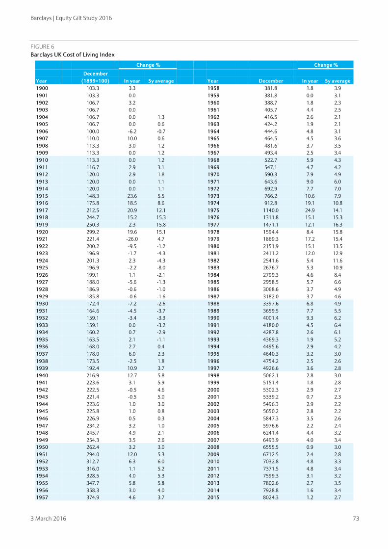
Barclays | Equity Gilt Study 2016
3 March 2016 73
FIGURE 6 Barclays UK Cost of Living Index
Change % Change %
Year December
(1899=100) In year 5y average Year December In year 5y average 1900 103.3 3.3 1958 381.8 1.8 3.9 1901 103.3 0.0 1959 381.8 0.0 3.1 1902 106.7 3.2 1960 388.7 1.8 2.3 1903 106.7 0.0 1961 405.7 4.4 2.5 1904 106.7 0.0 1.3 1962 416.5 2.6 2.1 1905 106.7 0.0 0.6 1963 424.2 1.9 2.1 1906 100.0 -6.2 -0.7 1964 444.6 4.8 3.1 1907 110.0 10.0 0.6 1965 464.5 4.5 3.6 1908 113.3 3.0 1.2 1966 481.6 3.7 3.5 1909 113.3 0.0 1.2 1967 493.4 2.5 3.4 1910 113.3 0.0 1.2 1968 522.7 5.9 4.3 1911 116.7 2.9 3.1 1969 547.1 4.7 4.2 1912 120.0 2.9 1.8 1970 590.3 7.9 4.9 1913 120.0 0.0 1.1 1971 643.6 9.0 6.0 1914 120.0 0.0 1.1 1972 692.9 7.7 7.0 1915 148.3 23.6 5.5 1973 766.2 10.6 7.9 1916 175.8 18.5 8.6 1974 912.8 19.1 10.8 1917 212.5 20.9 12.1 1975 1140.0 24.9 14.1 1918 244.7 15.2 15.3 1976 1311.8 15.1 15.3 1919 250.3 2.3 15.8 1977 1471.1 12.1 16.3 1920 299.2 19.6 15.1 1978 1594.4 8.4 15.8 1921 221.4 -26.0 4.7 1979 1869.3 17.2 15.4 1922 200.2 -9.5 -1.2 1980 2151.9 15.1 13.5 1923 196.9 -1.7 -4.3 1981 2411.2 12.0 12.9 1924 201.3 2.3 -4.3 1982 2541.6 5.4 11.6 1925 196.9 -2.2 -8.0 1983 2676.7 5.3 10.9 1926 199.1 1.1 -2.1 1984 2799.3 4.6 8.4 1927 188.0 -5.6 -1.3 1985 2958.5 5.7 6.6 1928 186.9 -0.6 -1.0 1986 3068.6 3.7 4.9 1929 185.8 -0.6 -1.6 1987 3182.0 3.7 4.6 1930 172.4 -7.2 -2.6 1988 3397.6 6.8 4.9 1931 164.6 -4.5 -3.7 1989 3659.5 7.7 5.5 1932 159.1 -3.4 -3.3 1990 4001.4 9.3 6.2 1933 159.1 0.0 -3.2 1991 4180.0 4.5 6.4 1934 160.2 0.7 -2.9 1992 4287.8 2.6 6.1 1935 163.5 2.1 -1.1 1993 4369.3 1.9 5.2 1936 168.0 2.7 0.4 1994 4495.6 2.9 4.2 1937 178.0 6.0 2.3 1995 4640.3 3.2 3.0 1938 173.5 -2.5 1.8 1996 4754.2 2.5 2.6 1939 192.4 10.9 3.7 1997 4926.6 3.6 2.8 1940 216.9 12.7 5.8 1998 5062.1 2.8 3.0 1941 223.6 3.1 5.9 1999 5151.4 1.8 2.8 1942 222.5 -0.5 4.6 2000 5302.3 2.9 2.7 1943 221.4 -0.5 5.0 2001 5339.2 0.7 2.3 1944 223.6 1.0 3.0 2002 5496.3 2.9 2.2 1945 225.8 1.0 0.8 2003 5650.2 2.8 2.2 1946 226.9 0.5 0.3 2004 5847.3 3.5 2.6 1947 234.2 3.2 1.0 2005 5976.6 2.2 2.4 1948 245.7 4.9 2.1 2006 6241.4 4.4 3.2 1949 254.3 3.5 2.6 2007 6493.9 4.0 3.4 1950 262.4 3.2 3.0 2008 6555.5 0.9 3.0 1951 294.0 12.0 5.3 2009 6712.5 2.4 2.8 1952 312.7 6.3 6.0 2010 7032.8 4.8 3.3 1953 316.0 1.1 5.2 2011 7371.5 4.8 3.4 1954 328.5 4.0 5.3 2012 7599.3 3.1 3.2 1955 347.7 5.8 5.8 2013 7802.6 2.7 3.5 1956 358.3 3.0 4.0 2014 7928.8 1.6 3.4 1957 374.9 4.6 3.7 2015 8024.3 1.2 2.7
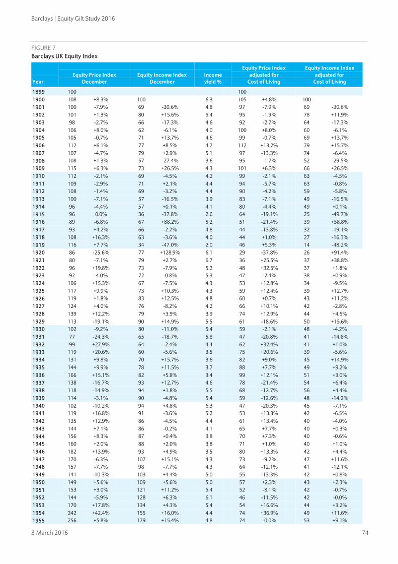
Barclays | Equity Gilt Study 2016
3 March 2016 74
FIGURE 7 Barclays UK Equity Index
Year Equity Price Index
December Equity Income Index
December Income yield %
Equity Price Index adjusted for
Cost of Living
Equity Income Index adjusted for
Cost of Living
1899 100 100 1900 108 +8.3% 100 6.3 105 +4.8% 100 1901 100 -7.9% 69 -30.6% 4.8 97 -7.9% 69 -30.6% 1902 101 +1.3% 80 +15.6% 5.4 95 -1.9% 78 +11.9% 1903 98 -2.7% 66 -17.3% 4.6 92 -2.7% 64 -17.3% 1904 106 +8.0% 62 -6.1% 4.0 100 +8.0% 60 -6.1% 1905 105 -0.7% 71 +13.7% 4.6 99 -0.7% 69 +13.7% 1906 112 +6.1% 77 +8.5% 4.7 112 +13.2% 79 +15.7% 1907 107 -4.7% 79 +2.9% 5.1 97 -13.3% 74 -6.4% 1908 108 +1.3% 57 -27.4% 3.6 95 -1.7% 52 -29.5% 1909 115 +6.3% 73 +26.5% 4.3 101 +6.3% 66 +26.5% 1910 112 -2.1% 69 -4.5% 4.2 99 -2.1% 63 -4.5% 1911 109 -2.9% 71 +2.1% 4.4 94 -5.7% 63 -0.8% 1912 108 -1.4% 69 -3.2% 4.4 90 -4.2% 59 -5.8% 1913 100 -7.1% 57 -16.5% 3.9 83 -7.1% 49 -16.5% 1914 96 -4.4% 57 +0.1% 4.1 80 -4.4% 49 +0.1% 1915 96 0.0% 36 -37.8% 2.6 64 -19.1% 25 -49.7% 1916 89 -6.8% 67 +88.2% 5.2 51 -21.4% 39 +58.8% 1917 93 +4.2% 66 -2.2% 4.8 44 -13.8% 32 -19.1% 1918 108 +16.3% 63 -3.6% 4.0 44 +1.0% 27 -16.3% 1919 116 +7.7% 34 -47.0% 2.0 46 +5.3% 14 -48.2% 1920 86 -25.6% 77 +128.9% 6.1 29 -37.8% 26 +91.4% 1921 80 -7.1% 79 +2.7% 6.7 36 +25.5% 37 +38.8% 1922 96 +19.8% 73 -7.9% 5.2 48 +32.5% 37 +1.8% 1923 92 -4.0% 72 -0.8% 5.3 47 -2.4% 38 +0.9% 1924 106 +15.3% 67 -7.5% 4.3 53 +12.8% 34 -9.5% 1925 117 +9.9% 73 +10.3% 4.3 59 +12.4% 39 +12.7% 1926 119 +1.8% 83 +12.5% 4.8 60 +0.7% 43 +11.2% 1927 124 +4.0% 76 -8.2% 4.2 66 +10.1% 42 -2.8% 1928 139 +12.2% 79 +3.9% 3.9 74 +12.9% 44 +4.5% 1929 113 -19.1% 90 +14.9% 5.5 61 -18.6% 50 +15.6% 1930 102 -9.2% 80 -11.0% 5.4 59 -2.1% 48 -4.2% 1931 77 -24.3% 65 -18.7% 5.8 47 -20.8% 41 -14.8% 1932 99 +27.9% 64 -2.4% 4.4 62 +32.4% 41 +1.0% 1933 119 +20.6% 60 -5.6% 3.5 75 +20.6% 39 -5.6% 1934 131 +9.8% 70 +15.7% 3.6 82 +9.0% 45 +14.9% 1935 144 +9.9% 78 +11.5% 3.7 88 +7.7% 49 +9.2% 1936 166 +15.1% 82 +5.8% 3.4 99 +12.1% 51 +3.0% 1937 138 -16.7% 93 +12.7% 4.6 78 -21.4% 54 +6.4% 1938 118 -14.9% 94 +1.8% 5.5 68 -12.7% 56 +4.4% 1939 114 -3.1% 90 -4.8% 5.4 59 -12.6% 48 -14.2% 1940 102 -10.2% 94 +4.8% 6.3 47 -20.3% 45 -7.1% 1941 119 +16.8% 91 -3.6% 5.2 53 +13.3% 42 -6.5% 1942 135 +12.9% 86 -4.5% 4.4 61 +13.4% 40 -4.0% 1943 144 +7.1% 86 -0.2% 4.1 65 +7.7% 40 +0.3% 1944 156 +8.3% 87 +0.4% 3.8 70 +7.3% 40 -0.6% 1945 160 +2.0% 88 +2.0% 3.8 71 +1.0% 40 +1.0% 1946 182 +13.9% 93 +4.9% 3.5 80 +13.3% 42 +4.4% 1947 170 -6.3% 107 +15.1% 4.3 73 -9.2% 47 +11.6% 1948 157 -7.7% 98 -7.7% 4.3 64 -12.1% 41 -12.1% 1949 141 -10.3% 103 +4.4% 5.0 55 -13.3% 42 +0.8% 1950 149 +5.6% 109 +5.6% 5.0 57 +2.3% 43 +2.3% 1951 153 +3.0% 121 +11.2% 5.4 52 -8.1% 42 -0.7% 1952 144 -5.9% 128 +6.3% 6.1 46 -11.5% 42 -0.0% 1953 170 +17.8% 134 +4.3% 5.4 54 +16.6% 44 +3.2% 1954 242 +42.4% 155 +16.0% 4.4 74 +36.9% 49 +11.6% 1955 256 +5.8% 179 +15.4% 4.8 74 -0.0% 53 +9.1%
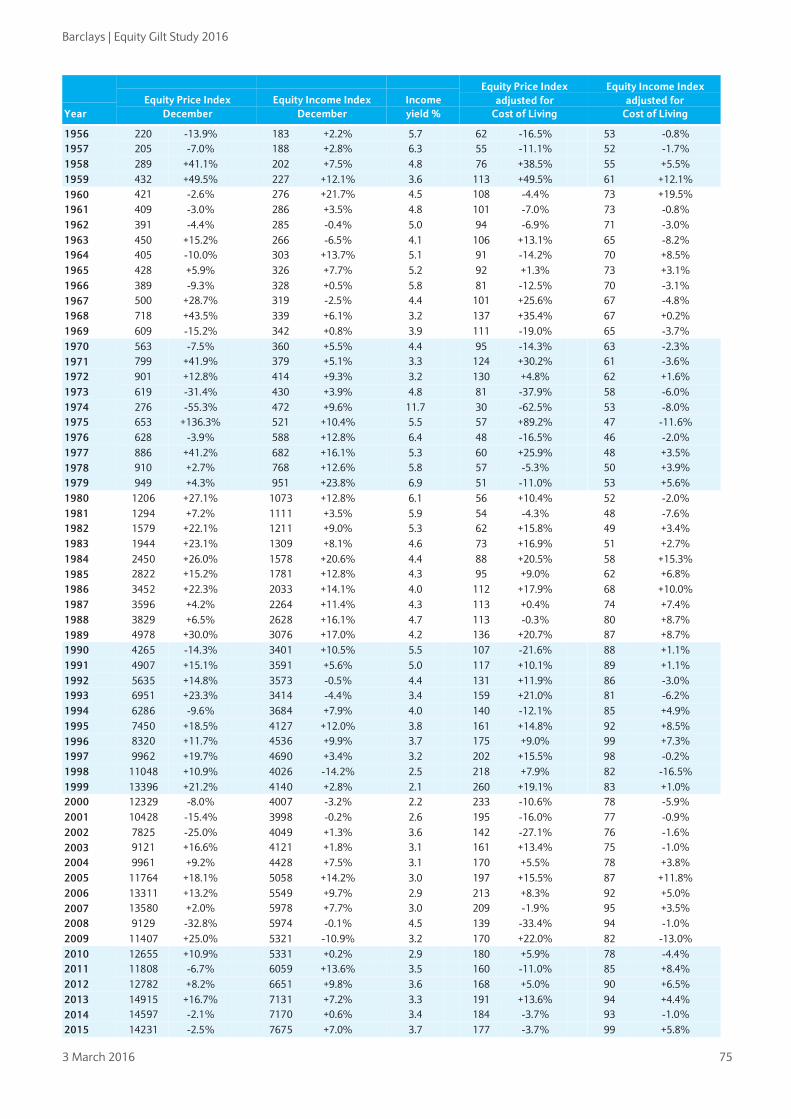
Barclays | Equity Gilt Study 2016
3 March 2016 75
Year Equity Price Index
December Equity Income Index
December Income yield %
Equity Price Index adjusted for
Cost of Living
Equity Income Index adjusted for
Cost of Living
1956 220 -13.9% 183 +2.2% 5.7 62 -16.5% 53 -0.8% 1957 205 -7.0% 188 +2.8% 6.3 55 -11.1% 52 -1.7% 1958 289 +41.1% 202 +7.5% 4.8 76 +38.5% 55 +5.5% 1959 432 +49.5% 227 +12.1% 3.6 113 +49.5% 61 +12.1% 1960 421 -2.6% 276 +21.7% 4.5 108 -4.4% 73 +19.5% 1961 409 -3.0% 286 +3.5% 4.8 101 -7.0% 73 -0.8% 1962 391 -4.4% 285 -0.4% 5.0 94 -6.9% 71 -3.0% 1963 450 +15.2% 266 -6.5% 4.1 106 +13.1% 65 -8.2% 1964 405 -10.0% 303 +13.7% 5.1 91 -14.2% 70 +8.5% 1965 428 +5.9% 326 +7.7% 5.2 92 +1.3% 73 +3.1% 1966 389 -9.3% 328 +0.5% 5.8 81 -12.5% 70 -3.1% 1967 500 +28.7% 319 -2.5% 4.4 101 +25.6% 67 -4.8% 1968 718 +43.5% 339 +6.1% 3.2 137 +35.4% 67 +0.2% 1969 609 -15.2% 342 +0.8% 3.9 111 -19.0% 65 -3.7% 1970 563 -7.5% 360 +5.5% 4.4 95 -14.3% 63 -2.3% 1971 799 +41.9% 379 +5.1% 3.3 124 +30.2% 61 -3.6% 1972 901 +12.8% 414 +9.3% 3.2 130 +4.8% 62 +1.6% 1973 619 -31.4% 430 +3.9% 4.8 81 -37.9% 58 -6.0% 1974 276 -55.3% 472 +9.6% 11.7 30 -62.5% 53 -8.0% 1975 653 +136.3% 521 +10.4% 5.5 57 +89.2% 47 -11.6% 1976 628 -3.9% 588 +12.8% 6.4 48 -16.5% 46 -2.0% 1977 886 +41.2% 682 +16.1% 5.3 60 +25.9% 48 +3.5% 1978 910 +2.7% 768 +12.6% 5.8 57 -5.3% 50 +3.9% 1979 949 +4.3% 951 +23.8% 6.9 51 -11.0% 53 +5.6% 1980 1206 +27.1% 1073 +12.8% 6.1 56 +10.4% 52 -2.0% 1981 1294 +7.2% 1111 +3.5% 5.9 54 -4.3% 48 -7.6% 1982 1579 +22.1% 1211 +9.0% 5.3 62 +15.8% 49 +3.4% 1983 1944 +23.1% 1309 +8.1% 4.6 73 +16.9% 51 +2.7% 1984 2450 +26.0% 1578 +20.6% 4.4 88 +20.5% 58 +15.3% 1985 2822 +15.2% 1781 +12.8% 4.3 95 +9.0% 62 +6.8% 1986 3452 +22.3% 2033 +14.1% 4.0 112 +17.9% 68 +10.0% 1987 3596 +4.2% 2264 +11.4% 4.3 113 +0.4% 74 +7.4% 1988 3829 +6.5% 2628 +16.1% 4.7 113 -0.3% 80 +8.7% 1989 4978 +30.0% 3076 +17.0% 4.2 136 +20.7% 87 +8.7% 1990 4265 -14.3% 3401 +10.5% 5.5 107 -21.6% 88 +1.1% 1991 4907 +15.1% 3591 +5.6% 5.0 117 +10.1% 89 +1.1% 1992 5635 +14.8% 3573 -0.5% 4.4 131 +11.9% 86 -3.0% 1993 6951 +23.3% 3414 -4.4% 3.4 159 +21.0% 81 -6.2% 1994 6286 -9.6% 3684 +7.9% 4.0 140 -12.1% 85 +4.9% 1995 7450 +18.5% 4127 +12.0% 3.8 161 +14.8% 92 +8.5% 1996 8320 +11.7% 4536 +9.9% 3.7 175 +9.0% 99 +7.3% 1997 9962 +19.7% 4690 +3.4% 3.2 202 +15.5% 98 -0.2% 1998 11048 +10.9% 4026 -14.2% 2.5 218 +7.9% 82 -16.5% 1999 13396 +21.2% 4140 +2.8% 2.1 260 +19.1% 83 +1.0% 2000 12329 -8.0% 4007 -3.2% 2.2 233 -10.6% 78 -5.9% 2001 10428 -15.4% 3998 -0.2% 2.6 195 -16.0% 77 -0.9% 2002 7825 -25.0% 4049 +1.3% 3.6 142 -27.1% 76 -1.6% 2003 9121 +16.6% 4121 +1.8% 3.1 161 +13.4% 75 -1.0% 2004 9961 +9.2% 4428 +7.5% 3.1 170 +5.5% 78 +3.8% 2005 11764 +18.1% 5058 +14.2% 3.0 197 +15.5% 87 +11.8% 2006 13311 +13.2% 5549 +9.7% 2.9 213 +8.3% 92 +5.0% 2007 13580 +2.0% 5978 +7.7% 3.0 209 -1.9% 95 +3.5% 2008 9129 -32.8% 5974 -0.1% 4.5 139 -33.4% 94 -1.0% 2009 11407 +25.0% 5321 -10.9% 3.2 170 +22.0% 82 -13.0% 2010 12655 +10.9% 5331 +0.2% 2.9 180 +5.9% 78 -4.4% 2011 11808 -6.7% 6059 +13.6% 3.5 160 -11.0% 85 +8.4% 2012 12782 +8.2% 6651 +9.8% 3.6 168 +5.0% 90 +6.5% 2013 14915 +16.7% 7131 +7.2% 3.3 191 +13.6% 94 +4.4% 2014 14597 -2.1% 7170 +0.6% 3.4 184 -3.7% 93 -1.0% 2015 14231 -2.5% 7675 +7.0% 3.7 177 -3.7% 99 +5.8%

Barclays | Equity Gilt Study 2016
3 March 2016 76
FIGURE 8 Barclays UK Gilt Index
Year Gilt Price Index
December Yield % Gilt Price Index
Adjusted for Cost of Living
1899 100.0 100.0 1900 98.4 -1.6% 2.8 95.2 -4.8% 1901 94.6 -3.8% 2.9 91.5 -3.8% 1902 93.7 -0.9% 3.0 87.8 -4.0% 1903 88.3 -5.8% 2.9 82.8 -5.8% 1904 89.4 +1.2% 2.8 83.8 +1.2% 1905 90.1 +0.8% 2.8 84.4 +0.8% 1906 86.6 -3.8% 2.9 86.6 +2.6% 1907 84.1 -2.9% 3.0 76.5 -11.7% 1908 84.6 +0.6% 3.0 74.7 -2.4% 1909 83.6 -1.3% 3.0 73.7 -1.3% 1910 80.0 -4.3% 3.1 70.6 -4.3% 1911 77.7 -2.8% 3.2 66.6 -5.6% 1912 75.8 -2.4% 3.3 63.2 -5.1% 1913 72.3 -4.7% 3.5 60.2 -4.7% 1914 73.0 +1.0% 3.4 60.9 +1.0% 1915 73.0 0.0 3.4 49.2 -19.1% 1916 55.7 -23.8% 4.5 31.7 -35.7% 1917 54.9 -1.4% 4.6 25.8 -18.4% 1918 59.4 +8.3% 4.2 24.3 -6.0% 1919 51.9 -12.7% 4.8 20.7 -14.6% 1920 45.6 -12.1% 5.5 15.2 -26.5% 1921 50.6 +11.1% 4.9 22.9 +50.2% 1922 56.2 +10.9% 4.4 28.1 +22.6% 1923 56.1 -0.2% 4.5 28.5 +1.5% 1924 57.7 +2.9% 4.3 28.6 +0.6% 1925 55.4 -3.9% 4.5 28.1 -1.7% 1926 54.5 -1.6% 4.6 27.4 -2.7% 1927 55.9 +2.6% 4.5 29.8 +8.7% 1928 56.7 +1.3% 4.4 30.3 +1.9% 1929 53.3 -6.0% 4.7 28.7 -5.4% 1930 57.8 +8.5% 4.3 33.5 +16.9% 1931 55.0 -4.7% 4.5 33.4 -0.2% 1932 74.7 +35.6% 3.3 46.9 +40.4% 1933 74.6 -0.1% 3.3 46.9 -0.1% 1934 92.8 +24.4% 2.7 57.9 +23.5% 1935 87.4 -5.8% 2.9 53.4 -7.8% 1936 85.1 -2.6% 2.9 50.7 -5.2% 1937 74.8 -12.2% 3.3 42.0 -17.1% 1938 70.7 -5.4% 3.5 40.8 -3.0% 1939 68.9 -2.6% 3.6 35.8 -12.2% 1940 77.4 +12.3% 3.2 35.7 -0.3% 1941 83.1 +7.4% 3.0 37.2 +4.2% 1942 82.9 -0.3% 3.0 37.2 +0.2% 1943 80.0 -3.4% 3.1 36.1 -3.0% 1944 82.1 +2.6% 3.0 36.7 +1.6% 1945 91.8 +11.8% 2.7 40.6 +10.7% 1946 99.2 +8.0% 2.5 43.7 +7.5% 1947 82.5 -16.8% 3.0 35.2 -19.4% 1948 80.6 -2.3% 3.1 32.8 -6.9% 1949 70.9 -12.0% 3.5 27.9 -15.0% 1950 71.3 +0.5% 3.5 27.2 -2.6% 1951 61.9 -13.1% 4.0 21.1 -22.4% 1952 59.0 -4.8% 4.2 18.9 -10.5% 1953 64.7 +9.7% 3.9 20.5 +8.5% 1954 66.1 +2.2% 3.8 20.1 -1.7% 1955 56.9 -13.8% 4.4 16.4 -18.6%

Barclays | Equity Gilt Study 2016
3 March 2016 77
Year Gilt Price Index
December Yield % Gilt Price Index
Adjusted for Cost of Living
1956 52.7 -7.5% 4.7 14.7 -10.2% 1957 46.9 -10.9% 5.3 12.5 -14.9% 1958 52.4 +11.7% 4.8 13.7 +9.6% 1959 50.4 -3.9% 5.0 13.2 -3.9% 1960 44.3 -11.9% 5.6 11.4 -13.5% 1961 38.3 -13.7% 6.5 9.4 -17.3% 1962 45.3 +18.3% 5.4 10.9 +15.3% 1963 44.5 -1.7% 5.5 10.5 -3.5% 1964 41.0 -7.9% 6.1 9.2 -12.1% 1965 40.3 -1.7% 6.2 8.7 -6.0% 1966 39.5 -2.1% 6.4 8.2 -5.5% 1967 37.9 -4.1% 6.9 7.7 -6.4% 1968 34.4 -9.3% 7.6 6.6 -14.4% 1969 31.7 -7.6% 8.5 5.8 -11.7% 1970 30.1 -5.2% 9.3 5.1 -12.2% 1971 35.4 +17.6% 8.3 5.5 +7.8% 1972 31.0 -12.3% 9.6 4.5 -18.5% 1973 25.3 -18.6% 11.9 3.3 -26.4% 1974 18.3 -27.5% 17.0 2.0 -39.2% 1975 21.8 +19.2% 14.8 1.9 -4.6% 1976 21.6 -1.1% 15.0 1.6 -14.0% 1977 28.2 +30.6% 10.9 1.9 +16.4% 1978 24.4 -13.3% 13.2 1.5 -20.0% 1979 22.2 -9.2% 14.7 1.2 -22.6% 1980 23.5 +6.2% 13.9 1.1 -7.8% 1981 20.7 -12.1% 15.8 0.9 -21.6% 1982 28.2 +36.2% 11.1 1.1 +29.2% 1983 29.5 +4.9% 10.5 1.1 -0.4% 1984 28.5 -3.4% 10.6 1.0 -7.7% 1985 28.7 +0.4% 10.5 1.0 -5.0% 1986 28.8 +0.4% 10.5 0.9 -3.2% 1987 30.6 +6.2% 9.5 1.0 +2.4% 1988 30.6 +0.0% 9.3 0.9 -6.3% 1989 29.4 -3.7% 10.0 0.8 -10.6% 1990 28.1 -4.5% 10.6 0.7 -12.7% 1991 30.4 +8.0% 9.8 0.7 +3.4% 1992 33.0 +8.7% 8.7 0.8 +6.0% 1993 39.4 +19.3% 6.4 0.9 +17.1% 1994 32.2 -18.1% 8.6 0.7 -20.4% 1995 35.5 +10.3% 7.6 0.8 +6.8% 1996 35.7 +0.6% 7.6 0.8 -1.8% 1997 40.0 +11.8% 6.3 0.8 +7.9% 1998 47.4 +18.6% 4.4 0.9 +15.4% 1999 43.4 -8.4% 5.3 0.8 -10.0% 2000 45.2 +4.0% 4.7 0.9 +1.0% 2001 43.4 -3.8% 5.0 0.8 -4.5% 2002 45.5 +4.8% 4.4 0.8 +1.8% 2003 44.1 -3.2% 4.7 0.8 -5.8% 2004 45.2 +2.5% 4.5 0.8 -1.0% 2005 47.0 +3.9% 4.1 0.8 +1.7% 2006 44.8 -4.6% 4.7 0.7 -8.6% 2007 45.1 +0.6% 4.5 0.7 -3.3% 2008 48.8 +8.3% 3.4 0.7 +7.3% 2009 46.4 -5.0% 4.2 0.7 -7.3% 2010 48.7 +5.0% 3.6 0.7 +0.3% 2011 57.2 +17.4% 2.4 0.8 +12.0% 2012 57.9 +1.3% 2.2 0.8 -1.7% 2013 51.8 -10.6% 3.3 0.7 -12.9% 2014 59.3 +14.4% 2.1 0.7 +12.6% 2015 57.6 -2.8% 2.3 0.7 -4.0%

Barclays | Equity Gilt Study 2016
3 March 2016 78
FIGURE 9 Barclays UK Treasury Bill Index
Year Treasury Bill Index
December Treasury Bill Index
adjusted for cost of living
1899 100 100 1900 104 +4.0% 101 +0.6% 1901 107 +2.5% 103 +2.5% 1902 110 +3.0% 103 -0.3% 1903 114 +3.4% 106 +3.4% 1904 117 +2.9% 110 +2.9% 1905 119 +2.2% 112 +2.2% 1906 123 +3.0% 123 +9.9% 1907 128 +3.8% 116 -5.7% 1908 130 +2.2% 115 -0.8% 1909 133 +2.1% 118 +2.1% 1910 137 +3.1% 121 +3.1% 1911 141 +2.8% 121 -0.1% 1912 144 +2.0% 120 -0.8% 1913 148 +3.0% 124 +3.0% 1914 153 +3.0% 127 +3.0% 1915 158 +3.0% 106 -16.6% 1916 162 +3.0% 92 -13.1% 1917 167 +3.0% 79 -14.7% 1918 172 +3.0% 70 -10.5% 1919 179 +3.6% 71 +1.3% 1920 190 +6.5% 64 -11.0% 1921 199 +4.7% 90 +41.5% 1922 204 +2.6% 102 +13.4% 1923 210 +2.7% 107 +4.4% 1924 217 +3.5% 108 +1.2% 1925 226 +4.2% 115 +6.6% 1926 237 +4.6% 119 +3.5% 1927 247 +4.4% 131 +10.5% 1928 257 +4.3% 138 +4.9% 1929 271 +5.4% 146 +6.1% 1930 278 +2.5% 161 +10.5% 1931 289 +3.7% 175 +8.6% 1932 293 +1.5% 184 +5.0% 1933 295 +0.6% 185 +0.6% 1934 297 +0.7% 185 +0.0% 1935 298 +0.5% 182 -1.5% 1936 300 +0.6% 179 -2.1% 1937 302 +0.6% 170 -5.1% 1938 304 +0.6% 175 +3.2% 1939 308 +1.3% 160 -8.6% 1940 311 +1.0% 143 -10.4% 1941 314 +1.0% 140 -2.0% 1942 317 +2.0% 143 +1.5% 1943 320 +1.0% 145 +1.5% 1944 324 +1.0% 145 +0.0% 1945 327 +0.9% 145 -0.1% 1946 328 +0.5% 145 +0.0% 1947 330 +0.5% 141 -2.6% 1948 332 +0.5% 135 -4.2% 1949 333 +0.5% 131 -2.9% 1950 335 +0.5% 128 -2.6% 1951 337 +0.5% 115 -10.3% 1952 344 +2.1% 110 -4.0% 1953 352 +2.4% 111 +1.3% 1954 359 +1.9% 109 -2.0% 1955 371 +3.5% 107 -2.2%
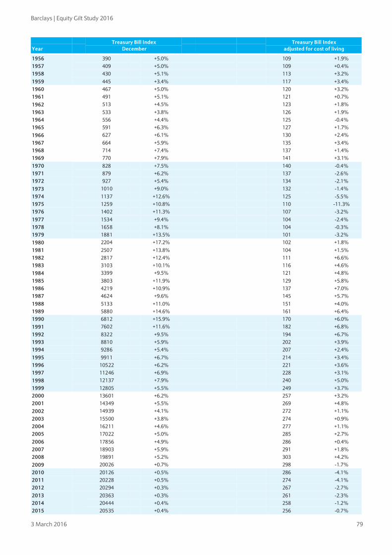
Barclays | Equity Gilt Study 2016
3 March 2016 79
Year Treasury Bill Index
December Treasury Bill Index
adjusted for cost of living
1956 390 +5.0% 109 +1.9% 1957 409 +5.0% 109 +0.4% 1958 430 +5.1% 113 +3.2% 1959 445 +3.4% 117 +3.4% 1960 467 +5.0% 120 +3.2% 1961 491 +5.1% 121 +0.7% 1962 513 +4.5% 123 +1.8% 1963 533 +3.8% 126 +1.9% 1964 556 +4.4% 125 -0.4% 1965 591 +6.3% 127 +1.7% 1966 627 +6.1% 130 +2.4% 1967 664 +5.9% 135 +3.4% 1968 714 +7.4% 137 +1.4% 1969 770 +7.9% 141 +3.1% 1970 828 +7.5% 140 -0.4% 1971 879 +6.2% 137 -2.6% 1972 927 +5.4% 134 -2.1% 1973 1010 +9.0% 132 -1.4% 1974 1137 +12.6% 125 -5.5% 1975 1259 +10.8% 110 -11.3% 1976 1402 +11.3% 107 -3.2% 1977 1534 +9.4% 104 -2.4% 1978 1658 +8.1% 104 -0.3% 1979 1881 +13.5% 101 -3.2% 1980 2204 +17.2% 102 +1.8% 1981 2507 +13.8% 104 +1.5% 1982 2817 +12.4% 111 +6.6% 1983 3103 +10.1% 116 +4.6% 1984 3399 +9.5% 121 +4.8% 1985 3803 +11.9% 129 +5.8% 1986 4219 +10.9% 137 +7.0% 1987 4624 +9.6% 145 +5.7% 1988 5133 +11.0% 151 +4.0% 1989 5880 +14.6% 161 +6.4% 1990 6812 +15.9% 170 +6.0% 1991 7602 +11.6% 182 +6.8% 1992 8322 +9.5% 194 +6.7% 1993 8810 +5.9% 202 +3.9% 1994 9286 +5.4% 207 +2.4% 1995 9911 +6.7% 214 +3.4% 1996 10522 +6.2% 221 +3.6% 1997 11246 +6.9% 228 +3.1% 1998 12137 +7.9% 240 +5.0% 1999 12805 +5.5% 249 +3.7% 2000 13601 +6.2% 257 +3.2% 2001 14349 +5.5% 269 +4.8% 2002 14939 +4.1% 272 +1.1% 2003 15500 +3.8% 274 +0.9% 2004 16211 +4.6% 277 +1.1% 2005 17022 +5.0% 285 +2.7% 2006 17856 +4.9% 286 +0.4% 2007 18903 +5.9% 291 +1.8% 2008 19891 +5.2% 303 +4.2% 2009 20026 +0.7% 298 -1.7% 2010 20126 +0.5% 286 -4.1% 2011 20228 +0.5% 274 -4.1% 2012 20294 +0.3% 267 -2.7% 2013 20363 +0.3% 261 -2.3% 2014 20444 +0.4% 258 -1.2% 2015 20535 +0.4% 256 -0.7%
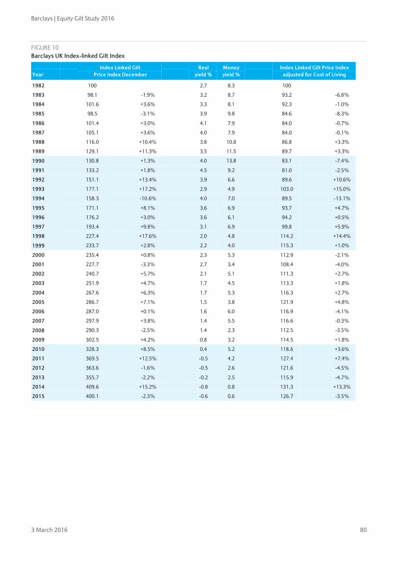
Barclays | Equity Gilt Study 2016
3 March 2016 80
FIGURE 10 Barclays UK Index-linked Gilt Index
Year Index Linked Gilt
Price Index December Real
yield % Money yield %
Index Linked Gilt Price Index adjusted for Cost of Living
1982 100 2.7 8.3 100
1983 98.1 -1.9% 3.2 8.7 93.2 -6.8%
1984 101.6 +3.6% 3.3 8.1 92.3 -1.0%
1985 98.5 -3.1% 3.9 9.8 84.6 -8.3%
1986 101.4 +3.0% 4.1 7.9 84.0 -0.7%
1987 105.1 +3.6% 4.0 7.9 84.0 -0.1%
1988 116.0 +10.4% 3.8 10.8 86.8 +3.3%
1989 129.1 +11.3% 3.5 11.5 89.7 +3.3%
1990 130.8 +1.3% 4.0 13.8 83.1 -7.4%
1991 133.2 +1.8% 4.5 9.2 81.0 -2.5%
1992 151.1 +13.4% 3.9 6.6 89.6 +10.6%
1993 177.1 +17.2% 2.9 4.9 103.0 +15.0%
1994 158.3 -10.6% 4.0 7.0 89.5 -13.1%
1995 171.1 +8.1% 3.6 6.9 93.7 +4.7%
1996 176.2 +3.0% 3.6 6.1 94.2 +0.5%
1997 193.4 +9.8% 3.1 6.9 99.8 +5.9%
1998 227.4 +17.6% 2.0 4.8 114.2 +14.4%
1999 233.7 +2.8% 2.2 4.0 115.3 +1.0%
2000 235.4 +0.8% 2.3 5.3 112.9 -2.1%
2001 227.7 -3.3% 2.7 3.4 108.4 -4.0%
2002 240.7 +5.7% 2.1 5.1 111.3 +2.7%
2003 251.9 +4.7% 1.7 4.5 113.3 +1.8%
2004 267.6 +6.3% 1.7 5.3 116.3 +2.7%
2005 286.7 +7.1% 1.5 3.8 121.9 +4.8%
2006 287.0 +0.1% 1.6 6.0 116.9 -4.1%
2007 297.9 +3.8% 1.4 5.5 116.6 -0.3%
2008 290.3 -2.5% 1.4 2.3 112.5 -3.5%
2009 302.5 +4.2% 0.8 3.2 114.5 +1.8%
2010 328.3 +8.5% 0.4 5.2 118.6 +3.6%
2011 369.5 +12.5% -0.5 4.2 127.4 +7.4%
2012 363.6 -1.6% -0.5 2.6 121.6 -4.5%
2013 355.7 -2.2% -0.2 2.5 115.9 -4.7%
2014 409.6 +15.2% -0.8 0.8 131.3 +13.3%
2015 400.1 -2.3% -0.6 0.6 126.7 -3.5%
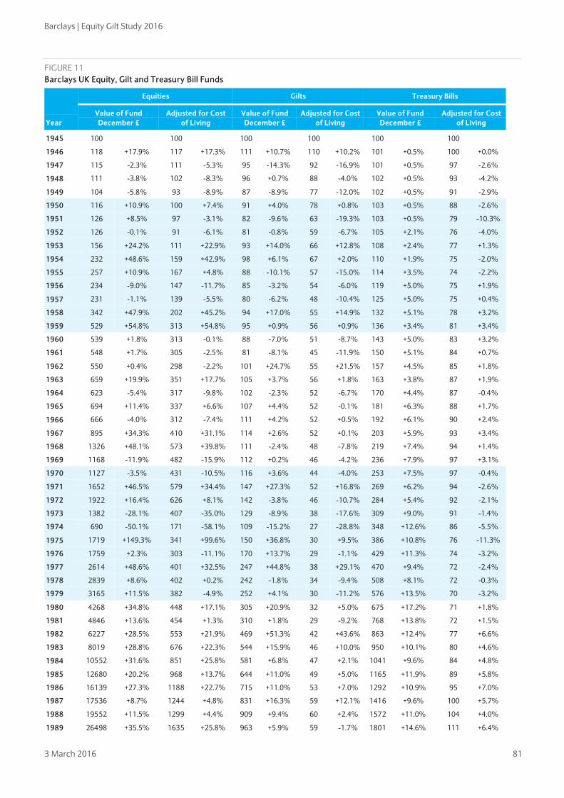
Barclays | Equity Gilt Study 2016
3 March 2016 81
FIGURE 11 Barclays UK Equity, Gilt and Treasury Bill Funds
Year
Equities Gilts Treasury Bills
Value of Fund December £
Adjusted for Cost of Living
Value of Fund December £
Adjusted for Cost of Living
Value of Fund December £
Adjusted for Cost of Living
1945 100 100 100 100 100 100
1946 118 +17.9% 117 +17.3% 111 +10.7% 110 +10.2% 101 +0.5% 100 +0.0%
1947 115 -2.3% 111 -5.3% 95 -14.3% 92 -16.9% 101 +0.5% 97 -2.6%
1948 111 -3.8% 102 -8.3% 96 +0.7% 88 -4.0% 102 +0.5% 93 -4.2%
1949 104 -5.8% 93 -8.9% 87 -8.9% 77 -12.0% 102 +0.5% 91 -2.9%
1950 116 +10.9% 100 +7.4% 91 +4.0% 78 +0.8% 103 +0.5% 88 -2.6%
1951 126 +8.5% 97 -3.1% 82 -9.6% 63 -19.3% 103 +0.5% 79 -10.3%
1952 126 -0.1% 91 -6.1% 81 -0.8% 59 -6.7% 105 +2.1% 76 -4.0%
1953 156 +24.2% 111 +22.9% 93 +14.0% 66 +12.8% 108 +2.4% 77 +1.3%
1954 232 +48.6% 159 +42.9% 98 +6.1% 67 +2.0% 110 +1.9% 75 -2.0%
1955 257 +10.9% 167 +4.8% 88 -10.1% 57 -15.0% 114 +3.5% 74 -2.2%
1956 234 -9.0% 147 -11.7% 85 -3.2% 54 -6.0% 119 +5.0% 75 +1.9%
1957 231 -1.1% 139 -5.5% 80 -6.2% 48 -10.4% 125 +5.0% 75 +0.4%
1958 342 +47.9% 202 +45.2% 94 +17.0% 55 +14.9% 132 +5.1% 78 +3.2%
1959 529 +54.8% 313 +54.8% 95 +0.9% 56 +0.9% 136 +3.4% 81 +3.4%
1960 539 +1.8% 313 -0.1% 88 -7.0% 51 -8.7% 143 +5.0% 83 +3.2%
1961 548 +1.7% 305 -2.5% 81 -8.1% 45 -11.9% 150 +5.1% 84 +0.7%
1962 550 +0.4% 298 -2.2% 101 +24.7% 55 +21.5% 157 +4.5% 85 +1.8%
1963 659 +19.9% 351 +17.7% 105 +3.7% 56 +1.8% 163 +3.8% 87 +1.9%
1964 623 -5.4% 317 -9.8% 102 -2.3% 52 -6.7% 170 +4.4% 87 -0.4%
1965 694 +11.4% 337 +6.6% 107 +4.4% 52 -0.1% 181 +6.3% 88 +1.7%
1966 666 -4.0% 312 -7.4% 111 +4.2% 52 +0.5% 192 +6.1% 90 +2.4%
1967 895 +34.3% 410 +31.1% 114 +2.6% 52 +0.1% 203 +5.9% 93 +3.4%
1968 1326 +48.1% 573 +39.8% 111 -2.4% 48 -7.8% 219 +7.4% 94 +1.4%
1969 1168 -11.9% 482 -15.9% 112 +0.2% 46 -4.2% 236 +7.9% 97 +3.1%
1970 1127 -3.5% 431 -10.5% 116 +3.6% 44 -4.0% 253 +7.5% 97 -0.4%
1971 1652 +46.5% 579 +34.4% 147 +27.3% 52 +16.8% 269 +6.2% 94 -2.6%
1972 1922 +16.4% 626 +8.1% 142 -3.8% 46 -10.7% 284 +5.4% 92 -2.1%
1973 1382 -28.1% 407 -35.0% 129 -8.9% 38 -17.6% 309 +9.0% 91 -1.4%
1974 690 -50.1% 171 -58.1% 109 -15.2% 27 -28.8% 348 +12.6% 86 -5.5%
1975 1719 +149.3% 341 +99.6% 150 +36.8% 30 +9.5% 386 +10.8% 76 -11.3%
1976 1759 +2.3% 303 -11.1% 170 +13.7% 29 -1.1% 429 +11.3% 74 -3.2%
1977 2614 +48.6% 401 +32.5% 247 +44.8% 38 +29.1% 470 +9.4% 72 -2.4%
1978 2839 +8.6% 402 +0.2% 242 -1.8% 34 -9.4% 508 +8.1% 72 -0.3%
1979 3165 +11.5% 382 -4.9% 252 +4.1% 30 -11.2% 576 +13.5% 70 -3.2%
1980 4268 +34.8% 448 +17.1% 305 +20.9% 32 +5.0% 675 +17.2% 71 +1.8%
1981 4846 +13.6% 454 +1.3% 310 +1.8% 29 -9.2% 768 +13.8% 72 +1.5%
1982 6227 +28.5% 553 +21.9% 469 +51.3% 42 +43.6% 863 +12.4% 77 +6.6%
1983 8019 +28.8% 676 +22.3% 544 +15.9% 46 +10.0% 950 +10.1% 80 +4.6%
1984 10552 +31.6% 851 +25.8% 581 +6.8% 47 +2.1% 1041 +9.6% 84 +4.8%
1985 12680 +20.2% 968 +13.7% 644 +11.0% 49 +5.0% 1165 +11.9% 89 +5.8%
1986 16139 +27.3% 1188 +22.7% 715 +11.0% 53 +7.0% 1292 +10.9% 95 +7.0%
1987 17536 +8.7% 1244 +4.8% 831 +16.3% 59 +12.1% 1416 +9.6% 100 +5.7%
1988 19552 +11.5% 1299 +4.4% 909 +9.4% 60 +2.4% 1572 +11.0% 104 +4.0%
1989 26498 +35.5% 1635 +25.8% 963 +5.9% 59 -1.7% 1801 +14.6% 111 +6.4%

Barclays | Equity Gilt Study 2016
3 March 2016 82
Year
Equities Gilts Treasury Bills
Value of Fund December £
Adjusted for Cost of Living
Value of Fund December £
Adjusted for Cost of Living
Value of Fund December £
Adjusted for Cost of Living
1990 23947 -9.6% 1351 -17.4% 1017 +5.6% 57 -3.4% 2086 +15.9% 118 +6.0%
1991 28936 +20.8% 1563 +15.7% 1209 +18.9% 65 +13.8% 2328 +11.6% 126 +6.8%
1992 34672 +19.8% 1826 +16.8% 1432 +18.4% 75 +15.4% 2549 +9.5% 134 +6.7%
1993 44207 +27.5% 2285 +25.1% 1844 +28.8% 95 +26.4% 2698 +5.9% 139 +3.9%
1994 41590 -5.9% 2089 -8.6% 1635 -11.3% 82 -13.8% 2844 +5.4% 143 +2.4%
1995 51163 +23.0% 2490 +19.2% 1945 +19.0% 95 +15.3% 3035 +6.7% 148 +3.4%
1996 59275 +15.9% 2815 +13.1% 2095 +7.7% 100 +5.1% 3222 +6.2% 153 +3.6%
1997 73263 +23.6% 3358 +19.3% 2503 +19.4% 115 +15.3% 3444 +6.9% 158 +3.1%
1998 83284 +13.7% 3715 +10.6% 3129 +25.0% 140 +21.7% 3717 +7.9% 166 +5.0%
1999 103120 +23.8% 4520 +21.7% 3018 -3.5% 132 -5.2% 3921 +5.5% 172 +3.7%
2000 97023 -5.9% 4132 -8.6% 3296 +9.2% 140 +6.1% 4165 +6.2% 177 +3.2%
2001 84226 -13.2% 3562 -13.8% 3340 +1.3% 141 +0.6% 4394 +5.5% 186 +4.8%
2002 65440 -22.3% 2689 -24.5% 3668 +9.8% 151 +6.7% 4575 +4.1% 188 +1.1%
2003 78643 +20.2% 3143 +16.9% 3725 +1.6% 149 -1.2% 4747 +3.8% 190 +0.9%
2004 88508 +12.5% 3418 +8.8% 3994 +7.2% 154 +3.6% 4964 +4.6% 192 +1.1%
2005 107609 +21.6% 4066 +18.9% 4329 +8.4% 164 +6.0% 5213 +5.0% 197 +2.7%
2006 125243 +16.4% 4531 +11.4% 4323 -0.1% 156 -4.4% 5468 +4.9% 198 +0.4%
2007 131639 +5.1% 4577 +1.0% 4550 +5.2% 158 +1.2% 5789 +5.9% 201 +1.8%
2008 92460 -29.8% 3185 -30.4% 5135 +12.9% 177 +11.8% 6091 +5.2% 210 +4.2%
2009 119238 +29.0% 4011 +25.9% 5087 -1.0% 171 -3.3% 6133 +0.7% 206 -1.7%
2010 136107 +14.1% 4370 +8.9% 5565 +9.4% 179 +4.4% 6163 +0.5% 198 -4.1%
2011 131469 -3.4% 4027 -7.8% 6755 +21.4% 207 +15.8% 6195 +0.5% 190 -4.1%
2012 147384 +12.1% 4379 +8.7% 7078 +4.8% 210 +1.6% 6215 +0.3% 185 -2.7%
2013 177620 +20.5% 5140 +17.4% 6569 -7.2% 190 -9.6% 6236 +0.3% 180 -2.3%
2014 179695 +1.2% 5118 -0.4% 7773 +18.3% 221 +16.4% 6261 +0.4% 178 -1.2%
2015 181676 +1.1% 5113 -0.1% 7815 +0.5% 220 -0.6% 6289 +0.4% 177 -0.7% Note: Original Investment of £100 December 1945, gross income reinvested.
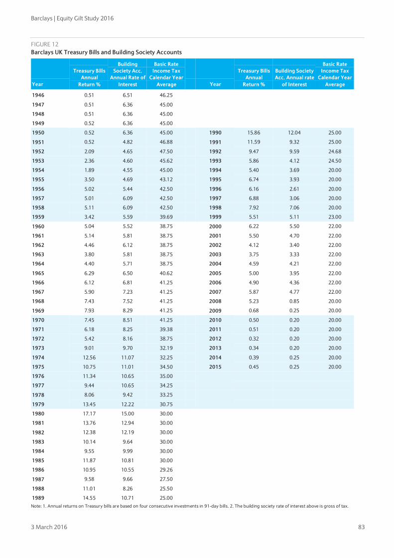
Barclays | Equity Gilt Study 2016
3 March 2016 83
FIGURE 12 Barclays UK Treasury Bills and Building Society Accounts
Year
Treasury Bills Annual
Return %
Building Society Acc.
Annual Rate of Interest
Basic Rate Income Tax
Calendar Year Average Year
Treasury Bills Annual
Return %
Building Society Acc. Annual rate
of Interest
Basic Rate Income Tax
Calendar Year Average
1946 0.51 6.51 46.25
1947 0.51 6.36 45.00
1948 0.51 6.36 45.00
1949 0.52 6.36 45.00
1950 0.52 6.36 45.00 1990 15.86 12.04 25.00
1951 0.52 4.82 46.88 1991 11.59 9.32 25.00
1952 2.09 4.65 47.50 1992 9.47 9.59 24.68
1953 2.36 4.60 45.62 1993 5.86 4.12 24.50
1954 1.89 4.55 45.00 1994 5.40 3.69 20.00
1955 3.50 4.69 43.12 1995 6.74 3.93 20.00
1956 5.02 5.44 42.50 1996 6.16 2.61 20.00
1957 5.01 6.09 42.50 1997 6.88 3.06 20.00
1958 5.11 6.09 42.50 1998 7.92 7.06 20.00
1959 3.42 5.59 39.69 1999 5.51 5.11 23.00
1960 5.04 5.52 38.75 2000 6.22 5.50 22.00
1961 5.14 5.81 38.75 2001 5.50 4.70 22.00
1962 4.46 6.12 38.75 2002 4.12 3.40 22.00
1963 3.80 5.81 38.75 2003 3.75 3.33 22.00
1964 4.40 5.71 38.75 2004 4.59 4.21 22.00
1965 6.29 6.50 40.62 2005 5.00 3.95 22.00
1966 6.12 6.81 41.25 2006 4.90 4.36 22.00
1967 5.90 7.23 41.25 2007 5.87 4.77 22.00
1968 7.43 7.52 41.25 2008 5.23 0.85 20.00
1969 7.93 8.29 41.25 2009 0.68 0.25 20.00
1970 7.45 8.51 41.25 2010 0.50 0.20 20.00
1971 6.18 8.25 39.38 2011 0.51 0.20 20.00
1972 5.42 8.16 38.75 2012 0.32 0.20 20.00
1973 9.01 9.70 32.19 2013 0.34 0.20 20.00
1974 12.56 11.07 32.25 2014 0.39 0.25 20.00
1975 10.75 11.01 34.50 2015 0.45 0.25 20.00
1976 11.34 10.65 35.00
1977 9.44 10.65 34.25
1978 8.06 9.42 33.25
1979 13.45 12.22 30.75
1980 17.17 15.00 30.00
1981 13.76 12.94 30.00
1982 12.38 12.19 30.00
1983 10.14 9.64 30.00
1984 9.55 9.99 30.00
1985 11.87 10.81 30.00
1986 10.95 10.55 29.26
1987 9.58 9.66 27.50
1988 11.01 8.26 25.50
1989 14.55 10.71 25.00 Note: 1. Annual returns on Treasury bills are based on four consecutive investments in 91-day bills. 2. The building society rate of interest above is gross of tax.
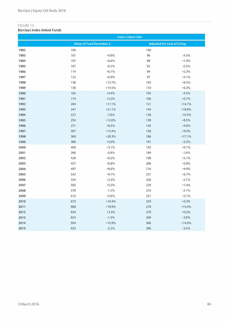
Barclays | Equity Gilt Study 2016
3 March 2016 84
FIGURE 13 Barclays Index-linked Funds
Index Linked Gilts
Value of Fund December £ Adjusted for Cost of Living
1982 100 100
1983 101 +0.8% 96 -4.3%
1984 107 +6.6% 98 +1.9%
1985 107 -0.2% 92 -5.5%
1986 114 +6.1% 94 +2.3%
1987 122 +6.9% 97 +3.1%
1988 138 +13.7% 103 +6.5%
1989 158 +14.5% 110 +6.3%
1990 165 +4.4% 105 -4.5%
1991 174 +5.2% 106 +0.7%
1992 204 +17.1% 121 +14.1%
1993 247 +21.1% 144 +18.9%
1994 227 -7.9% 128 -10.5%
1995 254 +12.0% 139 +8.5%
1996 271 +6.5% 145 +4.0%
1997 307 +13.4% 158 +9.4%
1998 369 +20.3% 186 +17.1%
1999 388 +5.0% 191 +3.2%
2000 400 +3.1% 192 +0.1%
2001 396 -0.9% 189 -1.6%
2002 428 +8.2% 198 +5.1%
2003 457 +6.8% 206 +3.9%
2004 497 +8.6% 216 +4.9%
2005 542 +9.1% 231 +6.7%
2006 554 +2.3% 226 -2.1%
2007 585 +5.5% 229 +1.4%
2008 578 -1.2% 224 -2.1%
2009 610 +5.6% 231 +3.1%
2010 673 +10.3% 243 +5.3%
2011 808 +19.9% 278 +14.4%
2012 834 +3.3% 279 +0.2%
2013 824 -1.3% 268 -3.9%
2014 954 +15.9% 306 +14.0%
2015 933 -2.2% 296 -3.4%

Barclays | Equity Gilt Study 2016
3 March 2016 85
FIGURE 14 Barclays US Equity Index
Year
Equity Price Index December
Equity Income Index December
Income Yield %
Equity Price Index Adjusted for Cost of
Living
Equity Income Index Adjusted for Cost of
Living
1925 100
100
1926 104 +4.3% 100
5.3 105 +5.5% 100
1927 132 +26.6% 119 +19.0% 5.0 137 +29.6% 122 +21.7%
1928 177 +33.7% 132 +11.3% 4.2 185 +35.3% 137 +12.7%
1929 144 -18.2% 98 -26.3% 3.8 150 -18.7% 101 -26.7%
1930 98 -32.1% 80 -17.7% 4.6 109 -27.5% 88 -12.1%
1931 51 -47.7% 54 -32.6% 5.9 63 -42.3% 66 -25.7%
1932 44 -14.1% 55 +1.7% 7.0 60 -4.2% 74 +13.3%
1933 66 +50.9% 53 -4.4% 4.4 90 +49.8% 71 -5.1%
1934 66 -1.0% 50 -5.7% 4.2 88 -2.4% 66 -7.1%
1935 92 +39.6% 71 +42.2% 4.3 119 +35.6% 91 +38.1%
1936 116 +26.7% 95 +34.1% 4.5 149 +24.9% 120 +32.2%
1937 72 -38.1% 69 -27.4% 5.3 90 -39.8% 85 -29.4%
1938 89 +23.0% 70 +1.6% 4.4 113 +26.5% 88 +4.5%
1939 86 -2.9% 75 +7.1% 4.8 110 -2.9% 95 +7.1%
1940 75 -12.8% 79 +5.7% 5.9 95 -13.4% 99 +5.0%
1941 63 -16.1% 81 +1.9% 7.1 73 -23.7% 92 -7.3%
1942 69 +9.1% 87 +8.3% 7.1 73 +0.0% 91 -0.7%
1943 84 +21.6% 80 -8.6% 5.3 86 +18.1% 81 -11.2%
1944 96 +15.5% 90 +12.7% 5.2 97 +12.9% 89 +10.2%
1945 129 +33.5% 98 +9.0% 4.2 127 +30.6% 95 +6.6%
1946 116 -10.2% 86 -12.6% 4.1 96 -24.0% 71 -26.0%
1947 113 -2.3% 115 +34.5% 5.7 87 -10.2% 87 +23.6%
1948 108 -4.1% 125 +8.1% 6.4 81 -6.9% 92 +5.0%
1949 122 +12.1% 156 +25.6% 7.2 92 +14.5% 117 +28.2%
1950 148 +21.7% 194 +24.3% 7.3 106 +14.9% 138 +17.3%
1951 169 +14.3% 178 -8.3% 5.9 114 +7.8% 119 -13.5%
1952 182 +7.4% 182 +2.2% 5.6 122 +6.6% 121 +1.4%
1953 173 -5.0% 175 -3.8% 5.7 115 -5.7% 115 -4.5%
1954 247 +43.4% 225 +28.5% 5.1 166 +44.4% 149 +29.4%
1955 298 +20.4% 228 +1.1% 4.3 199 +20.0% 150 +0.7%
1956 311 +4.4% 225 -1.4% 4.0 202 +1.3% 144 -4.2%
1957 267 -14.1% 205 -8.6% 4.3 168 -16.5% 128 -11.2%
1958 372 +39.3% 270 +31.6% 4.0 231 +36.9% 165 +29.3%
1959 406 +9.1% 240 -11.1% 3.3 247 +7.2% 145 -12.6%
1960 397 -2.2% 251 +4.5% 3.5 238 -3.5% 149 +3.1%
1961 490 +23.3% 266 +5.9% 3.0 292 +22.5% 157 +5.2%
1962 425 -13.3% 262 -1.3% 3.4 250 -14.4% 153 -2.6%
1963 497 +17.1% 291 +11.0% 3.3 288 +15.2% 167 +9.2%
1964 561 +12.8% 310 +6.6% 3.1 322 +11.8% 176 +5.5%
1965 623 +11.0% 343 +10.6% 3.1 350 +8.9% 191 +8.5%
1966 550 -11.7% 327 -4.7% 3.3 299 -14.6% 176 -7.9%
1967 686 +24.7% 381 +16.5% 3.1 362 +21.0% 199 +13.0%
1968 761 +10.9% 404 +6.1% 3.0 384 +5.9% 201 +1.3%
1969 658 -13.5% 361 -10.5% 3.1 312 -18.6% 170 -15.8%
1970 636 -3.4% 413 +14.4% 3.6 286 -8.5% 184 +8.4%

Barclays | Equity Gilt Study 2016
3 March 2016 86
Year
Equity Price Index December
Equity Income Index December
Income Yield %
Equity Price Index Adjusted for Cost of
Living
Equity Income Index Adjusted for Cost of
Living
1971 717 +12.8% 389 -5.9% 3.0 312 +9.2% 167 -8.9%
1972 819 +14.3% 405 +4.0% 2.8 345 +10.5% 168 +0.6%
1973 646 -21.2% 344 -15.0% 3.0 250 -27.5% 132 -21.8%
1974 445 -31.1% 348 +1.1% 4.4 154 -38.6% 119 -10.0%
1975 587 +31.8% 453 +30.3% 4.3 189 +23.3% 145 +21.9%
1976 715 +21.9% 515 +13.7% 4.0 220 +16.3% 157 +8.4%
1977 663 -7.3% 553 +7.3% 4.6 191 -13.1% 158 +0.5%
1978 685 +3.3% 629 +13.8% 5.1 181 -5.3% 164 +4.4%
1979 810 +18.3% 764 +21.4% 5.2 189 +4.4% 176 +7.2%
1980 1030 +27.1% 910 +19.2% 4.9 214 +13.0% 187 +5.9%
1981 944 -8.4% 804 -11.7% 4.7 180 -15.9% 151 -18.9%
1982 1078 +14.2% 1059 +31.7% 5.5 198 +10.0% 192 +26.9%
1983 1271 +17.9% 936 -11.6% 4.1 225 +13.6% 163 -14.9%
1984 1257 -1.1% 985 +5.3% 4.4 214 -4.9% 166 +1.3%
1985 1589 +26.5% 1141 +15.8% 4.0 260 +21.8% 185 +11.6%
1986 1777 +11.8% 1096 -3.9% 3.4 288 +10.6% 176 -5.0%
1987 1753 -1.4% 1012 -7.6% 3.2 272 -5.5% 155 -11.6%
1988 1980 +13.0% 1452 +43.5% 4.1 294 +8.2% 213 +37.4%
1989 2456 +24.0% 1594 +9.8% 3.6 349 +18.5% 224 +4.9%
1990 2225 -9.4% 1454 -8.8% 3.6 298 -14.6% 192 -14.0%
1991 2885 +29.6% 1640 +12.8% 3.2 374 +25.8% 210 +9.4%
1992 3061 +6.1% 1533 -6.5% 2.8 386 +3.1% 191 -9.2%
1993 3330 +8.8% 1547 +0.9% 2.6 409 +5.9% 188 -1.8%
1994 3221 -3.3% 1502 -2.9% 2.6 385 -5.8% 178 -5.4%
1995 4268 +32.5% 1876 +24.9% 2.4 498 +29.2% 216 +21.8%
1996 5069 +18.8% 1876 +0.0% 2.1 572 +15.0% 209 -3.2%
1997 6498 +28.2% 2011 +7.2% 1.7 721 +26.0% 221 +5.4%
1998 7831 +20.5% 2082 +3.5% 1.5 855 +18.6% 225 +1.9%
1999 9682 +23.6% 2308 +10.9% 1.3 1030 +20.4% 243 +8.0%
2000 8507 -12.1% 1688 -26.9% 1.1 875 -15.0% 172 -29.3%
2001 7448 -12.4% 1779 +5.4% 1.3 754 -13.8% 178 +3.8%
2002 5801 -22.1% 1660 -6.7% 1.6 574 -23.9% 162 -8.8%
2003 7587 +30.8% 2511 +51.2% 1.8 737 +28.4% 241 +48.5%
2004 8410 +10.8% 2970 +18.3% 2.0 791 +7.3% 276 +14.6%
2005 8862 +5.4% 2930 -1.4% 1.8 806 +1.9% 263 -4.6%
2006 10107 +14.0% 3474 +18.6% 1.9 896 +11.2% 305 +15.6%
2007 10638 +5.3% 3674 +5.7% 1.9 907 +1.1% 310 +1.6%
2008 6420 -39.65% 2639 -28.18% 2.3 547 -39.71% 222 -28.24%
2009 8223 +28.08% 3767 +42.76% 2.6 682 +24.69% 309 +38.98%
2010 9475 +15.23% 3691 -2.00% 2.2 774 +13.54% 298 -3.45%
2011 9181 -3.11% 3438 -6.88% 2.1 728 -5.89% 270 -9.56%
2012 10367 +12.92% 4719 +37.29% 2.5 808 +10.99% 364 +34.94%
2013 13237 +27.68% 5233 +10.89% 2.2 1017 +25.79% 397 +9.25%
2014
14327 +8.24% 5443 +4.01% 2.1 1092 +7.42% 410 +3.23%
2015
13785 -3.79% 5396 -0.86% 2.2 1044 -4.46% 404 -1.55%
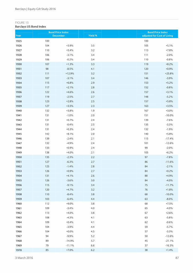
Barclays | Equity Gilt Study 2016
3 March 2016 87
FIGURE 15 Barclays US Bond Index
Year
Bond Price Index December
Yield %
Bond Price Index adjusted for Cost of Living
1925 100
100
1926 104
+3.9%
3.5
105
+5.1%
1927 110
+5.4%
3.2
113
+7.8%
1928 106
-3.1%
3.4
111
-2.0%
1929 106
-0.2%
3.4
110
-0.8%
1930 107
+1.3%
3.3
119
+8.2%
1931 98
-8.5%
4.1
120
+0.9%
1932 111
+12.9%
3.2
151
+25.8%
1933 107
-3.1%
3.4
146
-3.9%
1934 115
+6.8%
2.9
153
+5.2%
1935 117
+2.1%
2.8
152
-0.8%
1936 122
+4.6%
2.6
157
+3.1%
1937 119
-2.5%
2.7
148
-5.2%
1938 123
+2.8%
2.5
157
+5.8%
1939 127
+3.5%
2.3
163
+3.5%
1940 132
+3.8%
1.9
167
+3.0%
1941 131
-1.0%
2.0
151
-10.0%
1942 131
+0.7%
2.4
139
-7.6%
1943 131
-0.4%
2.5
135
-3.3%
1944 131
+0.3%
2.4
132
-1.9%
1945 142
+8.1%
2.0
140
+5.8%
1946 139
-2.4%
2.1
115
-17.4%
1947 132
-4.9%
2.4
101
-12.6%
1948 133
+0.9%
2.4
99
-2.0%
1949 138
+4.0%
2.1
105
+6.2%
1950 135
-2.3%
2.2
97
-7.8%
1951 127
-6.3%
2.7
86
-11.6%
1952 125
-1.4%
2.8
84
-2.1%
1953 126
+0.9%
2.7
84
+0.2%
1954 131
+4.1%
2.6
88
+4.9%
1955 126
-3.6%
3.0
84
-4.0%
1956 115
-9.1%
3.4
75
-11.7%
1957 120
+4.7%
3.2
76
+1.8%
1958 110
-8.4%
3.8
68
-10.0%
1959 103
-6.4%
4.4
63
-8.0%
1960 112
+9.0%
3.8
68
+7.5%
1961 109
-3.4%
4.0
65
-4.0%
1962 113
+4.0%
3.8
67
+2.6%
1963 108
-4.3%
4.1
63
-5.8%
1964 109 +0.4% 4.1 62 -0.6%
1965 104
-3.9%
4.4
59
-5.7%
1966 104
+0.0%
4.5
57
-3.3%
1967 94
-9.9%
5.2
50
-12.6%
1968 89
-14.9%
5.7
45
-21.1%
1969 79
-11.1%
6.6
37
-16.3%
1970 85
+7.0%
6.2
38
+1.4%

Barclays | Equity Gilt Study 2016
3 March 2016 88
Year
Bond Price Index December
Yield %
Bond Price Index adjusted for Cost of Living
1971 95
+12.2%
4.5
41
+8.6%
1972 96
+1.3%
4.5
40
-2.1%
1973 88
-8.8%
7.1
34
-16.1%
1974 84
-3.8%
7.7
29
-14.4%
1975 83
-1.7%
7.7
27
-8.0%
1976 91
+9.8%
6.9
28
+4.7%
1977 86
-6.0%
7.5
25
-11.9%
1978 77
-10.3%
8.8
20
-17.7%
1979 69
-10.0%
9.9
16
-20.5%
1980 60
-13.3%
11.6
12
-22.9%
1981 53
-11.5%
13.7
10
-18.7%
1982 65
+23.3%
10.5
12
+18.8%
1983 59
-9.4%
11.6
10
-12.7%
1984 61
+2.5%
11.3
10
-1.4%
1985 72
+18.7%
9.3
12
+14.3%
1986 84
+16.1%
7.6
14
+14.8%
1987 75
-11.0%
8.8
12
-14.8%
1988 74
-0.6%
8.8
11
-4.8%
1989 81
+9.5%
7.9
12
+4.6%
1990 79
-2.8%
8.2
11
-8.4%
1991 86
+9.1%
7.3
11
+5.9%
1992 86
-0.3%
7.3
11
-3.1%
1993 93
+8.8%
6.4
11
+5.9%
1994 80
-14.3%
7.9
10
-16.5%
1995 97
+21.1%
5.9
11
+18.1%
1996 90
-7.0%
6.6
10
-10.0%
1997 97
+7.7%
5.9
11
+5.9%
1998 103
+6.1%
5.3
11
+4.4%
1999 88
-14.5%
6.7
9
-16.8%
2000 100
+13.3%
5.5
10
+9.6%
2001 98
-2.1%
5.7
10
-3.6%
2002
108
+10.5%
4.8
11
+7.9%
2003
105
-2.9%
5.0
10
-4.7%
2004 107 +2.4% 4.8 10 -0.8%
2005 110 +2.2% 4.6 10 -1.2%
2006 105
-4.1%
4.8
9
-6.5%
2007 109
+4.1%
4.5
9
-0.0%
2008 131
+19.8%
3.1
11
+19.7%
2009 107
-17.9%
4.5
9
-20.1%
2010 113
+4.8%
4.1
9
+3.3%
2011 137
+21.7%
2.5
11
+18.2%
2012 138
+0.4%
2.7
11
-1.3%
2013 116
-15.4%
3.7
9
-16.7%
2014
140
+20.2%
2.4
11
+19.3%
2015
134
-4.0%
2.7
10
-4.7%
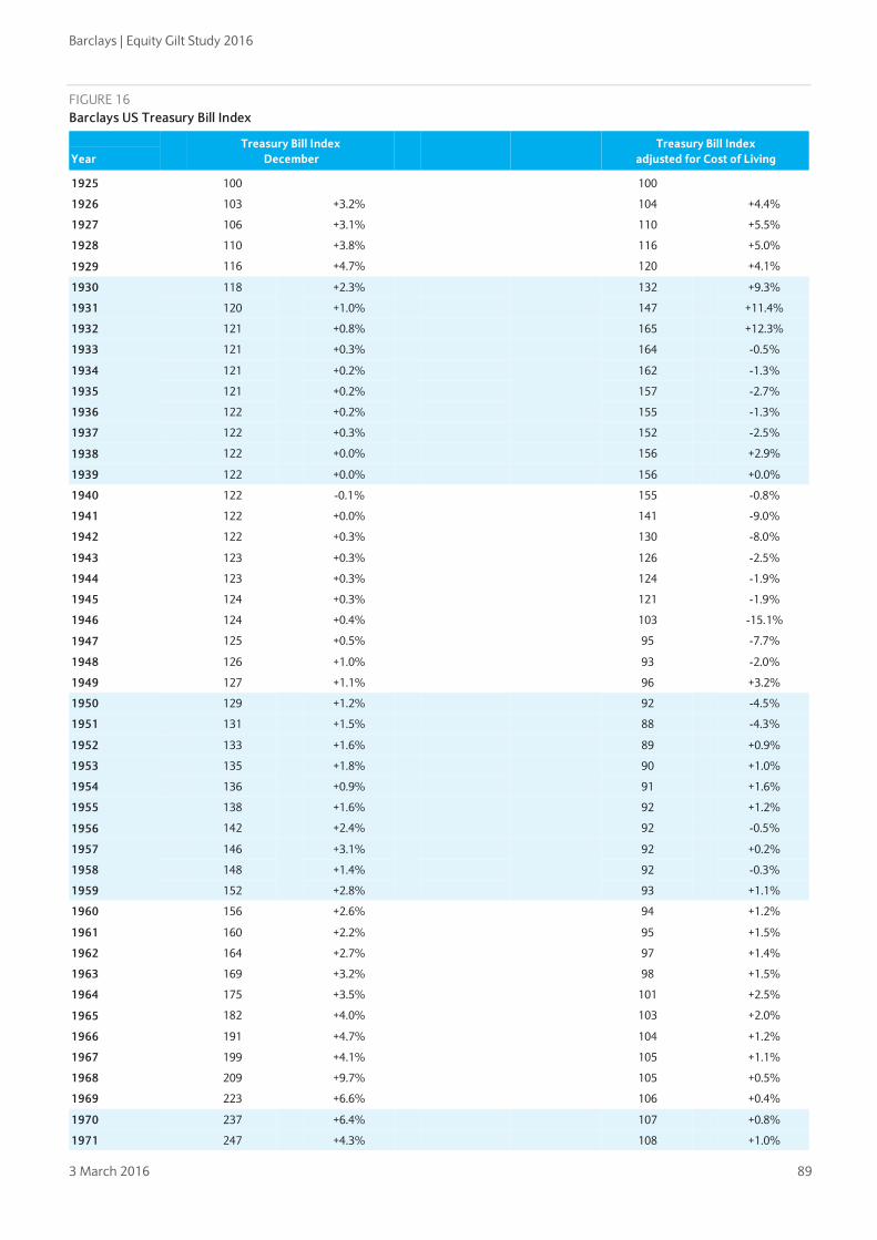
Barclays | Equity Gilt Study 2016
3 March 2016 89
FIGURE 16 Barclays US Treasury Bill Index
Year
Treasury Bill Index December
Treasury Bill Index adjusted for Cost of Living
1925 100
100
1926 103
+3.2%
104
+4.4%
1927 106
+3.1%
110
+5.5%
1928 110
+3.8%
116
+5.0%
1929 116
+4.7%
120
+4.1%
1930 118
+2.3%
132
+9.3%
1931 120
+1.0%
147
+11.4%
1932 121
+0.8%
165
+12.3%
1933 121
+0.3%
164
-0.5%
1934 121
+0.2%
162
-1.3%
1935 121
+0.2%
157
-2.7%
1936 122
+0.2%
155
-1.3%
1937 122
+0.3%
152
-2.5%
1938 122
+0.0%
156
+2.9%
1939 122
+0.0%
156
+0.0%
1940 122
-0.1%
155
-0.8%
1941 122
+0.0%
141
-9.0%
1942 122
+0.3%
130
-8.0%
1943 123
+0.3%
126
-2.5%
1944 123
+0.3%
124
-1.9%
1945 124
+0.3%
121
-1.9%
1946 124
+0.4%
103
-15.1%
1947 125
+0.5%
95
-7.7%
1948 126
+1.0%
93
-2.0%
1949 127
+1.1%
96
+3.2%
1950 129
+1.2%
92
-4.5%
1951 131
+1.5%
88
-4.3%
1952 133
+1.6%
89
+0.9%
1953 135
+1.8%
90
+1.0%
1954 136
+0.9%
91
+1.6%
1955 138
+1.6%
92
+1.2%
1956 142
+2.4%
92
-0.5%
1957 146
+3.1%
92
+0.2%
1958 148
+1.4%
92
-0.3%
1959 152
+2.8%
93
+1.1%
1960 156
+2.6%
94
+1.2%
1961 160
+2.2%
95
+1.5%
1962 164
+2.7%
97
+1.4%
1963 169
+3.2%
98
+1.5%
1964 175 +3.5% 101 +2.5%
1965 182
+4.0%
103
+2.0%
1966 191
+4.7%
104
+1.2%
1967 199
+4.1%
105
+1.1%
1968 209
+9.7%
105
+0.5%
1969 223
+6.6%
106
+0.4%
1970 237
+6.4%
107
+0.8%
1971 247
+4.3%
108
+1.0%
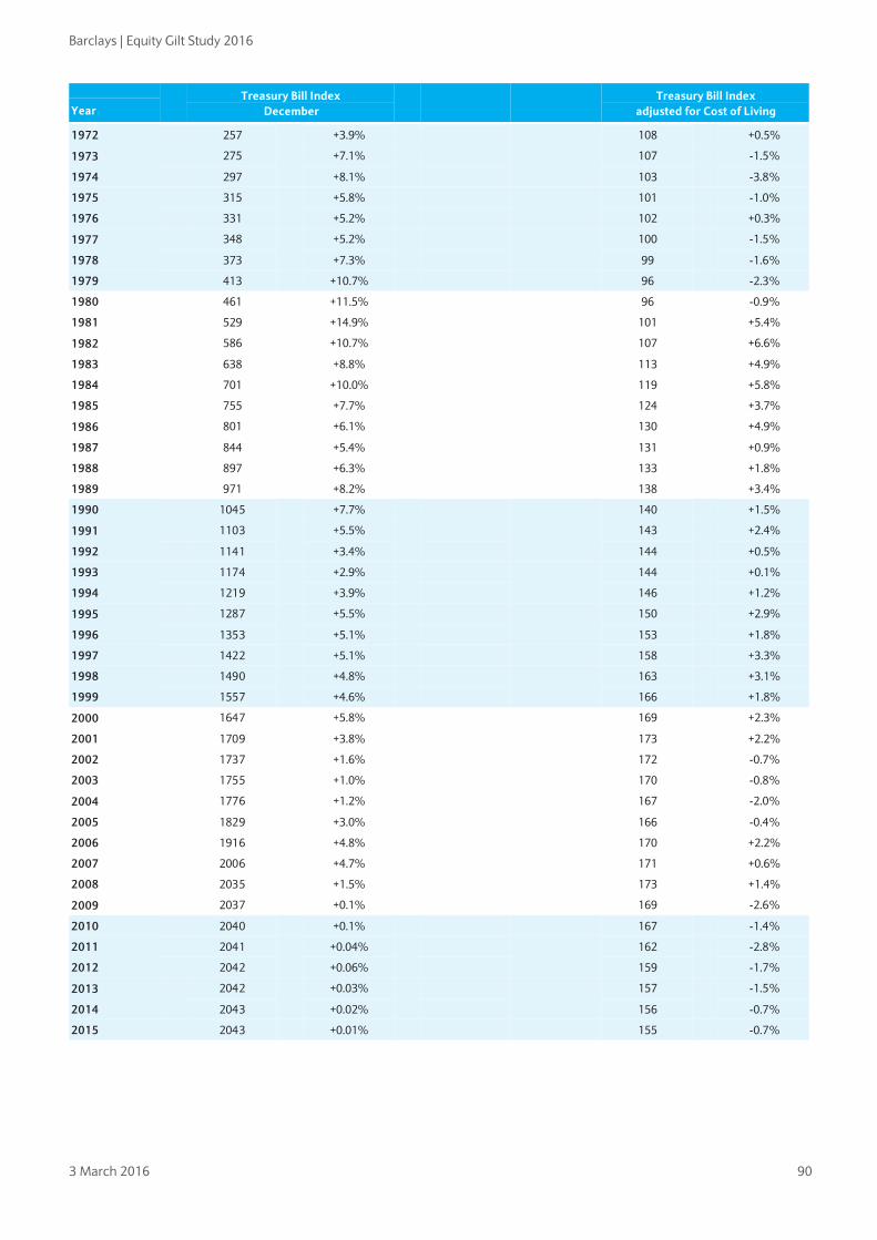
Barclays | Equity Gilt Study 2016
3 March 2016 90
Year
Treasury Bill Index December
Treasury Bill Index adjusted for Cost of Living
1972 257
+3.9%
108
+0.5%
1973 275
+7.1%
107
-1.5%
1974 297
+8.1%
103
-3.8%
1975 315
+5.8%
101
-1.0%
1976 331
+5.2%
102
+0.3%
1977 348
+5.2%
100
-1.5%
1978 373
+7.3%
99
-1.6%
1979 413
+10.7%
96
-2.3%
1980 461
+11.5%
96
-0.9%
1981 529
+14.9%
101
+5.4%
1982 586
+10.7%
107
+6.6%
1983 638
+8.8%
113
+4.9%
1984 701
+10.0%
119
+5.8%
1985 755
+7.7%
124
+3.7%
1986 801
+6.1%
130
+4.9%
1987 844
+5.4%
131
+0.9%
1988 897
+6.3%
133
+1.8%
1989 971
+8.2%
138
+3.4%
1990 1045
+7.7%
140
+1.5%
1991 1103
+5.5%
143
+2.4%
1992 1141
+3.4%
144
+0.5%
1993 1174
+2.9%
144
+0.1%
1994 1219
+3.9%
146
+1.2%
1995 1287
+5.5%
150
+2.9%
1996 1353
+5.1%
153
+1.8%
1997 1422
+5.1%
158
+3.3%
1998 1490
+4.8%
163
+3.1%
1999 1557
+4.6%
166
+1.8%
2000 1647
+5.8%
169
+2.3%
2001 1709
+3.8%
173
+2.2%
2002 1737
+1.6%
172
-0.7%
2003 1755
+1.0%
170
-0.8%
2004 1776
+1.2%
167
-2.0%
2005 1829
+3.0%
166
-0.4%
2006 1916
+4.8%
170
+2.2%
2007 2006
+4.7%
171
+0.6%
2008 2035
+1.5%
173
+1.4%
2009 2037
+0.1%
169
-2.6%
2010 2040
+0.1%
167
-1.4%
2011 2041
+0.04%
162
-2.8%
2012 2042
+0.06%
159
-1.7%
2013 2042
+0.03%
157
-1.5%
2014
2043
+0.02%
156
-0.7%
2015
2043
+0.01%
155
-0.7%

Barclays | Equity Gilt Study 2016
3 March 2016 91
CHAPTER 8
Total investment returns Our final chapter presents a series of tables showing the performance of equity and fixed-interest investments over any period of years since December 1899.
The first section reviews the performance of each asset class, taking inflation into account, since December 1960. On each page we provide two tables illustrating the same information in alternative forms. The first table shows the average annual real rate of return; the second shows the real value of a portfolio at the end of each year, which includes reinvested income. This section provides data on equities and gilts, with dividend income reinvested gross. Finally, we provide figures for Treasury bills and building society shares.
The final pullout section provides the annual real rate of return on UK and US equities and bonds (with reinvestment of income for each year since 1899 for the UK, and since 1925 for the US). There is also a table showing the real capital value of equities for the UK. The sources for all data in this chapter are the Barclays indices, as outlined in Chapter 7.
• Equities – income gross
• Gilts – income gross
• Treasury Bills – income gross
• Building Society Shares – income gross
• Index-linked gilts
• UK and US real bond returns – income gross
• UK and US real equities returns – income gross
• UK Equities – real capital value
Sreekala Kochugovindan +44 (0)20 7773 2234 sreekala.kochugovindan@ barclays.com Barclays, UK
1960-2015
UK: 1899-2015 US: 1925-2015
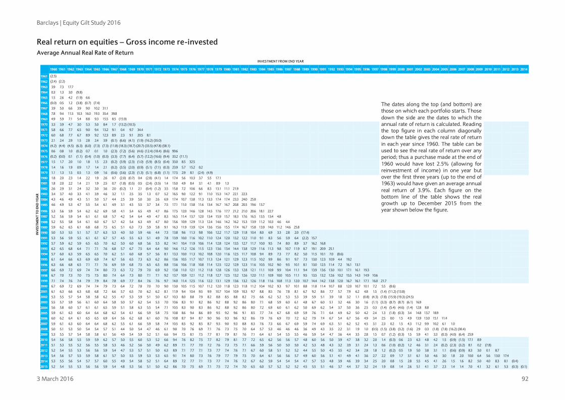
Barclays | Equity Gilt Study 2016
3 March 2016 92
Real return on equities – Gross income re-invested Average Annual Real Rate of Return
INVESTMENT FROM END YEAR
INV
ESTM
ENT
TO E
ND
YEA
R
1960 1961 1962 1963 1964 1965 1966 1967 1968 1969 1970 1971 1972 1973 1974 1975 1976 1977 1978 1979 1980 1981 1982 1983 1984 1985 1986 1987 1988 1989 1990 1991 1992 1993 1994 1995 1996 1997 1998 1999 2000 2001 2002 2003 2004 2005 2006 2007 2008 2009 2010 2011 2012 2013 2014
1961 (2.5)
1962 (2.4) (2.2)
1963 3.9 7.3 17.7
1964 0.3 1.3 3.0 (9.8)
1965 1.5 2.6 4.2 (1.9) 6.6
1966 (0.0) 0.5 1.2 (3.8) (0.7) (7.4)
The dates along the top (and bottom) are those on which each portfolio starts. Those down the side are the dates to which the annual rate of return is calculated. Reading the top figure in each column diagonally down the table gives the real rate of return in each year since 1960. The table can be used to see the real rate of return over any period; thus a purchase made at the end of 1960 would have lost 2.5% (allowing for reinvestment of income) in one year but over the first three years (up to the end of 1963) would have given an average annual real return of 3.9%. Each figure on the bottom line of the table shows the real growth up to December 2015 from the year shown below the figure.
1967 3.9 5.0 6.6 3.9 9.0 10.2 31.1
1968 7.8 9.4 11.5 10.3 16.0 19.3 35.4 39.8
1969 4.9 5.9 7.1 5.4 8.8 9.3 15.5 8.5 (15.9)
1970 3.3 3.9 4.7 3.0 5.3 5.0 8.4 1.7 (13.2) (10.5)
1971 5.8 6.6 7.7 6.5 9.0 9.4 13.2 9.1 0.4 9.7 34.4
1972 6.0 6.8 7.7 6.7 8.9 9.2 12.3 8.9 2.3 9.1 20.5 8.1
1973 2.1 2.4 2.9 1.5 2.8 2.4 3.9 (0.1) (6.6) (4.1) (1.9) (16.2) (35.0)
1974 (4.2) (4.4) (4.5) (6.3) (6.0) (7.3) (7.3) (11.8) (18.3) (18.7) (20.7) (33.5) (47.8) (58.1)
1975 0.6 0.8 1.0 (0.2) 0.7 0.1 1.0 (2.3) (7.2) (5.6) (4.6) (12.4) (18.4) (8.6) 99.6
1976 (0.2) (0.0) 0.1 (1.1) (0.4) (1.0) (0.3) (3.3) (7.7) (6.4) (5.7) (12.2) (16.6) (9.4) 33.2 (11.1)
1977 1.5 1.7 2.0 1.0 1.8 1.5 2.3 (0.2) (3.9) (2.3) (1.0) (5.9) (8.5) (0.4) 33.0 8.5 32.5
1978 1.4 1.6 1.9 0.9 1.7 1.4 2.1 (0.2) (3.5) (2.0) (0.9) (5.1) (7.1) (0.3) 23.9 5.7 15.2 0.2
1979 1.1 1.3 1.5 0.5 1.3 0.9 1.6 (0.6) (3.6) (2.3) (1.3) (5.1) (6.8) (1.1) 17.5 2.9 8.1 (2.4) (4.9)
1980 1.8 2.0 2.3 1.4 2.2 1.9 2.6 0.7 (2.0) (0.7) 0.4 (2.8) (4.1) 1.4 17.4 5.6 10.3 3.7 5.5 17.1
1981 1.8 2.0 2.2 1.4 2.1 1.9 2.5 0.7 (1.8) (0.5) 0.5 (2.4) (3.5) 1.4 15.0 4.9 8.4 3.1 4.1 8.9 1.3
1982 2.6 2.9 3.1 2.4 3.2 3.0 3.6 2.0 (0.2) 1.1 2.1 (0.4) (1.2) 3.5 15.8 7.2 10.6 6.6 8.3 13.1 11.1 21.9
1983 3.4 3.7 4.0 3.3 4.1 3.9 4.6 3.2 1.1 2.5 3.5 1.3 0.7 5.2 16.5 9.0 12.2 9.1 11.0 15.3 14.7 22.1 22.3
1984 4.3 4.6 4.9 4.3 5.1 5.0 5.7 4.4 2.5 3.9 5.0 3.0 2.6 6.9 17.4 10.7 13.8 11.3 13.3 17.4 17.4 23.3 24.0 25.8
1985 4.6 4.9 5.3 4.7 5.5 5.4 6.1 4.9 3.1 4.5 5.5 3.7 3.4 7.5 17.1 11.0 13.8 11.6 13.4 16.7 16.7 20.8 20.5 19.6 13.7
1986 5.3 5.6 5.9 5.4 6.2 6.2 6.9 5.8 4.1 5.4 6.5 4.9 4.7 8.6 17.5 12.0 14.6 12.8 14.5 17.6 17.7 21.2 21.0 20.6 18.1 22.7
1987 5.2 5.6 5.9 5.4 6.1 6.1 6.8 5.7 4.2 5.4 6.4 4.9 4.7 8.3 16.5 11.4 13.7 12.0 13.4 15.9 15.7 18.3 17.6 16.5 13.5 13.4 4.8
1988 5.2 5.5 5.8 5.4 6.1 6.0 6.7 5.7 4.2 5.4 6.3 4.9 4.7 8.0 15.6 10.9 12.9 11.3 12.4 14.6 14.2 16.2 15.3 13.9 11.2 10.3 4.6 4.4
1989 5.9 6.2 6.5 6.1 6.8 6.8 7.5 6.5 5.1 6.3 7.3 5.9 5.8 9.1 16.3 11.9 13.9 12.4 13.6 15.6 15.5 17.4 16.7 15.8 13.9 14.0 11.2 14.6 25.8
1990 5.0 5.3 5.5 5.1 5.7 5.7 6.3 5.3 4.0 5.0 5.9 4.6 4.4 7.3 13.8 9.6 11.3 9.8 10.6 12.2 11.7 12.9 11.8 10.4 8.0 6.9 3.3 2.8 2.0 (17.4)
1991 5.3 5.6 5.9 5.5 6.1 6.1 6.7 5.7 4.5 5.5 6.3 5.1 4.9 7.8 13.9 10.0 11.6 10.2 11.0 12.4 12.0 13.2 12.2 11.0 9.1 8.3 5.6 5.9 6.4 (2.2) 15.7
1992 5.7 5.9 6.2 5.9 6.5 6.5 7.0 6.2 5.0 6.0 6.8 5.6 5.5 8.2 14.1 10.4 11.9 10.6 11.4 12.8 12.4 13.5 12.7 11.7 10.0 9.5 7.4 8.0 8.9 3.7 16.2 16.8
1993 6.2 6.5 6.8 6.4 7.1 7.1 7.6 6.8 5.7 6.7 7.5 6.4 6.4 9.0 14.6 11.2 12.6 11.5 12.3 13.6 13.4 14.4 13.8 12.9 11.6 11.3 9.8 10.7 11.9 8.7 19.1 20.9 25.1
1994 5.7 6.0 6.3 5.9 6.5 6.5 7.0 6.2 5.1 6.0 6.8 5.7 5.6 8.1 13.3 10.0 11.3 10.2 10.8 12.0 11.6 12.5 11.7 10.8 9.4 8.9 7.3 7.7 8.2 5.0 11.5 10.1 7.0 (8.6)
1995 6.1 6.4 6.6 6.3 6.9 6.9 7.4 6.7 5.6 6.5 7.3 6.3 6.2 8.6 13.6 10.5 11.7 10.7 11.3 12.4 12.1 12.9 12.3 11.5 10.2 9.9 8.6 9.1 9.7 7.3 13.0 12.3 10.9 4.4 19.2
1996 6.3 6.6 6.8 6.5 7.1 7.1 7.6 6.9 5.9 6.8 7.5 6.5 6.5 8.8 13.6 10.6 11.8 10.8 11.4 12.5 12.2 12.9 12.3 11.6 10.5 10.2 9.0 9.5 10.1 8.1 13.0 12.5 11.4 7.2 16.1 13.1
1997 6.6 6.9 7.2 6.9 7.4 7.4 8.0 7.3 6.3 7.2 7.9 7.0 6.9 9.2 13.8 11.0 12.1 11.2 11.8 12.8 12.6 13.3 12.8 12.1 11.1 10.9 9.9 10.4 11.1 9.4 13.9 13.6 13.0 10.1 17.1 16.1 19.3
1998 6.7 7.0 7.3 7.0 7.5 7.5 8.0 7.4 6.4 7.3 8.0 7.1 7.1 9.2 13.7 10.9 12.1 11.2 11.8 12.7 12.5 13.2 12.6 12.0 11.1 10.9 10.0 10.5 11.1 9.5 13.5 13.2 12.6 10.2 15.5 14.3 14.9 10.6
1999 7.1 7.4 7.6 7.4 7.9 7.9 8.4 7.8 6.9 7.7 8.4 7.6 7.6 9.7 14.0 11.4 12.5 11.6 12.2 13.1 12.9 13.6 13.2 12.6 11.8 11.6 10.8 11.3 12.0 10.7 14.4 14.2 13.8 12.0 16.7 16.1 17.1 16.0 21.7
2000 6.7 6.9 7.2 6.9 7.4 7.4 7.9 7.3 6.4 7.2 7.8 7.0 7.0 9.0 13.0 10.5 11.5 10.7 11.2 12.0 11.8 12.3 11.8 11.2 10.4 10.2 9.3 9.7 10.1 8.8 11.8 11.4 10.7 8.8 12.0 10.7 10.1 7.2 5.5 (8.6)
2001 6.1 6.3 6.6 6.3 6.8 6.8 7.2 6.6 5.7 6.5 7.0 6.2 6.2 8.1 11.9 9.4 10.4 9.5 9.9 10.7 10.4 10.9 10.3 9.7 8.8 8.5 7.6 7.8 8.1 6.7 9.2 8.6 7.7 5.7 7.9 6.2 4.8 1.5 (1.4) (11.2) (13.8)
2002 5.3 5.5 5.7 5.4 5.8 5.8 6.2 5.5 4.7 5.3 5.9 5.1 5.0 6.7 10.3 8.0 8.8 7.9 8.2 8.8 8.5 8.8 8.2 7.5 6.6 6.2 5.2 5.3 5.3 3.9 5.9 5.1 3.9 1.8 3.2 1.1 (0.8) (4.3) (7.8) (15.9) (19.3) (24.5)
2003 5.5 5.7 5.9 5.6 6.1 6.0 6.4 5.8 5.0 5.7 6.2 5.4 5.3 7.0 10.6 8.3 9.1 8.2 8.6 9.2 8.8 9.2 8.6 8.0 7.1 6.8 5.9 6.0 6.1 4.8 6.7 6.0 5.1 3.2 4.6 3.0 1.6 (1.1) (3.3) (8.7) (8.7) (6.1) 16.9
2004 5.6 5.8 6.0 5.7 6.1 6.1 6.5 5.9 5.1 5.8 6.3 5.5 5.4 7.1 10.5 8.3 9.0 8.3 8.6 9.2 8.8 9.2 8.6 8.0 7.2 6.9 6.0 6.1 6.2 5.0 6.9 6.2 5.4 3.7 5.0 3.6 2.5 0.3 (1.4) (5.4) (4.6) (1.4) 12.8 8.8
2005 5.9 6.1 6.3 6.0 6.4 6.4 6.8 6.2 5.4 6.1 6.6 5.9 5.8 7.5 10.8 8.6 9.4 8.6 8.9 9.5 9.2 9.6 9.1 8.5 7.7 7.4 6.7 6.8 6.9 5.9 7.6 7.1 6.4 4.9 6.2 5.0 4.2 2.4 1.3 (1.8) (0.3) 3.4 14.8 13.7 18.9
2006 6.0 6.2 6.4 6.1 6.5 6.5 6.9 6.4 5.6 6.2 6.8 6.1 6.0 7.6 10.8 8.7 9.4 8.7 9.0 9.6 9.3 9.6 9.2 8.6 7.9 7.6 6.9 7.0 7.2 6.2 7.9 7.4 6.7 5.4 6.7 5.6 4.9 3.4 2.5 0.0 1.5 4.9 13.9 13.0 15.1 11.4
2007 5.9 6.1 6.3 6.0 6.4 6.4 6.8 6.2 5.5 6.1 6.6 5.9 5.8 7.4 10.5 8.5 9.2 8.5 8.7 9.3 9.0 9.3 8.8 8.3 7.6 7.3 6.6 6.7 6.9 5.9 7.4 6.9 6.3 5.1 6.2 5.2 4.5 3.1 2.3 0.2 1.5 4.3 11.2 9.9 10.2 6.1 1.0
2008 5.0 5.1 5.3 5.0 5.4 5.4 5.7 5.1 4.4 5.0 5.4 4.7 4.6 6.1 9.0 7.0 7.6 6.9 7.1 7.6 7.3 7.5 7.0 6.4 5.7 5.3 4.6 4.6 4.6 3.6 4.9 4.3 3.5 2.2 3.1 1.9 1.0 (0.5) (1.5) (3.8) (3.2) (1.6) 2.9 0.3 (1.8) (7.8) (16.2) (30.4)
2009 5.3 5.5 5.7 5.4 5.8 5.8 6.1 5.6 4.9 5.4 5.9 5.2 5.1 6.6 9.4 7.5 8.1 7.5 7.7 8.1 7.9 8.1 7.6 7.1 6.4 6.1 5.4 5.5 5.5 4.6 5.9 5.4 4.7 3.6 4.4 3.5 2.8 1.5 0.7 (1.2) (0.3) 1.5 5.9 4.1 3.3 (0.3) (4.0) (6.4) 25.9
2010 5.4 5.6 5.8 5.5 5.9 5.9 6.2 5.7 5.0 5.5 6.0 5.3 5.2 6.6 9.4 7.6 8.2 7.5 7.7 8.2 7.9 8.1 7.7 7.2 6.5 6.2 5.6 5.6 5.7 4.8 6.0 5.6 5.0 3.9 4.7 3.8 3.2 2.0 1.4 (0.3) 0.6 2.3 6.3 4.8 4.2 1.5 (0.9) (1.5) 17.1 8.9
2011 5.1 5.3 5.5 5.2 5.6 5.5 5.8 5.3 4.6 5.2 5.6 5.0 4.9 6.2 8.9 7.1 7.7 7.0 7.2 7.6 7.3 7.5 7.1 6.6 5.9 5.6 5.0 5.0 5.0 4.2 5.3 4.8 4.3 3.2 3.9 3.1 2.4 1.3 0.6 (1.0) (0.2) 1.2 4.6 3.1 2.4 (0.2) (2.3) (3.2) 8.1 0.2 (7.8)
2012 5.2 5.4 5.5 5.3 5.6 5.6 5.9 5.4 4.7 5.3 5.7 5.1 5.0 6.3 8.9 7.1 7.7 7.1 7.3 7.7 7.4 7.6 7.1 6.7 6.0 5.8 5.1 5.2 5.2 4.4 5.5 5.0 4.5 3.5 4.2 3.4 2.8 1.8 1.2 (0.2) 0.5 1.9 5.0 3.8 3.1 1.1 (0.6) (0.9) 8.3 3.0 0.1 8.7
2013 5.4 5.6 5.7 5.5 5.9 5.8 6.1 5.7 5.0 5.5 5.9 5.3 5.3 6.5 9.1 7.4 8.0 7.3 7.6 7.9 7.7 7.9 7.5 7.0 6.4 6.1 5.6 5.6 5.7 4.9 6.0 5.6 5.1 4.1 4.9 4.1 3.6 2.7 2.2 0.9 1.7 3.1 6.1 5.0 4.6 3.0 1.8 2.0 10.0 6.4 5.6 13.0 17.4
2014 5.3 5.5 5.6 5.4 5.7 5.7 6.0 5.5 4.9 5.4 5.8 5.2 5.1 6.4 8.9 7.2 7.7 7.1 7.3 7.7 7.4 7.6 7.2 6.7 6.2 5.9 5.4 5.4 5.4 4.7 5.7 5.3 4.8 3.9 4.6 3.9 3.4 2.5 2.0 0.8 1.5 2.8 5.5 4.5 4.1 2.6 1.5 1.6 8.2 5.0 4.0 8.3 8.1 (0.4)
2015 5.2 5.4 5.5 5.3 5.6 5.6 5.9 5.4 4.8 5.3 5.6 5.1 5.0 6.2 8.6 7.0 7.5 6.9 7.1 7.5 7.2 7.4 7.0 6.5 6.0 5.7 5.2 5.2 5.2 4.5 5.5 5.1 4.6 3.7 4.4 3.7 3.2 2.4 1.9 0.8 1.4 2.6 5.1 4.1 3.7 2.3 1.4 1.4 7.0 4.1 3.2 6.1 5.3 (0.3) (0.1)
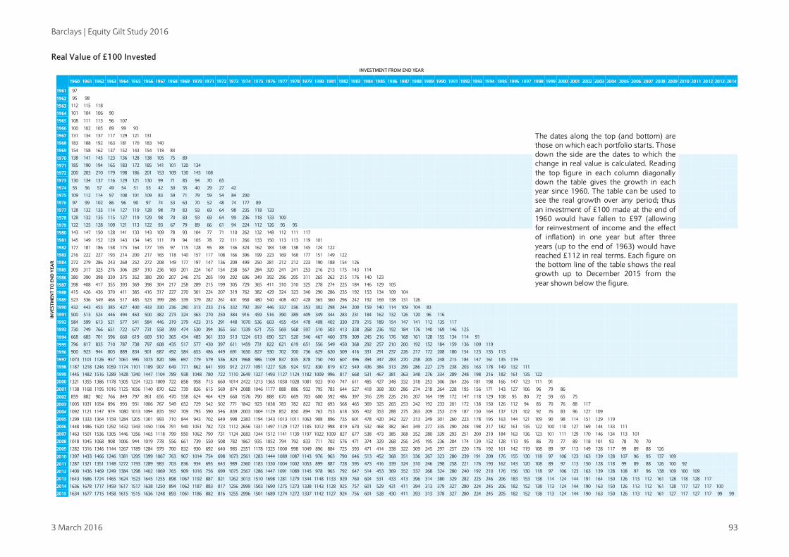
Barclays | Equity Gilt Study 2016
3 March 2016 93
Real Value of £100 Invested INVESTMENT FROM END YEAR
INV
ESTM
ENT
TO E
ND
YEA
R
1960 1961 1962 1963 1964 1965 1966 1967 1968 1969 1970 1971 1972 1973 1974 1975 1976 1977 1978 1979 1980 1981 1982 1983 1984 1985 1986 1987 1988 1989 1990 1991 1992 1993 1994 1995 1996 1997 1998 1999 2000 2001 2002 2003 2004 2005 2006 2007 2008 2009 2010 2011 2012 2013 2014
1961 97
1962 95 98
1963 112 115 118
1964 101 104 106 90
1965 108 111 113 96 107
1966 100 102 105 89 99 93 The dates along the top (and bottom) are
those on which each portfolio starts. Those down the side are the dates to which the change in real value is calculated. Reading the top figure in each column diagonally down the table gives the growth in each year since 1960. The table can be used to see the real growth over any period; thus an investment of £100 made at the end of 1960 would have fallen to £97 (allowing for reinvestment of income and the effect of inflation) in one year but after three years (up to the end of 1963) would have reached £112 in real terms. Each figure on the bottom line of the table shows the real growth up to December 2015 from the year shown below the figure.
1967 131 134 137 117 129 121 131
1968 183 188 192 163 181 170 183 140
1969 154 158 162 137 152 143 154 118 84
1970 138 141 145 123 136 128 138 105 75 89
1971 185 190 194 165 183 172 185 141 101 120 134
1972 200 205 210 179 198 186 201 153 109 130 145 108
1973 130 134 137 116 129 121 130 99 71 85 94 70 65
1974 55 56 57 49 54 51 55 42 30 35 40 29 27 42
1975 109 112 114 97 108 101 109 83 59 71 79 59 54 84 200
1976 97 99 102 86 96 90 97 74 53 63 70 52 48 74 177 89
1977 128 132 135 114 127 119 128 98 70 83 93 69 64 98 235 118 133
1978 128 132 135 115 127 119 129 98 70 83 93 69 64 99 236 118 133 100
1979 122 125 128 109 121 113 122 93 67 79 89 66 61 94 224 112 126 95 95
1980 143 147 150 128 141 133 143 109 78 93 104 77 71 110 262 132 148 112 111 117
1981 145 149 152 129 143 134 145 111 79 94 105 78 72 111 266 133 150 113 113 119 101
1982 177 181 186 158 175 164 177 135 97 115 128 95 88 136 324 162 183 138 138 145 124 122
1983 216 222 227 193 214 200 217 165 118 140 157 117 108 166 396 199 223 169 168 177 151 149 122
1984 272 279 286 243 269 252 272 208 149 177 197 147 136 209 499 250 281 212 212 223 190 188 154 126
1985 309 317 325 276 306 287 310 236 169 201 224 167 154 238 567 284 320 241 241 253 216 213 175 143 114
1986 380 390 398 339 375 352 380 290 207 246 275 205 190 292 696 349 392 296 295 311 265 262 215 176 140 123
1987 398 408 417 355 393 369 398 304 217 258 289 215 199 305 729 365 411 310 310 325 278 274 225 184 146 129 105
1988 415 426 436 370 411 385 416 317 227 270 301 224 207 319 762 382 429 324 323 340 290 286 235 192 153 134 109 104
1989 523 536 549 466 517 485 523 399 286 339 379 282 261 401 958 480 540 408 407 428 365 360 296 242 192 169 138 131 126
1990 432 443 453 385 427 400 433 330 236 280 313 233 216 332 792 397 446 337 336 353 302 298 244 200 159 140 114 109 104 83
1991 500 513 524 446 494 463 500 382 273 324 363 270 250 384 916 459 516 390 389 409 349 344 283 231 184 162 132 126 120 96 116
1992 584 599 613 521 577 541 584 446 319 379 423 315 291 448 1070 536 603 455 454 478 408 402 330 270 215 189 154 147 141 112 135 117
1993 730 749 766 651 722 677 731 558 399 474 530 394 365 561 1339 671 755 569 568 597 510 503 413 338 268 236 192 184 176 140 169 146 125
1994 668 685 701 596 660 619 669 510 365 434 485 361 333 513 1224 613 690 521 520 546 467 460 378 309 245 216 176 168 161 128 155 134 114 91
1995 796 817 835 710 787 738 797 608 435 517 577 430 397 611 1459 731 822 621 619 651 556 549 450 368 292 257 210 200 192 152 184 159 136 109 119
1996 900 923 944 803 889 834 901 687 492 584 653 486 449 691 1650 827 930 702 700 736 629 620 509 416 331 291 237 226 217 172 208 180 154 123 135 113
1997 1073 1101 1126 957 1061 995 1075 820 586 697 779 579 536 824 1968 986 1109 837 835 878 750 740 607 496 394 347 283 270 258 205 248 215 184 147 161 135 119
1998 1187 1218 1246 1059 1174 1101 1189 907 649 771 862 641 593 912 2177 1091 1227 926 924 972 830 819 672 549 436 384 313 299 286 227 275 238 203 163 178 149 132 111
1999 1445 1482 1516 1289 1428 1340 1447 1104 789 938 1048 780 722 1110 2649 1327 1493 1127 1124 1182 1009 996 817 668 531 467 381 363 348 276 334 289 248 198 216 182 161 135 122
2000 1321 1355 1386 1178 1305 1224 1323 1009 722 858 958 713 660 1014 2422 1213 1365 1030 1028 1081 923 910 747 611 485 427 348 332 318 253 306 264 226 181 198 166 147 123 111 91
2001 1138 1168 1195 1016 1125 1056 1140 870 622 739 826 615 569 874 2088 1046 1177 888 886 932 795 785 644 527 418 368 300 286 274 218 264 228 195 156 171 143 127 106 96 79 86
2002 859 882 902 766 849 797 861 656 470 558 624 464 429 660 1576 790 888 670 669 703 600 592 486 397 316 278 226 216 207 164 199 172 147 118 129 108 95 80 72 59 65 75
2003 1005 1031 1054 896 993 931 1006 767 549 652 729 542 502 771 1842 923 1038 783 782 822 702 693 568 465 369 325 265 253 242 192 233 201 172 138 150 126 112 94 85 70 76 88 117
2004 1092 1121 1147 974 1080 1013 1094 835 597 709 793 590 546 839 2003 1004 1129 852 850 894 763 753 618 505 402 353 288 275 263 209 253 219 187 150 164 137 121 102 92 76 83 96 127 109
2005 1299 1333 1364 1159 1284 1205 1301 993 710 844 943 702 649 998 2383 1194 1343 1013 1011 1063 908 896 735 601 478 420 342 327 313 249 301 260 223 178 195 163 144 121 109 90 98 114 151 129 119
2006 1448 1486 1520 1292 1432 1343 1450 1106 791 940 1051 782 723 1112 2656 1331 1497 1129 1127 1185 1012 998 819 670 532 468 382 364 349 277 335 290 248 198 217 182 161 135 122 100 110 127 169 144 133 111
2007 1463 1501 1536 1305 1446 1356 1465 1118 799 950 1062 790 731 1124 2683 1344 1512 1141 1139 1197 1022 1009 827 677 538 473 385 368 352 280 339 293 251 200 219 184 163 136 123 101 111 129 170 146 134 113 101
2008 1018 1045 1068 908 1006 944 1019 778 556 661 739 550 508 782 1867 935 1052 794 792 833 711 702 576 471 374 329 268 256 245 195 236 204 174 139 152 128 113 95 86 70 77 89 118 101 93 78 70 70
2009 1282 1316 1346 1144 1267 1189 1284 979 700 832 930 692 640 985 2351 1178 1325 1000 998 1049 896 884 725 593 471 414 338 322 309 245 297 257 220 176 192 161 142 119 108 89 97 113 149 128 117 99 89 88 126
2010 1397 1433 1466 1246 1381 1295 1399 1067 763 907 1014 754 698 1073 2561 1283 1444 1089 1087 1143 976 963 790 646 513 452 368 351 336 267 323 280 239 191 209 176 155 130 118 97 106 123 163 139 128 107 96 95 137 109
2011 1287 1321 1351 1148 1272 1193 1289 983 703 836 934 695 643 989 2360 1183 1330 1004 1002 1053 899 887 728 595 473 416 339 324 310 246 298 258 221 176 193 162 143 120 108 89 97 113 150 128 118 99 89 88 126 100 92
2012 1400 1436 1469 1249 1384 1298 1402 1069 765 909 1016 756 699 1075 2567 1286 1447 1091 1089 1145 978 965 792 647 514 453 369 352 337 268 324 280 240 192 210 176 156 130 118 97 106 123 163 139 128 108 97 96 138 109 100 109
2013 1643 1686 1724 1465 1624 1523 1645 1255 898 1067 1192 887 821 1262 3013 1510 1698 1281 1279 1344 1148 1133 929 760 604 531 433 413 396 314 380 329 282 225 246 206 183 153 138 114 124 144 191 164 150 126 113 112 161 128 118 128 117
2014 1636 1678 1717 1459 1617 1517 1638 1250 894 1062 1187 883 817 1256 2999 1503 1690 1275 1273 1338 1143 1128 925 757 601 529 431 411 394 313 379 327 280 224 245 206 182 152 138 113 124 144 190 163 150 126 113 112 161 128 117 127 117 100
2015 1634 1677 1715 1458 1615 1515 1636 1248 893 1061 1186 882 816 1255 2996 1501 1689 1274 1272 1337 1142 1127 924 756 601 528 430 411 393 313 378 327 280 224 245 205 182 152 138 113 124 144 190 163 150 126 113 112 161 127 117 127 117 99 99
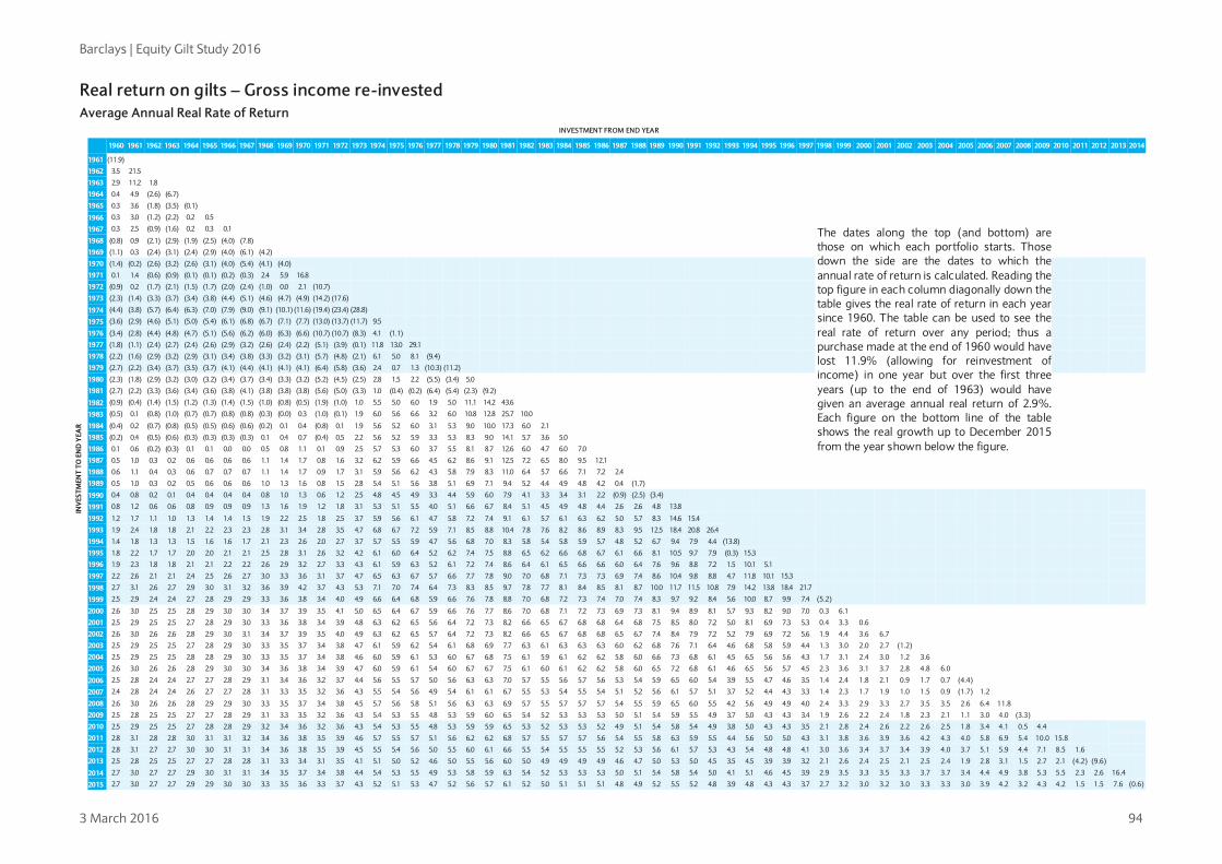
Barclays | Equity Gilt Study 2016
3 March 2016 94
Real return on gilts – Gross income re-invested Average Annual Real Rate of Return
INVESTMENT FROM END YEAR
INV
ESTM
ENT
TO E
ND
YEA
R
1960 1961 1962 1963 1964 1965 1966 1967 1968 1969 1970 1971 1972 1973 1974 1975 1976 1977 1978 1979 1980 1981 1982 1983 1984 1985 1986 1987 1988 1989 1990 1991 1992 1993 1994 1995 1996 1997 1998 1999 2000 2001 2002 2003 2004 2005 2006 2007 2008 2009 2010 2011 2012 2013 2014
1961 (11.9)
1962 3.5 21.5
1963 2.9 11.2 1.8
1964 0.4 4.9 (2.6) (6.7)
1965 0.3 3.6 (1.8) (3.5) (0.1)
1966 0.3 3.0 (1.2) (2.2) 0.2 0.5
The dates along the top (and bottom) are those on which each portfolio starts. Those down the side are the dates to which the annual rate of return is calculated. Reading the top figure in each column diagonally down the table gives the real rate of return in each year since 1960. The table can be used to see the real rate of return over any period; thus a purchase made at the end of 1960 would have lost 11.9% (allowing for reinvestment of income) in one year but over the first three years (up to the end of 1963) would have given an average annual real return of 2.9%. Each figure on the bottom line of the table shows the real growth up to December 2015 from the year shown below the figure.
1967 0.3 2.5 (0.9) (1.6) 0.2 0.3 0.1
1968 (0.8) 0.9 (2.1) (2.9) (1.9) (2.5) (4.0) (7.8)
1969 (1.1) 0.3 (2.4) (3.1) (2.4) (2.9) (4.0) (6.1) (4.2)
1970 (1.4) (0.2) (2.6) (3.2) (2.6) (3.1) (4.0) (5.4) (4.1) (4.0)
1971 0.1 1.4 (0.6) (0.9) (0.1) (0.1) (0.2) (0.3) 2.4 5.9 16.8
1972 (0.9) 0.2 (1.7) (2.1) (1.5) (1.7) (2.0) (2.4) (1.0) 0.0 2.1 (10.7)
1973 (2.3) (1.4) (3.3) (3.7) (3.4) (3.8) (4.4) (5.1) (4.6) (4.7) (4.9) (14.2) (17.6)
1974 (4.4) (3.8) (5.7) (6.4) (6.3) (7.0) (7.9) (9.0) (9.1) (10.1) (11.6) (19.4) (23.4) (28.8)
1975 (3.6) (2.9) (4.6) (5.1) (5.0) (5.4) (6.1) (6.8) (6.7) (7.1) (7.7) (13.0) (13.7) (11.7) 9.5
1976 (3.4) (2.8) (4.4) (4.8) (4.7) (5.1) (5.6) (6.2) (6.0) (6.3) (6.6) (10.7) (10.7) (8.3) 4.1 (1.1)
1977 (1.8) (1.1) (2.4) (2.7) (2.4) (2.6) (2.9) (3.2) (2.6) (2.4) (2.2) (5.1) (3.9) (0.1) 11.8 13.0 29.1
1978 (2.2) (1.6) (2.9) (3.2) (2.9) (3.1) (3.4) (3.8) (3.3) (3.2) (3.1) (5.7) (4.8) (2.1) 6.1 5.0 8.1 (9.4)
1979 (2.7) (2.2) (3.4) (3.7) (3.5) (3.7) (4.1) (4.4) (4.1) (4.1) (4.1) (6.4) (5.8) (3.6) 2.4 0.7 1.3 (10.3) (11.2)
1980 (2.3) (1.8) (2.9) (3.2) (3.0) (3.2) (3.4) (3.7) (3.4) (3.3) (3.2) (5.2) (4.5) (2.5) 2.8 1.5 2.2 (5.5) (3.4) 5.0
1981 (2.7) (2.2) (3.3) (3.6) (3.4) (3.6) (3.8) (4.1) (3.8) (3.8) (3.8) (5.6) (5.0) (3.3) 1.0 (0.4) (0.2) (6.4) (5.4) (2.3) (9.2)
1982 (0.9) (0.4) (1.4) (1.5) (1.2) (1.3) (1.4) (1.5) (1.0) (0.8) (0.5) (1.9) (1.0) 1.0 5.5 5.0 6.0 1.9 5.0 11.1 14.2 43.6
1983 (0.5) 0.1 (0.8) (1.0) (0.7) (0.7) (0.8) (0.8) (0.3) (0.0) 0.3 (1.0) (0.1) 1.9 6.0 5.6 6.6 3.2 6.0 10.8 12.8 25.7 10.0
1984 (0.4) 0.2 (0.7) (0.8) (0.5) (0.5) (0.6) (0.6) (0.2) 0.1 0.4 (0.8) 0.1 1.9 5.6 5.2 6.0 3.1 5.3 9.0 10.0 17.3 6.0 2.1
1985 (0.2) 0.4 (0.5) (0.6) (0.3) (0.3) (0.3) (0.3) 0.1 0.4 0.7 (0.4) 0.5 2.2 5.6 5.2 5.9 3.3 5.3 8.3 9.0 14.1 5.7 3.6 5.0
1986 0.1 0.6 (0.2) (0.3) 0.1 0.1 0.0 0.0 0.5 0.8 1.1 0.1 0.9 2.5 5.7 5.3 6.0 3.7 5.5 8.1 8.7 12.6 6.0 4.7 6.0 7.0
1987 0.5 1.0 0.3 0.2 0.6 0.6 0.6 0.6 1.1 1.4 1.7 0.8 1.6 3.2 6.2 5.9 6.6 4.5 6.2 8.6 9.1 12.5 7.2 6.5 8.0 9.5 12.1
1988 0.6 1.1 0.4 0.3 0.6 0.7 0.7 0.7 1.1 1.4 1.7 0.9 1.7 3.1 5.9 5.6 6.2 4.3 5.8 7.9 8.3 11.0 6.4 5.7 6.6 7.1 7.2 2.4
1989 0.5 1.0 0.3 0.2 0.5 0.6 0.6 0.6 1.0 1.3 1.6 0.8 1.5 2.8 5.4 5.1 5.6 3.8 5.1 6.9 7.1 9.4 5.2 4.4 4.9 4.8 4.2 0.4 (1.7)
1990 0.4 0.8 0.2 0.1 0.4 0.4 0.4 0.4 0.8 1.0 1.3 0.6 1.2 2.5 4.8 4.5 4.9 3.3 4.4 5.9 6.0 7.9 4.1 3.3 3.4 3.1 2.2 (0.9) (2.5) (3.4)
1991 0.8 1.2 0.6 0.6 0.8 0.9 0.9 0.9 1.3 1.6 1.9 1.2 1.8 3.1 5.3 5.1 5.5 4.0 5.1 6.6 6.7 8.4 5.1 4.5 4.9 4.8 4.4 2.6 2.6 4.8 13.8
1992 1.2 1.7 1.1 1.0 1.3 1.4 1.4 1.5 1.9 2.2 2.5 1.8 2.5 3.7 5.9 5.6 6.1 4.7 5.8 7.2 7.4 9.1 6.1 5.7 6.1 6.3 6.2 5.0 5.7 8.3 14.6 15.4
1993 1.9 2.4 1.8 1.8 2.1 2.2 2.3 2.3 2.8 3.1 3.4 2.8 3.5 4.7 6.8 6.7 7.2 5.9 7.1 8.5 8.8 10.4 7.8 7.6 8.2 8.6 8.9 8.3 9.5 12.5 18.4 20.8 26.4
1994 1.4 1.8 1.3 1.3 1.5 1.6 1.6 1.7 2.1 2.3 2.6 2.0 2.7 3.7 5.7 5.5 5.9 4.7 5.6 6.8 7.0 8.3 5.8 5.4 5.8 5.9 5.7 4.8 5.2 6.7 9.4 7.9 4.4 (13.8)
1995 1.8 2.2 1.7 1.7 2.0 2.0 2.1 2.1 2.5 2.8 3.1 2.6 3.2 4.2 6.1 6.0 6.4 5.2 6.2 7.4 7.5 8.8 6.5 6.2 6.6 6.8 6.7 6.1 6.6 8.1 10.5 9.7 7.9 (0.3) 15.3
1996 1.9 2.3 1.8 1.8 2.1 2.1 2.2 2.2 2.6 2.9 3.2 2.7 3.3 4.3 6.1 5.9 6.3 5.2 6.1 7.2 7.4 8.6 6.4 6.1 6.5 6.6 6.6 6.0 6.4 7.6 9.6 8.8 7.2 1.5 10.1 5.1
1997 2.2 2.6 2.1 2.1 2.4 2.5 2.6 2.7 3.0 3.3 3.6 3.1 3.7 4.7 6.5 6.3 6.7 5.7 6.6 7.7 7.8 9.0 7.0 6.8 7.1 7.3 7.3 6.9 7.4 8.6 10.4 9.8 8.8 4.7 11.8 10.1 15.3
1998 2.7 3.1 2.6 2.7 2.9 3.0 3.1 3.2 3.6 3.9 4.2 3.7 4.3 5.3 7.1 7.0 7.4 6.4 7.3 8.3 8.5 9.7 7.8 7.7 8.1 8.4 8.5 8.1 8.7 10.0 11.7 11.5 10.8 7.9 14.2 13.8 18.4 21.7
1999 2.5 2.9 2.4 2.4 2.7 2.8 2.9 2.9 3.3 3.6 3.8 3.4 4.0 4.9 6.6 6.4 6.8 5.9 6.6 7.6 7.8 8.8 7.0 6.8 7.2 7.3 7.4 7.0 7.4 8.3 9.7 9.2 8.4 5.6 10.0 8.7 9.9 7.4 (5.2)
2000 2.6 3.0 2.5 2.5 2.8 2.9 3.0 3.0 3.4 3.7 3.9 3.5 4.1 5.0 6.5 6.4 6.7 5.9 6.6 7.6 7.7 8.6 7.0 6.8 7.1 7.2 7.3 6.9 7.3 8.1 9.4 8.9 8.1 5.7 9.3 8.2 9.0 7.0 0.3 6.1
2001 2.5 2.9 2.5 2.5 2.7 2.8 2.9 3.0 3.3 3.6 3.8 3.4 3.9 4.8 6.3 6.2 6.5 5.6 6.4 7.2 7.3 8.2 6.6 6.5 6.7 6.8 6.8 6.4 6.8 7.5 8.5 8.0 7.2 5.0 8.1 6.9 7.3 5.3 0.4 3.3 0.6
2002 2.6 3.0 2.6 2.6 2.8 2.9 3.0 3.1 3.4 3.7 3.9 3.5 4.0 4.9 6.3 6.2 6.5 5.7 6.4 7.2 7.3 8.2 6.6 6.5 6.7 6.8 6.8 6.5 6.7 7.4 8.4 7.9 7.2 5.2 7.9 6.9 7.2 5.6 1.9 4.4 3.6 6.7
2003 2.5 2.9 2.5 2.5 2.7 2.8 2.9 3.0 3.3 3.5 3.7 3.4 3.8 4.7 6.1 5.9 6.2 5.4 6.1 6.8 6.9 7.7 6.3 6.1 6.3 6.3 6.3 6.0 6.2 6.8 7.6 7.1 6.4 4.6 6.8 5.8 5.9 4.4 1.3 3.0 2.0 2.7 (1.2)
2004 2.5 2.9 2.5 2.5 2.8 2.8 2.9 3.0 3.3 3.5 3.7 3.4 3.8 4.6 6.0 5.9 6.1 5.3 6.0 6.7 6.8 7.5 6.1 5.9 6.1 6.2 6.2 5.8 6.0 6.6 7.3 6.8 6.1 4.5 6.5 5.6 5.6 4.3 1.7 3.1 2.4 3.0 1.2 3.6
2005 2.6 3.0 2.6 2.6 2.8 2.9 3.0 3.0 3.4 3.6 3.8 3.4 3.9 4.7 6.0 5.9 6.1 5.4 6.0 6.7 6.7 7.5 6.1 6.0 6.1 6.2 6.2 5.8 6.0 6.5 7.2 6.8 6.1 4.6 6.5 5.6 5.7 4.5 2.3 3.6 3.1 3.7 2.8 4.8 6.0
2006 2.5 2.8 2.4 2.4 2.7 2.7 2.8 2.9 3.1 3.4 3.6 3.2 3.7 4.4 5.6 5.5 5.7 5.0 5.6 6.3 6.3 7.0 5.7 5.5 5.6 5.7 5.6 5.3 5.4 5.9 6.5 6.0 5.4 3.9 5.5 4.7 4.6 3.5 1.4 2.4 1.8 2.1 0.9 1.7 0.7 (4.4)
2007 2.4 2.8 2.4 2.4 2.6 2.7 2.7 2.8 3.1 3.3 3.5 3.2 3.6 4.3 5.5 5.4 5.6 4.9 5.4 6.1 6.1 6.7 5.5 5.3 5.4 5.5 5.4 5.1 5.2 5.6 6.1 5.7 5.1 3.7 5.2 4.4 4.3 3.3 1.4 2.3 1.7 1.9 1.0 1.5 0.9 (1.7) 1.2
2008 2.6 3.0 2.6 2.6 2.8 2.9 2.9 3.0 3.3 3.5 3.7 3.4 3.8 4.5 5.7 5.6 5.8 5.1 5.6 6.3 6.3 6.9 5.7 5.5 5.7 5.7 5.7 5.4 5.5 5.9 6.5 6.0 5.5 4.2 5.6 4.9 4.9 4.0 2.4 3.3 2.9 3.3 2.7 3.5 3.5 2.6 6.4 11.8
2009 2.5 2.8 2.5 2.5 2.7 2.7 2.8 2.9 3.1 3.3 3.5 3.2 3.6 4.3 5.4 5.3 5.5 4.8 5.3 5.9 6.0 6.5 5.4 5.2 5.3 5.3 5.3 5.0 5.1 5.4 5.9 5.5 4.9 3.7 5.0 4.3 4.3 3.4 1.9 2.6 2.2 2.4 1.8 2.3 2.1 1.1 3.0 4.0 (3.3)
2010 2.5 2.9 2.5 2.5 2.7 2.8 2.8 2.9 3.2 3.4 3.6 3.2 3.6 4.3 5.4 5.3 5.5 4.8 5.3 5.9 5.9 6.5 5.3 5.2 5.3 5.3 5.2 4.9 5.1 5.4 5.8 5.4 4.9 3.8 5.0 4.3 4.3 3.5 2.1 2.8 2.4 2.6 2.2 2.6 2.5 1.8 3.4 4.1 0.5 4.4
2011 2.8 3.1 2.8 2.8 3.0 3.1 3.1 3.2 3.4 3.6 3.8 3.5 3.9 4.6 5.7 5.5 5.7 5.1 5.6 6.2 6.2 6.8 5.7 5.5 5.7 5.7 5.6 5.4 5.5 5.8 6.3 5.9 5.5 4.4 5.6 5.0 5.0 4.3 3.1 3.8 3.6 3.9 3.6 4.2 4.3 4.0 5.8 6.9 5.4 10.0 15.8
2012 2.8 3.1 2.7 2.7 3.0 3.0 3.1 3.1 3.4 3.6 3.8 3.5 3.9 4.5 5.5 5.4 5.6 5.0 5.5 6.0 6.1 6.6 5.5 5.4 5.5 5.5 5.5 5.2 5.3 5.6 6.1 5.7 5.3 4.3 5.4 4.8 4.8 4.1 3.0 3.6 3.4 3.7 3.4 3.9 4.0 3.7 5.1 5.9 4.4 7.1 8.5 1.6
2013 2.5 2.8 2.5 2.5 2.7 2.7 2.8 2.8 3.1 3.3 3.4 3.1 3.5 4.1 5.1 5.0 5.2 4.6 5.0 5.5 5.6 6.0 5.0 4.9 4.9 4.9 4.9 4.6 4.7 5.0 5.3 5.0 4.5 3.5 4.5 3.9 3.9 3.2 2.1 2.6 2.4 2.5 2.1 2.5 2.4 1.9 2.8 3.1 1.5 2.7 2.1 (4.2) (9.6)
2014 2.7 3.0 2.7 2.7 2.9 3.0 3.1 3.1 3.4 3.5 3.7 3.4 3.8 4.4 5.4 5.3 5.5 4.9 5.3 5.8 5.9 6.3 5.4 5.2 5.3 5.3 5.3 5.0 5.1 5.4 5.8 5.4 5.0 4.1 5.1 4.6 4.5 3.9 2.9 3.5 3.3 3.5 3.3 3.7 3.7 3.4 4.4 4.9 3.8 5.3 5.5 2.3 2.6 16.4
2015 2.7 3.0 2.7 2.7 2.9 2.9 3.0 3.0 3.3 3.5 3.6 3.3 3.7 4.3 5.2 5.1 5.3 4.7 5.2 5.6 5.7 6.1 5.2 5.0 5.1 5.1 5.1 4.8 4.9 5.2 5.5 5.2 4.8 3.9 4.8 4.3 4.3 3.7 2.7 3.2 3.0 3.2 3.0 3.3 3.3 3.0 3.9 4.2 3.2 4.3 4.2 1.5 1.5 7.6 (0.6)
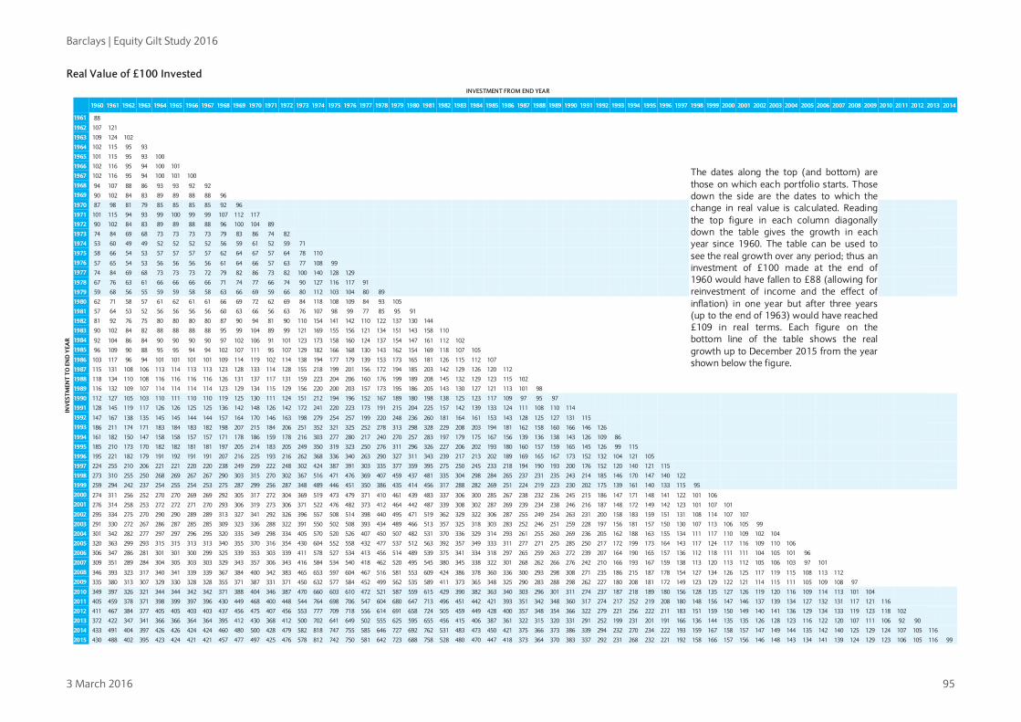
Barclays | Equity Gilt Study 2016
3 March 2016 95
Real Value of £100 Invested INVESTMENT FROM END YEAR
INV
ESTM
ENT
TO E
ND
YEA
R
1960 1961 1962 1963 1964 1965 1966 1967 1968 1969 1970 1971 1972 1973 1974 1975 1976 1977 1978 1979 1980 1981 1982 1983 1984 1985 1986 1987 1988 1989 1990 1991 1992 1993 1994 1995 1996 1997 1998 1999 2000 2001 2002 2003 2004 2005 2006 2007 2008 2009 2010 2011 2012 2013 2014
1961 88
1962 107 121
1963 109 124 102
1964 102 115 95 93
1965 101 115 95 93 100
1966 102 116 95 94 100 101 The dates along the top (and bottom) are
those on which each portfolio starts. Those down the side are the dates to which the change in real value is calculated. Reading the top figure in each column diagonally down the table gives the growth in each year since 1960. The table can be used to see the real growth over any period; thus an investment of £100 made at the end of 1960 would have fallen to £88 (allowing for reinvestment of income and the effect of inflation) in one year but after three years (up to the end of 1963) would have reached £109 in real terms. Each figure on the bottom line of the table shows the real growth up to December 2015 from the year shown below the figure.
1967 102 116 95 94 100 101 100
1968 94 107 88 86 93 93 92 92
1969 90 102 84 83 89 89 88 88 96
1970 87 98 81 79 85 85 85 85 92 96
1971 101 115 94 93 99 100 99 99 107 112 117
1972 90 102 84 83 89 89 88 88 96 100 104 89
1973 74 84 69 68 73 73 73 73 79 83 86 74 82
1974 53 60 49 49 52 52 52 52 56 59 61 52 59 71
1975 58 66 54 53 57 57 57 57 62 64 67 57 64 78 110
1976 57 65 54 53 56 56 56 56 61 64 66 57 63 77 108 99
1977 74 84 69 68 73 73 73 72 79 82 86 73 82 100 140 128 129
1978 67 76 63 61 66 66 66 66 71 74 77 66 74 90 127 116 117 91
1979 59 68 56 55 59 59 58 58 63 66 69 59 66 80 112 103 104 80 89
1980 62 71 58 57 61 62 61 61 66 69 72 62 69 84 118 108 109 84 93 105
1981 57 64 53 52 56 56 56 56 60 63 66 56 63 76 107 98 99 77 85 95 91
1982 81 92 76 75 80 80 80 80 87 90 94 81 90 110 154 141 142 110 122 137 130 144
1983 90 102 84 82 88 88 88 88 95 99 104 89 99 121 169 155 156 121 134 151 143 158 110
1984 92 104 86 84 90 90 90 90 97 102 106 91 101 123 173 158 160 124 137 154 147 161 112 102
1985 96 109 90 88 95 95 94 94 102 107 111 95 107 129 182 166 168 130 143 162 154 169 118 107 105
1986 103 117 96 94 101 101 101 101 109 114 119 102 114 138 194 177 179 139 153 173 165 181 126 115 112 107
1987 115 131 108 106 113 114 113 113 123 128 133 114 128 155 218 199 201 156 172 194 185 203 142 129 126 120 112
1988 118 134 110 108 116 116 116 116 126 131 137 117 131 159 223 204 206 160 176 199 189 208 145 132 129 123 115 102
1989 116 132 109 107 114 114 114 114 123 129 134 115 129 156 220 200 203 157 173 195 186 205 143 130 127 121 113 101 98
1990 112 127 105 103 110 111 110 110 119 125 130 111 124 151 212 194 196 152 167 189 180 198 138 125 123 117 109 97 95 97
1991 128 145 119 117 126 126 125 125 136 142 148 126 142 172 241 220 223 173 191 215 204 225 157 142 139 133 124 111 108 110 114
1992 147 167 138 135 145 145 144 144 157 164 170 146 163 198 279 254 257 199 220 248 236 260 181 164 161 153 143 128 125 127 131 115
1993 186 211 174 171 183 184 183 182 198 207 215 184 206 251 352 321 325 252 278 313 298 328 229 208 203 194 181 162 158 160 166 146 126
1994 161 182 150 147 158 158 157 157 171 178 186 159 178 216 303 277 280 217 240 270 257 283 197 179 175 167 156 139 136 138 143 126 109 86
1995 185 210 173 170 182 182 181 181 197 205 214 183 205 249 350 319 323 250 276 311 296 326 227 206 202 193 180 160 157 159 165 145 126 99 115
1996 195 221 182 179 191 192 191 191 207 216 225 193 216 262 368 336 340 263 290 327 311 343 239 217 213 202 189 169 165 167 173 152 132 104 121 105
1997 224 255 210 206 221 221 220 220 238 249 259 222 248 302 424 387 391 303 335 377 359 395 275 250 245 233 218 194 190 193 200 176 152 120 140 121 115
1998 273 310 255 250 268 269 267 267 290 303 315 270 302 367 516 471 476 369 407 459 437 481 335 304 298 284 265 237 231 235 243 214 185 146 170 147 140 122
1999 259 294 242 237 254 255 254 253 275 287 299 256 287 348 489 446 451 350 386 435 414 456 317 288 282 269 251 224 219 223 230 202 175 139 161 140 133 115 95
2000 274 311 256 252 270 270 269 269 292 305 317 272 304 369 519 473 479 371 410 461 439 483 337 306 300 285 267 238 232 236 245 215 186 147 171 148 141 122 101 106
2001 276 314 258 253 272 272 271 270 293 306 319 273 306 371 522 476 482 373 412 464 442 487 339 308 302 287 269 239 234 238 246 216 187 148 172 149 142 123 101 107 101
2002 295 334 275 270 290 290 289 289 313 327 341 292 326 396 557 508 514 398 440 495 471 519 362 329 322 306 287 255 249 254 263 231 200 158 183 159 151 131 108 114 107 107
2003 291 330 272 267 286 287 285 285 309 323 336 288 322 391 550 502 508 393 434 489 466 513 357 325 318 303 283 252 246 251 259 228 197 156 181 157 150 130 107 113 106 105 99
2004 301 342 282 277 297 297 296 295 320 335 349 298 334 405 570 520 526 407 450 507 482 531 370 336 329 314 293 261 255 260 269 236 205 162 188 163 155 134 111 117 110 109 102 104
2005 320 363 299 293 315 315 313 313 340 355 370 316 354 430 604 552 558 432 477 537 512 563 392 357 349 333 311 277 271 275 285 250 217 172 199 173 164 143 117 124 117 116 109 110 106
2006 306 347 286 281 301 301 300 299 325 339 353 303 339 411 578 527 534 413 456 514 489 539 375 341 334 318 297 265 259 263 272 239 207 164 190 165 157 136 112 118 111 111 104 105 101 96
2007 309 351 289 284 304 305 303 303 329 343 357 306 343 416 584 534 540 418 462 520 495 545 380 345 338 322 301 268 262 266 276 242 210 166 193 167 159 138 113 120 113 112 105 106 103 97 101
2008 346 393 323 317 340 341 339 339 367 384 400 342 383 465 653 597 604 467 516 581 553 609 424 386 378 360 336 300 293 298 308 271 235 186 215 187 178 154 127 134 126 125 117 119 115 108 113 112
2009 335 380 313 307 329 330 328 328 355 371 387 331 371 450 632 577 584 452 499 562 535 589 411 373 365 348 325 290 283 288 298 262 227 180 208 181 172 149 123 129 122 121 114 115 111 105 109 108 97
2010 349 397 326 321 344 344 342 342 371 388 404 346 387 470 660 603 610 472 521 587 559 615 429 390 382 363 340 303 296 301 311 274 237 187 218 189 180 156 128 135 127 126 119 120 116 109 114 113 101 104
2011 405 459 378 371 398 399 397 396 430 449 468 400 448 544 764 698 706 547 604 680 647 713 496 451 442 421 393 351 342 348 360 317 274 217 252 219 208 180 148 156 147 146 137 139 134 127 132 131 117 121 116
2012 411 467 384 377 405 405 403 403 437 456 475 407 456 553 777 709 718 556 614 691 658 724 505 459 449 428 400 357 348 354 366 322 279 221 256 222 211 183 151 159 150 149 140 141 136 129 134 133 119 123 118 102
2013 372 422 347 341 366 366 364 364 395 412 430 368 412 500 702 641 649 502 555 625 595 655 456 415 406 387 361 322 315 320 331 291 252 199 231 201 191 166 136 144 135 135 126 128 123 116 122 120 107 111 106 92 90
2014 433 491 404 397 426 426 424 424 460 480 500 428 479 582 818 747 755 585 646 727 692 762 531 483 473 450 421 375 366 373 386 339 294 232 270 234 222 193 159 167 158 157 147 149 144 135 142 140 125 129 124 107 105 116
2015 430 488 402 395 423 424 421 421 457 477 497 425 476 578 812 742 750 581 642 723 688 758 528 480 470 447 418 373 364 370 383 337 292 231 268 232 221 192 158 166 157 156 146 148 143 134 141 139 124 129 123 106 105 116 99
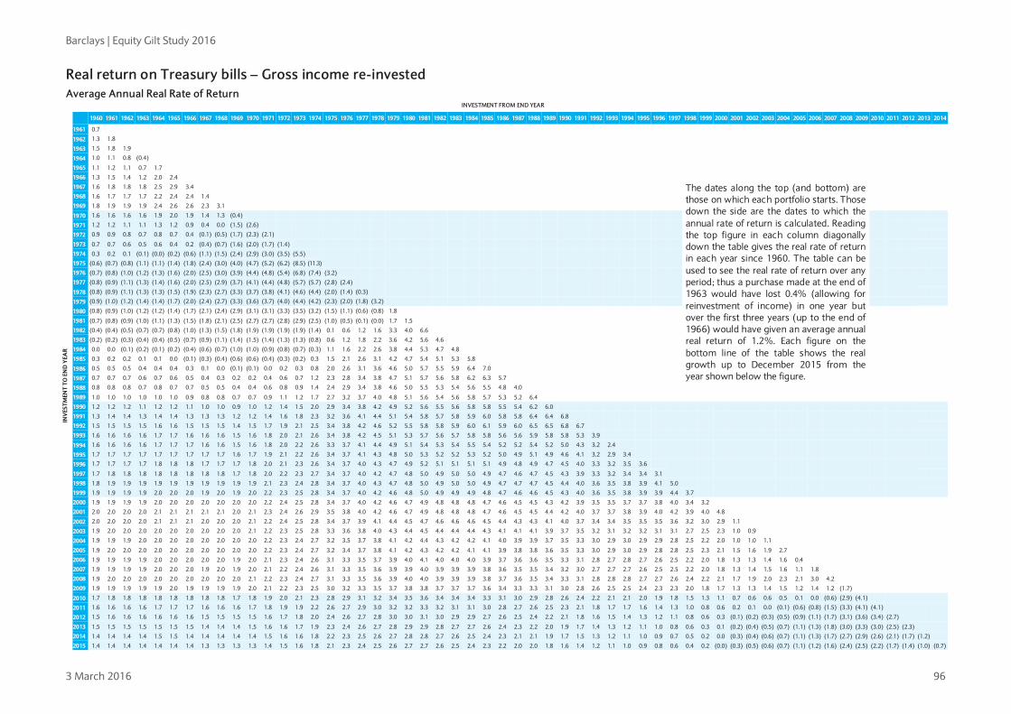
Barclays | Equity Gilt Study 2016
3 March 2016 96
Real return on Treasury bills – Gross income re-invested Average Annual Real Rate of Return
INVESTMENT FROM END YEAR
INV
ESTM
ENT
TO E
ND
YEA
R
1960 1961 1962 1963 1964 1965 1966 1967 1968 1969 1970 1971 1972 1973 1974 1975 1976 1977 1978 1979 1980 1981 1982 1983 1984 1985 1986 1987 1988 1989 1990 1991 1992 1993 1994 1995 1996 1997 1998 1999 2000 2001 2002 2003 2004 2005 2006 2007 2008 2009 2010 2011 2012 2013 2014
1961 0.7
1962 1.3 1.8
1963 1.5 1.8 1.9
1964 1.0 1.1 0.8 (0.4)
1965 1.1 1.2 1.1 0.7 1.7
1966 1.3 1.5 1.4 1.2 2.0 2.4 The dates along the top (and bottom) are
those on which each portfolio starts. Those down the side are the dates to which the annual rate of return is calculated. Reading the top figure in each column diagonally down the table gives the real rate of return in each year since 1960. The table can be used to see the real rate of return over any period; thus a purchase made at the end of 1963 would have lost 0.4% (allowing for reinvestment of income) in one year but over the first three years (up to the end of 1966) would have given an average annual real return of 1.2%. Each figure on the bottom line of the table shows the real growth up to December 2015 from the year shown below the figure.
1967 1.6 1.8 1.8 1.8 2.5 2.9 3.4
1968 1.6 1.7 1.7 1.7 2.2 2.4 2.4 1.4
1969 1.8 1.9 1.9 1.9 2.4 2.6 2.6 2.3 3.1
1970 1.6 1.6 1.6 1.6 1.9 2.0 1.9 1.4 1.3 (0.4)
1971 1.2 1.2 1.1 1.1 1.3 1.2 0.9 0.4 0.0 (1.5) (2.6)
1972 0.9 0.9 0.8 0.7 0.8 0.7 0.4 (0.1) (0.5) (1.7) (2.3) (2.1)
1973 0.7 0.7 0.6 0.5 0.6 0.4 0.2 (0.4) (0.7) (1.6) (2.0) (1.7) (1.4)
1974 0.3 0.2 0.1 (0.1) (0.0) (0.2) (0.6) (1.1) (1.5) (2.4) (2.9) (3.0) (3.5) (5.5)
1975 (0.6) (0.7) (0.8) (1.1) (1.1) (1.4) (1.8) (2.4) (3.0) (4.0) (4.7) (5.2) (6.2) (8.5) (11.3)
1976 (0.7) (0.8) (1.0) (1.2) (1.3) (1.6) (2.0) (2.5) (3.0) (3.9) (4.4) (4.8) (5.4) (6.8) (7.4) (3.2)
1977 (0.8) (0.9) (1.1) (1.3) (1.4) (1.6) (2.0) (2.5) (2.9) (3.7) (4.1) (4.4) (4.8) (5.7) (5.7) (2.8) (2.4)
1978 (0.8) (0.9) (1.1) (1.3) (1.3) (1.5) (1.9) (2.3) (2.7) (3.3) (3.7) (3.8) (4.1) (4.6) (4.4) (2.0) (1.4) (0.3)
1979 (0.9) (1.0) (1.2) (1.4) (1.4) (1.7) (2.0) (2.4) (2.7) (3.3) (3.6) (3.7) (4.0) (4.4) (4.2) (2.3) (2.0) (1.8) (3.2)
1980 (0.8) (0.9) (1.0) (1.2) (1.2) (1.4) (1.7) (2.1) (2.4) (2.9) (3.1) (3.1) (3.3) (3.5) (3.2) (1.5) (1.1) (0.6) (0.8) 1.8
1981 (0.7) (0.8) (0.9) (1.0) (1.1) (1.3) (1.5) (1.8) (2.1) (2.5) (2.7) (2.7) (2.8) (2.9) (2.5) (1.0) (0.5) (0.1) (0.0) 1.7 1.5
1982 (0.4) (0.4) (0.5) (0.7) (0.7) (0.8) (1.0) (1.3) (1.5) (1.8) (1.9) (1.9) (1.9) (1.9) (1.4) 0.1 0.6 1.2 1.6 3.3 4.0 6.6
1983 (0.2) (0.2) (0.3) (0.4) (0.4) (0.5) (0.7) (0.9) (1.1) (1.4) (1.5) (1.4) (1.3) (1.3) (0.8) 0.6 1.2 1.8 2.2 3.6 4.2 5.6 4.6
1984 0.0 0.0 (0.1) (0.2) (0.1) (0.2) (0.4) (0.6) (0.7) (1.0) (1.0) (0.9) (0.8) (0.7) (0.3) 1.1 1.6 2.2 2.6 3.8 4.4 5.3 4.7 4.8
1985 0.3 0.2 0.2 0.1 0.1 0.0 (0.1) (0.3) (0.4) (0.6) (0.6) (0.4) (0.3) (0.2) 0.3 1.5 2.1 2.6 3.1 4.2 4.7 5.4 5.1 5.3 5.8
1986 0.5 0.5 0.5 0.4 0.4 0.4 0.3 0.1 0.0 (0.1) (0.1) 0.0 0.2 0.3 0.8 2.0 2.6 3.1 3.6 4.6 5.0 5.7 5.5 5.9 6.4 7.0
1987 0.7 0.7 0.7 0.6 0.7 0.6 0.5 0.4 0.3 0.2 0.2 0.4 0.6 0.7 1.2 2.3 2.8 3.4 3.8 4.7 5.1 5.7 5.6 5.8 6.2 6.3 5.7
1988 0.8 0.8 0.8 0.7 0.8 0.7 0.7 0.5 0.5 0.4 0.4 0.6 0.8 0.9 1.4 2.4 2.9 3.4 3.8 4.6 5.0 5.5 5.3 5.4 5.6 5.5 4.8 4.0
1989 1.0 1.0 1.0 1.0 1.0 1.0 0.9 0.8 0.8 0.7 0.7 0.9 1.1 1.2 1.7 2.7 3.2 3.7 4.0 4.8 5.1 5.6 5.4 5.6 5.8 5.7 5.3 5.2 6.4
1990 1.2 1.2 1.2 1.1 1.2 1.2 1.1 1.0 1.0 0.9 1.0 1.2 1.4 1.5 2.0 2.9 3.4 3.8 4.2 4.9 5.2 5.6 5.5 5.6 5.8 5.8 5.5 5.4 6.2 6.0
1991 1.3 1.4 1.4 1.3 1.4 1.4 1.3 1.3 1.3 1.2 1.2 1.4 1.6 1.8 2.3 3.2 3.6 4.1 4.4 5.1 5.4 5.8 5.7 5.8 5.9 6.0 5.8 5.8 6.4 6.4 6.8
1992 1.5 1.5 1.5 1.5 1.6 1.6 1.5 1.5 1.5 1.4 1.5 1.7 1.9 2.1 2.5 3.4 3.8 4.2 4.6 5.2 5.5 5.8 5.8 5.9 6.0 6.1 5.9 6.0 6.5 6.5 6.8 6.7
1993 1.6 1.6 1.6 1.6 1.7 1.7 1.6 1.6 1.6 1.5 1.6 1.8 2.0 2.1 2.6 3.4 3.8 4.2 4.5 5.1 5.3 5.7 5.6 5.7 5.8 5.8 5.6 5.6 5.9 5.8 5.8 5.3 3.9
1994 1.6 1.6 1.6 1.6 1.7 1.7 1.7 1.6 1.6 1.5 1.6 1.8 2.0 2.2 2.6 3.3 3.7 4.1 4.4 4.9 5.1 5.4 5.3 5.4 5.5 5.4 5.2 5.2 5.4 5.2 5.0 4.3 3.2 2.4
1995 1.7 1.7 1.7 1.7 1.7 1.7 1.7 1.7 1.7 1.6 1.7 1.9 2.1 2.2 2.6 3.4 3.7 4.1 4.3 4.8 5.0 5.3 5.2 5.2 5.3 5.2 5.0 4.9 5.1 4.9 4.6 4.1 3.2 2.9 3.4
1996 1.7 1.7 1.7 1.7 1.8 1.8 1.8 1.7 1.7 1.7 1.8 2.0 2.1 2.3 2.6 3.4 3.7 4.0 4.3 4.7 4.9 5.2 5.1 5.1 5.1 5.1 4.9 4.8 4.9 4.7 4.5 4.0 3.3 3.2 3.5 3.6
1997 1.7 1.8 1.8 1.8 1.8 1.8 1.8 1.8 1.8 1.7 1.8 2.0 2.2 2.3 2.7 3.4 3.7 4.0 4.2 4.7 4.8 5.0 4.9 5.0 5.0 4.9 4.7 4.6 4.7 4.5 4.3 3.9 3.3 3.2 3.4 3.4 3.1
1998 1.8 1.9 1.9 1.9 1.9 1.9 1.9 1.9 1.9 1.9 1.9 2.1 2.3 2.4 2.8 3.4 3.7 4.0 4.3 4.7 4.8 5.0 4.9 5.0 5.0 4.9 4.7 4.7 4.7 4.5 4.4 4.0 3.6 3.5 3.8 3.9 4.1 5.0
1999 1.9 1.9 1.9 1.9 2.0 2.0 2.0 1.9 2.0 1.9 2.0 2.2 2.3 2.5 2.8 3.4 3.7 4.0 4.2 4.6 4.8 5.0 4.9 4.9 4.9 4.8 4.7 4.6 4.6 4.5 4.3 4.0 3.6 3.5 3.8 3.9 3.9 4.4 3.7
2000 1.9 1.9 1.9 1.9 2.0 2.0 2.0 2.0 2.0 2.0 2.0 2.2 2.4 2.5 2.8 3.4 3.7 4.0 4.2 4.6 4.7 4.9 4.8 4.8 4.8 4.7 4.6 4.5 4.5 4.3 4.2 3.9 3.5 3.5 3.7 3.7 3.8 4.0 3.4 3.2
2001 2.0 2.0 2.0 2.0 2.1 2.1 2.1 2.1 2.1 2.0 2.1 2.3 2.4 2.6 2.9 3.5 3.8 4.0 4.2 4.6 4.7 4.9 4.8 4.8 4.8 4.7 4.6 4.5 4.5 4.4 4.2 4.0 3.7 3.7 3.8 3.9 4.0 4.2 3.9 4.0 4.8
2002 2.0 2.0 2.0 2.0 2.1 2.1 2.1 2.0 2.0 2.0 2.1 2.2 2.4 2.5 2.8 3.4 3.7 3.9 4.1 4.4 4.5 4.7 4.6 4.6 4.6 4.5 4.4 4.3 4.3 4.1 4.0 3.7 3.4 3.4 3.5 3.5 3.5 3.6 3.2 3.0 2.9 1.1
2003 1.9 2.0 2.0 2.0 2.0 2.0 2.0 2.0 2.0 2.0 2.1 2.2 2.3 2.5 2.8 3.3 3.6 3.8 4.0 4.3 4.4 4.5 4.4 4.4 4.4 4.3 4.1 4.1 4.1 3.9 3.7 3.5 3.2 3.1 3.2 3.2 3.1 3.1 2.7 2.5 2.3 1.0 0.9
2004 1.9 1.9 1.9 2.0 2.0 2.0 2.0 2.0 2.0 2.0 2.0 2.2 2.3 2.4 2.7 3.2 3.5 3.7 3.8 4.1 4.2 4.4 4.3 4.2 4.2 4.1 4.0 3.9 3.9 3.7 3.5 3.3 3.0 2.9 3.0 2.9 2.9 2.8 2.5 2.2 2.0 1.0 1.0 1.1
2005 1.9 2.0 2.0 2.0 2.0 2.0 2.0 2.0 2.0 2.0 2.0 2.2 2.3 2.4 2.7 3.2 3.4 3.7 3.8 4.1 4.2 4.3 4.2 4.2 4.1 4.1 3.9 3.8 3.8 3.6 3.5 3.3 3.0 2.9 3.0 2.9 2.8 2.8 2.5 2.3 2.1 1.5 1.6 1.9 2.7
2006 1.9 1.9 1.9 1.9 2.0 2.0 2.0 2.0 2.0 1.9 2.0 2.1 2.3 2.4 2.6 3.1 3.3 3.5 3.7 3.9 4.0 4.1 4.0 4.0 4.0 3.9 3.7 3.6 3.6 3.5 3.3 3.1 2.8 2.7 2.8 2.7 2.6 2.5 2.2 2.0 1.8 1.3 1.3 1.4 1.6 0.4
2007 1.9 1.9 1.9 1.9 2.0 2.0 2.0 1.9 2.0 1.9 2.0 2.1 2.2 2.4 2.6 3.1 3.3 3.5 3.6 3.9 3.9 4.0 3.9 3.9 3.9 3.8 3.6 3.5 3.5 3.4 3.2 3.0 2.7 2.7 2.7 2.6 2.5 2.5 2.2 2.0 1.8 1.3 1.4 1.5 1.6 1.1 1.8
2008 1.9 2.0 2.0 2.0 2.0 2.0 2.0 2.0 2.0 2.0 2.1 2.2 2.3 2.4 2.7 3.1 3.3 3.5 3.6 3.9 4.0 4.0 3.9 3.9 3.9 3.8 3.7 3.6 3.5 3.4 3.3 3.1 2.8 2.8 2.8 2.7 2.7 2.6 2.4 2.2 2.1 1.7 1.9 2.0 2.3 2.1 3.0 4.2
2009 1.9 1.9 1.9 1.9 1.9 2.0 1.9 1.9 1.9 1.9 2.0 2.1 2.2 2.3 2.5 3.0 3.2 3.3 3.5 3.7 3.8 3.8 3.7 3.7 3.7 3.6 3.4 3.3 3.3 3.1 3.0 2.8 2.6 2.5 2.5 2.4 2.3 2.3 2.0 1.8 1.7 1.3 1.3 1.4 1.5 1.2 1.4 1.2 (1.7)
2010 1.7 1.8 1.8 1.8 1.8 1.8 1.8 1.8 1.8 1.7 1.8 1.9 2.0 2.1 2.3 2.8 2.9 3.1 3.2 3.4 3.5 3.6 3.4 3.4 3.4 3.3 3.1 3.0 2.9 2.8 2.6 2.4 2.2 2.1 2.1 2.0 1.9 1.8 1.5 1.3 1.1 0.7 0.6 0.6 0.5 0.1 0.0 (0.6) (2.9) (4.1)
2011 1.6 1.6 1.6 1.6 1.7 1.7 1.7 1.6 1.6 1.6 1.7 1.8 1.9 1.9 2.2 2.6 2.7 2.9 3.0 3.2 3.2 3.3 3.2 3.1 3.1 3.0 2.8 2.7 2.6 2.5 2.3 2.1 1.8 1.7 1.7 1.6 1.4 1.3 1.0 0.8 0.6 0.2 0.1 0.0 (0.1) (0.6) (0.8) (1.5) (3.3) (4.1) (4.1)
2012 1.5 1.6 1.6 1.6 1.6 1.6 1.6 1.5 1.5 1.5 1.5 1.6 1.7 1.8 2.0 2.4 2.6 2.7 2.8 3.0 3.0 3.1 3.0 2.9 2.9 2.7 2.6 2.5 2.4 2.2 2.1 1.8 1.6 1.5 1.4 1.3 1.2 1.1 0.8 0.6 0.3 (0.1) (0.2) (0.3) (0.5) (0.9) (1.1) (1.7) (3.1) (3.6) (3.4) (2.7)
2013 1.5 1.5 1.5 1.5 1.5 1.5 1.5 1.4 1.4 1.4 1.5 1.6 1.6 1.7 1.9 2.3 2.4 2.6 2.7 2.8 2.9 2.9 2.8 2.7 2.7 2.6 2.4 2.3 2.2 2.0 1.9 1.7 1.4 1.3 1.2 1.1 1.0 0.8 0.6 0.3 0.1 (0.2) (0.4) (0.5) (0.7) (1.1) (1.3) (1.8) (3.0) (3.3) (3.0) (2.5) (2.3)
2014 1.4 1.4 1.4 1.4 1.5 1.5 1.4 1.4 1.4 1.4 1.4 1.5 1.6 1.6 1.8 2.2 2.3 2.5 2.6 2.7 2.8 2.8 2.7 2.6 2.5 2.4 2.3 2.1 2.1 1.9 1.7 1.5 1.3 1.2 1.1 1.0 0.9 0.7 0.5 0.2 0.0 (0.3) (0.4) (0.6) (0.7) (1.1) (1.3) (1.7) (2.7) (2.9) (2.6) (2.1) (1.7) (1.2)
2015 1.4 1.4 1.4 1.4 1.4 1.4 1.4 1.3 1.3 1.3 1.3 1.4 1.5 1.6 1.8 2.1 2.3 2.4 2.5 2.6 2.7 2.7 2.6 2.5 2.4 2.3 2.2 2.0 2.0 1.8 1.6 1.4 1.2 1.1 1.0 0.9 0.8 0.6 0.4 0.2 (0.0) (0.3) (0.5) (0.6) (0.7) (1.1) (1.2) (1.6) (2.4) (2.5) (2.2) (1.7) (1.4) (1.0) (0.7)

Barclays | Equity Gilt Study 2016
3 March 2016 97
Real Value of £100 Invested INVESTMENT FROM END YEAR
INV
ESTM
ENT
TO E
ND
YEA
R
1960 1961 1962 1963 1964 1965 1966 1967 1968 1969 1970 1971 1972 1973 1974 1975 1976 1977 1978 1979 1980 1981 1982 1983 1984 1985 1986 1987 1988 1989 1990 1991 1992 1993 1994 1995 1996 1997 1998 1999 2000 2001 2002 2003 2004 2005 2006 2007 2008 2009 2010 2011 2012 2013 2014
1961 88
1962 107 121
1963 109 124 102
1964 102 115 95 93
1965 101 115 95 93 100
1966 102 116 95 94 100 101 The dates along the top (and bottom) are
those on which each portfolio starts. Those down the side are the dates to which the change in real value is calculated. Reading the top figure in each column diagonally down the table gives the growth in each year since 1960. The table can be used to see the real growth over any period; thus an investment of £100 made at the end of 1960 would have fallen to £88 (allowing for reinvestment of income and the effect of inflation) in one year but after three years (up to the end of 1963) would have reached £109 in real terms. Each figure on the bottom line of the table shows the real growth up to December 2015 from the year shown below the figure.
1967 102 116 95 94 100 101 100
1968 94 107 88 86 93 93 92 92
1969 90 102 84 83 89 89 88 88 96
1970 87 98 81 79 85 85 85 85 92 96
1971 101 115 94 93 99 100 99 99 107 112 117
1972 90 102 84 83 89 89 88 88 96 100 104 89
1973 74 84 69 68 73 73 73 73 79 83 86 74 82
1974 53 60 49 49 52 52 52 52 56 59 61 52 59 71
1975 58 66 54 53 57 57 57 57 62 64 67 57 64 78 110
1976 57 65 54 53 56 56 56 56 61 64 66 57 63 77 108 99
1977 74 84 69 68 73 73 73 72 79 82 86 73 82 100 140 128 129
1978 67 76 63 61 66 66 66 66 71 74 77 66 74 90 127 116 117 91
1979 59 68 56 55 59 59 58 58 63 66 69 59 66 80 112 103 104 80 89
1980 62 71 58 57 61 62 61 61 66 69 72 62 69 84 118 108 109 84 93 105
1981 57 64 53 52 56 56 56 56 60 63 66 56 63 76 107 98 99 77 85 95 91
1982 81 92 76 75 80 80 80 80 87 90 94 81 90 110 154 141 142 110 122 137 130 144
1983 90 102 84 82 88 88 88 88 95 99 104 89 99 121 169 155 156 121 134 151 143 158 110
1984 92 104 86 84 90 90 90 90 97 102 106 91 101 123 173 158 160 124 137 154 147 161 112 102
1985 96 109 90 88 95 95 94 94 102 107 111 95 107 129 182 166 168 130 143 162 154 169 118 107 105
1986 103 117 96 94 101 101 101 101 109 114 119 102 114 138 194 177 179 139 153 173 165 181 126 115 112 107
1987 115 131 108 106 113 114 113 113 123 128 133 114 128 155 218 199 201 156 172 194 185 203 142 129 126 120 112
1988 118 134 110 108 116 116 116 116 126 131 137 117 131 159 223 204 206 160 176 199 189 208 145 132 129 123 115 102
1989 116 132 109 107 114 114 114 114 123 129 134 115 129 156 220 200 203 157 173 195 186 205 143 130 127 121 113 101 98
1990 112 127 105 103 110 111 110 110 119 125 130 111 124 151 212 194 196 152 167 189 180 198 138 125 123 117 109 97 95 97
1991 128 145 119 117 126 126 125 125 136 142 148 126 142 172 241 220 223 173 191 215 204 225 157 142 139 133 124 111 108 110 114
1992 147 167 138 135 145 145 144 144 157 164 170 146 163 198 279 254 257 199 220 248 236 260 181 164 161 153 143 128 125 127 131 115
1993 186 211 174 171 183 184 183 182 198 207 215 184 206 251 352 321 325 252 278 313 298 328 229 208 203 194 181 162 158 160 166 146 126
1994 161 182 150 147 158 158 157 157 171 178 186 159 178 216 303 277 280 217 240 270 257 283 197 179 175 167 156 139 136 138 143 126 109 86
1995 185 210 173 170 182 182 181 181 197 205 214 183 205 249 350 319 323 250 276 311 296 326 227 206 202 193 180 160 157 159 165 145 126 99 115
1996 195 221 182 179 191 192 191 191 207 216 225 193 216 262 368 336 340 263 290 327 311 343 239 217 213 202 189 169 165 167 173 152 132 104 121 105
1997 224 255 210 206 221 221 220 220 238 249 259 222 248 302 424 387 391 303 335 377 359 395 275 250 245 233 218 194 190 193 200 176 152 120 140 121 115
1998 273 310 255 250 268 269 267 267 290 303 315 270 302 367 516 471 476 369 407 459 437 481 335 304 298 284 265 237 231 235 243 214 185 146 170 147 140 122
1999 259 294 242 237 254 255 254 253 275 287 299 256 287 348 489 446 451 350 386 435 414 456 317 288 282 269 251 224 219 223 230 202 175 139 161 140 133 115 95
2000 274 311 256 252 270 270 269 269 292 305 317 272 304 369 519 473 479 371 410 461 439 483 337 306 300 285 267 238 232 236 245 215 186 147 171 148 141 122 101 106
2001 276 314 258 253 272 272 271 270 293 306 319 273 306 371 522 476 482 373 412 464 442 487 339 308 302 287 269 239 234 238 246 216 187 148 172 149 142 123 101 107 101
2002 295 334 275 270 290 290 289 289 313 327 341 292 326 396 557 508 514 398 440 495 471 519 362 329 322 306 287 255 249 254 263 231 200 158 183 159 151 131 108 114 107 107
2003 291 330 272 267 286 287 285 285 309 323 336 288 322 391 550 502 508 393 434 489 466 513 357 325 318 303 283 252 246 251 259 228 197 156 181 157 150 130 107 113 106 105 99
2004 301 342 282 277 297 297 296 295 320 335 349 298 334 405 570 520 526 407 450 507 482 531 370 336 329 314 293 261 255 260 269 236 205 162 188 163 155 134 111 117 110 109 102 104
2005 320 363 299 293 315 315 313 313 340 355 370 316 354 430 604 552 558 432 477 537 512 563 392 357 349 333 311 277 271 275 285 250 217 172 199 173 164 143 117 124 117 116 109 110 106
2006 306 347 286 281 301 301 300 299 325 339 353 303 339 411 578 527 534 413 456 514 489 539 375 341 334 318 297 265 259 263 272 239 207 164 190 165 157 136 112 118 111 111 104 105 101 96
2007 309 351 289 284 304 305 303 303 329 343 357 306 343 416 584 534 540 418 462 520 495 545 380 345 338 322 301 268 262 266 276 242 210 166 193 167 159 138 113 120 113 112 105 106 103 97 101
2008 346 393 323 317 340 341 339 339 367 384 400 342 383 465 653 597 604 467 516 581 553 609 424 386 378 360 336 300 293 298 308 271 235 186 215 187 178 154 127 134 126 125 117 119 115 108 113 112
2009 335 380 313 307 329 330 328 328 355 371 387 331 371 450 632 577 584 452 499 562 535 589 411 373 365 348 325 290 283 288 298 262 227 180 208 181 172 149 123 129 122 121 114 115 111 105 109 108 97
2010 349 397 326 321 344 344 342 342 371 388 404 346 387 470 660 603 610 472 521 587 559 615 429 390 382 363 340 303 296 301 311 274 237 187 218 189 180 156 128 135 127 126 119 120 116 109 114 113 101 104
2011 405 459 378 371 398 399 397 396 430 449 468 400 448 544 764 698 706 547 604 680 647 713 496 451 442 421 393 351 342 348 360 317 274 217 252 219 208 180 148 156 147 146 137 139 134 127 132 131 117 121 116
2012 411 467 384 377 405 405 403 403 437 456 475 407 456 553 777 709 718 556 614 691 658 724 505 459 449 428 400 357 348 354 366 322 279 221 256 222 211 183 151 159 150 149 140 141 136 129 134 133 119 123 118 102
2013 372 422 347 341 366 366 364 364 395 412 430 368 412 500 702 641 649 502 555 625 595 655 456 415 406 387 361 322 315 320 331 291 252 199 231 201 191 166 136 144 135 135 126 128 123 116 122 120 107 111 106 92 90
2014 433 491 404 397 426 426 424 424 460 480 500 428 479 582 818 747 755 585 646 727 692 762 531 483 473 450 421 375 366 373 386 339 294 232 270 234 222 193 159 167 158 157 147 149 144 135 142 140 125 129 124 107 105 116
2015 430 488 402 395 423 424 421 421 457 477 497 425 476 578 812 742 750 581 642 723 688 758 528 480 470 447 418 373 364 370 383 337 292 231 268 232 221 192 158 166 157 156 146 148 143 134 141 139 124 129 123 106 105 116 99
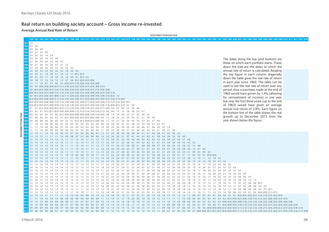
Barclays | Equity Gilt Study 2016
3 March 2016 98
Real return on building society account – Gross income re-invested Average Annual Real Rate of Return
INVESTMENT FROM END YEAR
INV
ESTM
ENT
TO E
ND
YEA
R
1960 1961 1962 1963 1964 1965 1966 1967 1968 1969 1970 1971 1972 1973 1974 1975 1976 1977 1978 1979 1980 1981 1982 1983 1984 1985 1986 1987 1988 1989 1990 1991 1992 1993 1994 1995 1996 1997 1998 1999 2000 2001 2002 2003 2004 2005 2006 2007 2008 2009 2010 2011 2012 2013 2014
1961 1.4
1962 2.4 3.4
1963 2.9 3.6 3.9
1964 2.4 2.7 2.4 0.9
1965 2.3 2.5 2.2 1.4 1.9
1966 2.4 2.6 2.4 1.9 2.5 3.0
The dates along the top (and bottom) are those on which each portfolio starts. Those down the side are the dates to which the annual rate of return is calculated. Reading the top figure in each column diagonally down the table gives the real rate of return in each year since 1960. The table can be used to see the real rate of return over any period; thus a purchase made at the end of 1960 would have grown by 1.4% (allowing for reinvestment of income) in one year but over the first three years (up to the end of 1963) would have given an average annual real return of 2.9%. Each figure on the bottom line of the table shows the real growth up to December 2015 from the year shown below the figure.
1967 2.7 3.0 2.9 2.6 3.2 3.8 4.7
1968 2.6 2.7 2.6 2.4 2.8 3.1 3.1 1.5
1969 2.7 2.8 2.8 2.6 2.9 3.2 3.2 2.5 3.5
1970 2.5 2.6 2.5 2.3 2.5 2.6 2.5 1.8 2.0 0.6
1971 2.2 2.2 2.1 1.9 2.0 2.1 1.9 1.2 1.1 (0.1) (0.7)
1972 2.0 2.1 2.0 1.7 1.8 1.8 1.6 1.0 0.9 0.1 (0.1) 0.5
1973 1.8 1.8 1.7 1.5 1.6 1.5 1.3 0.7 0.6 (0.1) (0.3) (0.2) (0.8)
1974 1.2 1.1 1.0 0.7 0.7 0.6 0.2 (0.4) (0.7) (1.5) (2.0) (2.4) (3.8) (6.8)
1975 0.3 0.2 (0.0) (0.3) (0.4) (0.7) (1.1) (1.8) (2.2) (3.2) (3.9) (4.7) (6.3) (9.0) (11.1)
1976 0.0 (0.1) (0.3) (0.6) (0.7) (1.0) (1.4) (2.0) (2.4) (3.3) (3.9) (4.5) (5.7) (7.3) (7.6) (3.8)
1977 (0.0) (0.1) (0.4) (0.7) (0.8) (1.0) (1.4) (1.9) (2.3) (3.0) (3.5) (4.0) (4.8) (5.8) (5.5) (2.6) (1.3)
1978 0.0 (0.1) (0.3) (0.6) (0.7) (0.9) (1.2) (1.7) (2.0) (2.6) (3.0) (3.3) (3.9) (4.5) (3.9) (1.4) (0.2) 1.0
1979 (0.2) (0.3) (0.5) (0.8) (0.9) (1.1) (1.4) (1.9) (2.2) (2.8) (3.1) (3.4) (4.0) (4.5) (4.0) (2.1) (1.6) (1.7) (4.3)
1980 (0.2) (0.3) (0.5) (0.8) (0.9) (1.0) (1.3) (1.8) (2.0) (2.5) (2.8) (3.1) (3.5) (3.9) (3.4) (1.7) (1.2) (1.2) (2.2) (0.1)
1981 (0.2) (0.2) (0.4) (0.7) (0.8) (0.9) (1.2) (1.6) (1.8) (2.2) (2.5) (2.7) (3.0) (3.3) (2.8) (1.3) (0.8) (0.7) (1.2) 0.3 0.8
1982 0.1 0.1 (0.1) (0.3) (0.4) (0.5) (0.7) (1.1) (1.3) (1.6) (1.8) (1.9) (2.1) (2.3) (1.7) (0.3) 0.4 0.7 0.6 2.3 3.6 6.4
1983 0.3 0.2 0.1 (0.1) (0.1) (0.3) (0.4) (0.8) (0.9) (1.2) (1.3) (1.4) (1.6) (1.6) (1.1) 0.3 0.9 1.3 1.3 2.8 3.8 5.3 4.1
1984 0.5 0.5 0.3 0.2 0.1 0.0 (0.1) (0.4) (0.5) (0.8) (0.9) (0.9) (1.0) (1.0) (0.4) 0.8 1.4 1.8 2.0 3.2 4.1 5.2 4.6 5.2
1985 0.7 0.6 0.5 0.4 0.3 0.3 0.1 (0.1) (0.2) (0.5) (0.5) (0.5) (0.6) (0.6) 0.0 1.2 1.8 2.2 2.4 3.5 4.3 5.1 4.7 5.0 4.8
1986 0.9 0.9 0.8 0.6 0.6 0.6 0.4 0.2 0.1 (0.1) (0.1) (0.0) (0.1) (0.0) 0.6 1.7 2.3 2.7 2.9 3.9 4.6 5.4 5.2 5.5 5.7 6.6
1987 1.1 1.0 1.0 0.8 0.8 0.8 0.7 0.5 0.4 0.3 0.2 0.3 0.3 0.4 0.9 2.0 2.6 3.0 3.2 4.2 4.8 5.5 5.3 5.6 5.7 6.2 5.7
1988 1.1 1.1 1.0 0.9 0.9 0.8 0.7 0.5 0.5 0.3 0.3 0.4 0.4 0.4 1.0 2.0 2.5 2.8 3.0 3.9 4.4 4.9 4.6 4.7 4.6 4.5 3.5 1.4
1989 1.1 1.1 1.0 0.9 0.9 0.9 0.8 0.6 0.6 0.4 0.4 0.5 0.5 0.6 1.1 2.0 2.5 2.8 3.0 3.7 4.2 4.6 4.4 4.4 4.3 4.1 3.3 2.1 2.8
1990 1.2 1.2 1.1 1.0 1.0 1.0 0.9 0.7 0.7 0.5 0.5 0.6 0.6 0.7 1.2 2.1 2.5 2.8 2.9 3.6 4.0 4.4 4.1 4.1 4.0 3.8 3.1 2.2 2.6 2.5
1991 1.3 1.3 1.2 1.1 1.1 1.1 1.0 0.9 0.8 0.7 0.7 0.8 0.8 0.9 1.4 2.2 2.6 2.9 3.1 3.7 4.1 4.4 4.2 4.2 4.1 3.9 3.4 2.8 3.3 3.6 4.6
1992 1.5 1.5 1.4 1.3 1.3 1.3 1.2 1.1 1.1 1.0 1.0 1.1 1.1 1.2 1.7 2.5 2.9 3.2 3.3 4.0 4.3 4.6 4.4 4.5 4.4 4.3 4.0 3.6 4.2 4.6 5.7 6.8
1993 1.5 1.5 1.4 1.3 1.4 1.3 1.3 1.1 1.1 1.0 1.0 1.1 1.2 1.3 1.7 2.5 2.9 3.1 3.3 3.8 4.1 4.4 4.2 4.2 4.1 4.1 3.7 3.4 3.8 4.0 4.5 4.5 2.2
1994 1.5 1.5 1.4 1.3 1.3 1.3 1.3 1.1 1.1 1.0 1.0 1.1 1.1 1.2 1.7 2.4 2.7 3.0 3.1 3.6 3.9 4.1 3.9 3.9 3.8 3.7 3.3 3.0 3.3 3.4 3.6 3.2 1.5 0.8
1995 1.4 1.4 1.4 1.3 1.3 1.3 1.2 1.1 1.1 1.0 1.0 1.1 1.1 1.2 1.6 2.3 2.6 2.9 3.0 3.4 3.7 3.9 3.7 3.7 3.5 3.4 3.0 2.7 2.9 2.9 3.0 2.6 1.2 0.7 0.7
1996 1.4 1.4 1.3 1.3 1.3 1.3 1.2 1.1 1.1 1.0 1.0 1.1 1.1 1.2 1.5 2.2 2.5 2.7 2.8 3.2 3.4 3.6 3.4 3.4 3.2 3.1 2.7 2.4 2.5 2.5 2.5 2.1 0.9 0.5 0.4 0.2
1997 1.3 1.3 1.3 1.2 1.2 1.2 1.1 1.0 1.0 0.9 0.9 1.0 1.0 1.1 1.5 2.1 2.4 2.5 2.6 3.0 3.2 3.4 3.2 3.1 2.9 2.8 2.4 2.1 2.2 2.1 2.1 1.7 0.6 0.3 0.1 (0.2) (0.5)
1998 1.4 1.4 1.4 1.3 1.3 1.3 1.2 1.1 1.1 1.0 1.0 1.1 1.1 1.2 1.6 2.2 2.4 2.6 2.7 3.1 3.3 3.4 3.2 3.2 3.0 2.9 2.6 2.3 2.4 2.4 2.3 2.0 1.2 1.0 1.1 1.2 1.8 4.2
1999 1.5 1.5 1.4 1.3 1.4 1.3 1.3 1.2 1.2 1.1 1.1 1.2 1.2 1.3 1.6 2.2 2.5 2.6 2.7 3.1 3.3 3.4 3.2 3.2 3.0 2.9 2.6 2.4 2.5 2.4 2.4 2.2 1.5 1.4 1.5 1.8 2.3 3.7 3.3
2000 1.5 1.5 1.4 1.4 1.4 1.4 1.3 1.2 1.2 1.2 1.2 1.2 1.3 1.3 1.7 2.2 2.5 2.6 2.7 3.1 3.2 3.4 3.2 3.1 3.0 2.9 2.6 2.4 2.5 2.4 2.4 2.2 1.6 1.6 1.7 1.9 2.3 3.3 2.9 2.5
2001 1.6 1.6 1.5 1.4 1.5 1.4 1.4 1.3 1.3 1.2 1.3 1.3 1.4 1.4 1.8 2.3 2.5 2.7 2.8 3.1 3.3 3.4 3.2 3.2 3.1 3.0 2.7 2.5 2.6 2.6 2.6 2.4 1.9 1.9 2.0 2.2 2.7 3.5 3.3 3.2 4.0
2002 1.5 1.5 1.5 1.4 1.4 1.4 1.4 1.3 1.3 1.2 1.2 1.3 1.3 1.4 1.7 2.2 2.5 2.6 2.7 3.0 3.1 3.2 3.1 3.0 2.9 2.8 2.6 2.4 2.4 2.4 2.4 2.2 1.8 1.7 1.8 2.0 2.3 2.9 2.5 2.3 2.2 0.4
2003 1.5 1.5 1.5 1.4 1.4 1.4 1.4 1.3 1.3 1.2 1.2 1.3 1.3 1.4 1.7 2.2 2.4 2.5 2.6 2.9 3.0 3.1 3.0 2.9 2.8 2.7 2.5 2.2 2.3 2.3 2.3 2.1 1.6 1.6 1.7 1.8 2.0 2.5 2.1 1.8 1.6 0.5 0.5
2004 1.5 1.5 1.4 1.4 1.4 1.4 1.3 1.2 1.2 1.2 1.2 1.3 1.3 1.3 1.6 2.1 2.3 2.5 2.5 2.8 2.9 3.0 2.9 2.8 2.7 2.6 2.4 2.2 2.2 2.2 2.1 2.0 1.6 1.5 1.6 1.7 1.9 2.2 1.9 1.6 1.4 0.6 0.6 0.7
2005 1.5 1.5 1.4 1.4 1.4 1.4 1.3 1.3 1.3 1.2 1.2 1.3 1.3 1.4 1.6 2.1 2.3 2.4 2.5 2.8 2.9 3.0 2.8 2.8 2.6 2.5 2.3 2.1 2.2 2.1 2.1 1.9 1.6 1.5 1.6 1.7 1.8 2.2 1.9 1.6 1.5 0.8 1.0 1.2 1.7
2006 1.5 1.5 1.4 1.4 1.4 1.4 1.3 1.2 1.2 1.2 1.2 1.2 1.3 1.3 1.6 2.0 2.2 2.3 2.4 2.6 2.8 2.8 2.7 2.6 2.5 2.4 2.2 2.0 2.1 2.0 2.0 1.8 1.5 1.4 1.4 1.5 1.7 1.9 1.6 1.4 1.2 0.7 0.7 0.8 0.8 (0.1)
2007 1.4 1.4 1.4 1.3 1.3 1.3 1.3 1.2 1.2 1.1 1.2 1.2 1.2 1.3 1.6 2.0 2.2 2.3 2.3 2.6 2.7 2.8 2.6 2.5 2.4 2.3 2.1 1.9 2.0 1.9 1.9 1.7 1.4 1.3 1.4 1.4 1.6 1.8 1.5 1.3 1.1 0.7 0.7 0.8 0.8 0.3 0.7
2008 1.4 1.4 1.4 1.3 1.3 1.3 1.3 1.2 1.2 1.1 1.1 1.2 1.2 1.3 1.5 1.9 2.1 2.2 2.3 2.5 2.6 2.6 2.5 2.4 2.3 2.2 2.0 1.9 1.9 1.8 1.8 1.6 1.3 1.3 1.3 1.3 1.4 1.6 1.4 1.1 1.0 0.6 0.6 0.6 0.6 0.2 0.3 (0.1)
2009 1.3 1.3 1.3 1.2 1.2 1.2 1.2 1.1 1.1 1.0 1.0 1.1 1.1 1.2 1.4 1.8 2.0 2.1 2.1 2.3 2.4 2.5 2.3 2.3 2.1 2.0 1.8 1.7 1.7 1.6 1.6 1.4 1.1 1.0 1.1 1.1 1.2 1.3 1.0 0.8 0.6 0.2 0.2 0.1 0.0 (0.4) (0.5) (1.1) (2.1)
2010 1.2 1.2 1.2 1.1 1.1 1.1 1.1 1.0 1.0 0.9 0.9 0.9 1.0 1.0 1.2 1.6 1.8 1.9 1.9 2.1 2.2 2.2 2.1 2.0 1.9 1.8 1.6 1.4 1.4 1.3 1.3 1.1 0.8 0.7 0.7 0.7 0.7 0.8 0.6 0.3 0.1 (0.3) (0.4) (0.5) (0.7) (1.2) (1.5) (2.2) (3.2) (4.4)
2011 1.1 1.1 1.0 1.0 1.0 1.0 0.9 0.8 0.8 0.8 0.8 0.8 0.8 0.9 1.1 1.4 1.6 1.7 1.7 1.9 2.0 2.0 1.9 1.8 1.6 1.5 1.3 1.1 1.1 1.1 1.0 0.8 0.5 0.4 0.4 0.4 0.4 0.5 0.2 (0.1) (0.3) (0.7) (0.8) (1.0) (1.3) (1.7) (2.1) (2.8) (3.6) (4.4) (4.4)
2012 1.0 1.0 1.0 0.9 0.9 0.9 0.8 0.8 0.7 0.7 0.7 0.7 0.7 0.8 1.0 1.3 1.5 1.5 1.6 1.8 1.8 1.8 1.7 1.6 1.5 1.4 1.2 1.0 1.0 0.9 0.8 0.6 0.3 0.2 0.2 0.2 0.2 0.2 (0.0) (0.3) (0.5) (0.9) (1.0) (1.2) (1.5) (1.9) (2.2) (2.8) (3.4) (3.9) (3.6) (2.8)
2013 1.0 1.0 0.9 0.8 0.8 0.8 0.8 0.7 0.7 0.6 0.6 0.6 0.6 0.7 0.9 1.2 1.4 1.4 1.5 1.6 1.7 1.7 1.6 1.5 1.3 1.2 1.0 0.9 0.8 0.8 0.7 0.5 0.2 0.1 0.1 0.0 0.0 0.1 (0.2) (0.4) (0.7) (1.0) (1.2) (1.3) (1.6) (2.0) (2.2) (2.7) (3.2) (3.5) (3.2) (2.6) (2.4)
2014 0.9 0.9 0.9 0.8 0.8 0.8 0.7 0.6 0.6 0.6 0.6 0.6 0.6 0.6 0.8 1.2 1.3 1.4 1.4 1.5 1.6 1.6 1.5 1.4 1.3 1.1 0.9 0.8 0.7 0.7 0.6 0.4 0.1 0.0 0.0 (0.0) (0.0) (0.0) (0.3) (0.5) (0.7) (1.1) (1.2) (1.3) (1.5) (1.9) (2.1) (2.5) (2.9) (3.1) (2.7) (2.2) (1.9) (1.3)
2015 0.9 0.9 0.8 0.8 0.8 0.7 0.7 0.6 0.6 0.5 0.5 0.6 0.6 0.6 0.8 1.1 1.2 1.3 1.3 1.5 1.5 1.5 1.4 1.3 1.2 1.1 0.9 0.7 0.7 0.6 0.5 0.4 0.1 (0.0) (0.0) (0.1) (0.1) (0.1) (0.3) (0.5) (0.7) (1.1) (1.2) (1.3) (1.5) (1.8) (2.0) (2.3) (2.6) (2.7) (2.4) (1.9) (1.6) (1.1) (0.9)

Barclays | Equity Gilt Study 2016
3 March 2016 99
Real Value of £100 Invested INVESTMENT FROM END YEAR
INV
ESTM
ENT
TO E
ND
YEA
R
1960 1961 1962 1963 1964 1965 1966 1967 1968 1969 1970 1971 1972 1973 1974 1975 1976 1977 1978 1979 1980 1981 1982 1983 1984 1985 1986 1987 1988 1989 1990 1991 1992 1993 1994 1995 1996 1997 1998 1999 2000 2001 2002 2003 2004 2005 2006 2007 2008 2009 2010 2011 2012 2013 2014
1961 101
1962 105 103
1963 109 107 104
1964 110 108 105 101
1965 112 110 107 103 102
1966 115 114 110 106 105 103 The dates along the top (and bottom) are
those on which each portfolio starts. Those down the side are the dates to which the change in real value is calculated. Reading the top figure in each column diagonally down the table gives the growth in each year since 1960. The table can be used to see the real growth over any period; thus an investment of £100 made at the end of 1960 would have grown to £101 (allowing for reinvestment of income and the effect of inflation) in one year but after three years (up to the end of 1963) would have reached £109 in real terms. Each figure on the bottom line of the table shows the real growth up to December 2015 from the year shown below the figure.
1967 121 119 115 111 110 108 105
1968 123 121 117 113 112 109 106 101
1969 127 125 121 116 115 113 110 105 103
1970 127 126 122 117 116 114 111 106 104 101
1971 127 125 121 116 115 113 110 105 103 100 99
1972 127 125 121 117 116 114 110 105 104 100 100 100
1973 126 124 120 116 115 113 109 105 103 100 99 100 99
1974 118 116 112 108 107 105 102 97 96 93 92 93 92 93
1975 105 103 100 96 95 93 91 87 85 82 82 83 82 83 89
1976 101 99 96 92 92 90 87 83 82 79 79 79 79 80 85 96
1977 99 98 95 91 90 89 86 82 81 78 78 78 78 79 84 95 99
1978 100 99 96 92 91 89 87 83 82 79 79 79 79 79 85 96 100 101
1979 96 95 91 88 87 86 83 79 78 76 75 76 75 76 81 92 95 97 96
1980 96 94 91 88 87 86 83 79 78 76 75 76 75 76 81 92 95 97 96 100
1981 97 95 92 89 88 86 84 80 79 76 76 76 76 76 82 92 96 97 96 101 101
1982 103 101 98 94 94 92 89 85 84 81 81 81 81 81 87 98 102 104 103 107 107 106
1983 107 105 102 98 97 96 93 89 87 84 84 84 84 85 91 102 106 108 107 112 112 111 104
1984 112 111 107 103 102 100 98 93 92 89 88 89 88 89 96 108 112 113 112 117 117 117 109 105
1985 118 116 112 108 107 105 102 98 96 93 92 93 93 93 100 113 117 119 118 123 123 122 115 110 105
1986 126 124 120 115 114 112 109 104 103 99 99 99 99 100 107 120 125 127 126 131 131 130 122 118 112 107
1987 133 131 127 122 121 119 115 110 108 105 104 105 105 105 113 127 132 134 133 139 139 138 129 124 118 113 106
1988 135 133 129 124 123 120 117 112 110 106 106 106 106 107 115 129 134 136 135 141 141 140 131 126 120 114 107 101
1989 138 137 132 127 126 124 120 115 113 109 109 109 109 110 118 132 138 140 138 144 145 144 135 130 123 117 110 104 103
1990 142 140 135 130 129 127 123 118 116 112 111 112 112 112 121 136 141 143 142 148 148 147 138 133 126 120 113 107 105 102
1991 149 146 142 136 135 133 129 123 121 117 116 117 117 118 126 142 148 150 148 155 155 154 145 139 132 126 118 112 110 107 105
1992 159 156 151 146 144 142 138 131 129 125 124 125 125 126 135 152 158 160 158 166 166 164 154 148 141 135 126 119 118 115 112 107
1993 162 160 155 149 148 145 141 134 132 128 127 128 127 128 138 155 161 163 162 169 169 168 158 152 144 137 129 122 120 117 114 109 102
1994 163 161 156 150 149 146 142 135 133 129 128 129 128 129 139 156 163 165 163 170 171 169 159 153 145 139 130 123 121 118 115 110 103 101
1995 164 162 157 151 150 147 143 136 134 130 129 130 129 130 140 157 164 166 164 172 172 170 160 154 146 139 131 124 122 119 116 111 104 101 101
1996 165 162 157 151 150 147 143 136 134 130 129 130 130 131 140 158 164 166 165 172 172 171 160 154 146 140 131 124 122 119 116 111 104 102 101 100
1997 164 162 156 150 149 146 142 136 134 129 129 129 129 130 139 157 163 165 164 171 171 170 160 153 146 139 130 123 122 118 115 110 103 101 100 100 99
1998 171 168 163 157 155 152 148 141 139 135 134 135 134 135 145 163 170 172 170 178 178 177 166 160 152 145 136 128 127 123 120 115 108 105 104 104 104 104
1999 176 174 168 162 161 157 153 146 144 139 138 139 139 140 150 169 175 178 176 184 184 183 172 165 157 150 140 133 131 127 124 119 111 109 108 107 107 108 103
2000 181 178 172 166 165 161 157 150 148 143 142 143 142 143 154 173 180 182 180 189 189 187 176 169 161 153 144 136 134 130 127 122 114 111 111 110 110 110 106 102
2001 188 185 179 173 171 168 163 156 153 148 147 148 148 149 160 180 187 189 188 196 196 195 183 176 167 159 150 141 139 136 132 127 118 116 115 114 114 115 110 107 104
2002 189 186 180 173 172 169 164 156 154 149 148 149 148 150 160 181 188 190 188 197 197 196 184 176 168 160 150 142 140 136 133 127 119 116 116 115 115 115 111 107 104 100
2003 190 187 181 174 173 169 164 157 155 150 149 150 149 150 161 181 189 191 189 198 198 197 185 177 169 161 151 143 141 137 134 128 120 117 116 115 115 116 111 108 105 101 101
2004 191 188 182 175 174 171 166 158 156 151 150 151 150 151 162 183 190 193 191 199 200 198 186 179 170 162 152 144 142 138 135 129 120 118 117 116 116 117 112 108 106 102 101 101
2005 194 192 185 178 177 174 168 161 159 153 152 154 153 154 165 186 193 196 194 203 203 201 189 182 173 165 155 146 144 140 137 131 122 120 119 118 118 119 114 110 108 103 103 102 102
2006 194 191 185 178 177 173 168 161 158 153 152 153 153 154 165 186 193 196 194 203 203 201 189 182 173 165 154 146 144 140 137 131 122 120 119 118 118 119 114 110 107 103 103 102 102 100
2007 195 193 187 180 178 175 170 162 160 154 153 154 154 155 166 187 194 197 195 204 204 203 190 183 174 166 156 147 145 141 138 132 123 121 120 119 119 119 115 111 108 104 104 103 102 101 101
2008 195 193 186 179 178 174 169 162 159 154 153 154 154 155 166 187 194 197 195 204 204 202 190 183 174 166 155 147 145 141 138 132 123 120 120 119 119 119 114 111 108 104 103 103 102 101 101 100
2009 191 189 182 176 174 171 166 158 156 151 150 151 150 152 163 183 190 193 191 200 200 198 186 179 170 162 152 144 142 138 135 129 121 118 117 116 116 117 112 108 106 102 101 101 100 98 98 98 98
2010 183 180 174 168 166 163 159 151 149 144 143 144 144 145 155 175 182 184 183 191 191 189 178 171 163 155 146 138 136 132 129 123 115 113 112 111 111 112 107 104 101 97 97 96 96 94 94 94 94 96
2011 175 172 167 161 159 156 152 145 143 138 137 138 137 139 149 167 174 176 175 182 183 181 170 163 155 148 139 132 130 126 123 118 110 108 107 106 106 107 102 99 97 93 93 92 92 90 90 89 90 91 96
2012 170 168 162 156 155 152 147 141 139 134 133 134 134 135 144 163 169 171 170 177 177 176 165 159 151 144 135 128 126 123 120 114 107 105 104 103 103 104 100 96 94 90 90 90 89 87 88 87 87 89 93 97
2013 166 164 158 152 151 148 144 137 135 131 130 131 130 131 141 159 165 167 166 173 173 172 161 155 147 141 132 125 123 120 117 112 105 102 102 101 101 101 97 94 92 88 88 87 87 85 85 85 85 87 91 95 98
2014 164 161 156 150 149 146 142 136 134 129 128 129 129 130 139 156 163 165 163 171 171 170 159 153 145 139 130 123 121 118 115 110 103 101 100 99 99 100 96 93 91 87 87 86 86 84 84 84 84 86 89 94 96 99
2015 162 160 155 149 148 145 141 134 132 128 127 128 127 128 138 155 161 163 162 169 169 168 158 152 144 137 129 122 120 117 114 109 102 100 99 99 98 99 95 92 90 86 86 85 85 83 83 83 83 85 89 93 95 98 99
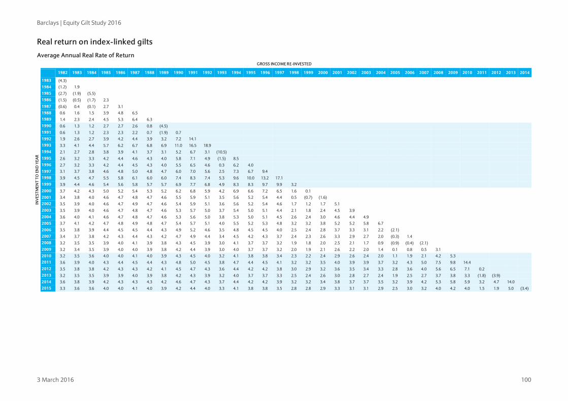
Barclays | Equity Gilt Study 2016
3 March 2016 100
Real return on index-linked gilts
Average Annual Real Rate of Return GROSS INCOME RE-INVESTED
INV
ESTM
ENT
TO E
ND
YEA
R
1982 1983 1984 1985 1986 1987 1988 1989 1990 1991 1992 1993 1994 1995 1996 1997 1998 1999 2000 2001 2002 2003 2004 2005 2006 2007 2008 2009 2010 2011 2012 2013 2014
1983 (4.3)
1984 (1.2) 1.9 1985 (2.7) (1.9) (5.5) 1986 (1.5) (0.5) (1.7) 2.3 1987 (0.6) 0.4 (0.1) 2.7 3.1 1988 0.6 1.6 1.5 3.9 4.8 6.5 1989 1.4 2.3 2.4 4.5 5.3 6.4 6.3 1990 0.6 1.3 1.2 2.7 2.7 2.6 0.8 (4.5) 1991 0.6 1.3 1.2 2.3 2.3 2.2 0.7 (1.9) 0.7 1992 1.9 2.6 2.7 3.9 4.2 4.4 3.9 3.2 7.2 14.1 1993 3.3 4.1 4.4 5.7 6.2 6.7 6.8 6.9 11.0 16.5 18.9 1994 2.1 2.7 2.8 3.8 3.9 4.1 3.7 3.1 5.2 6.7 3.1 (10.5) 1995 2.6 3.2 3.3 4.2 4.4 4.6 4.3 4.0 5.8 7.1 4.9 (1.5) 8.5 1996 2.7 3.2 3.3 4.2 4.4 4.5 4.3 4.0 5.5 6.5 4.6 0.3 6.2 4.0 1997 3.1 3.7 3.8 4.6 4.8 5.0 4.8 4.7 6.0 7.0 5.6 2.5 7.3 6.7 9.4 1998 3.9 4.5 4.7 5.5 5.8 6.1 6.0 6.0 7.4 8.3 7.4 5.3 9.6 10.0 13.2 17.1 1999 3.9 4.4 4.6 5.4 5.6 5.8 5.7 5.7 6.9 7.7 6.8 4.9 8.3 8.3 9.7 9.9 3.2 2000 3.7 4.2 4.3 5.0 5.2 5.4 5.3 5.2 6.2 6.8 5.9 4.2 6.9 6.6 7.2 6.5 1.6 0.1 2001 3.4 3.8 4.0 4.6 4.7 4.8 4.7 4.6 5.5 5.9 5.1 3.5 5.6 5.2 5.4 4.4 0.5 (0.7) (1.6) 2002 3.5 3.9 4.0 4.6 4.7 4.9 4.7 4.6 5.4 5.9 5.1 3.6 5.6 5.2 5.4 4.6 1.7 1.2 1.7 5.1 2003 3.5 3.9 4.0 4.6 4.7 4.8 4.7 4.6 5.3 5.7 5.0 3.7 5.4 5.0 5.1 4.4 2.1 1.8 2.4 4.5 3.9 2004 3.6 4.0 4.1 4.6 4.7 4.8 4.7 4.6 5.3 5.6 5.0 3.8 5.3 5.0 5.1 4.5 2.6 2.4 3.0 4.6 4.4 4.9 2005 3.7 4.1 4.2 4.7 4.8 4.9 4.8 4.7 5.4 5.7 5.1 4.0 5.5 5.2 5.3 4.8 3.2 3.2 3.8 5.2 5.2 5.8 6.7
2006 3.5 3.8 3.9 4.4 4.5 4.5 4.4 4.3 4.9 5.2 4.6 3.5 4.8 4.5 4.5 4.0 2.5 2.4 2.8 3.7 3.3 3.1 2.2 (2.1) 2007 3.4 3.7 3.8 4.2 4.3 4.4 4.3 4.2 4.7 4.9 4.4 3.4 4.5 4.2 4.3 3.7 2.4 2.3 2.6 3.3 2.9 2.7 2.0 (0.3) 1.4 2008 3.2 3.5 3.5 3.9 4.0 4.1 3.9 3.8 4.3 4.5 3.9 3.0 4.1 3.7 3.7 3.2 1.9 1.8 2.0 2.5 2.1 1.7 0.9 (0.9) (0.4) (2.1) 2009 3.2 3.4 3.5 3.9 4.0 4.0 3.9 3.8 4.2 4.4 3.9 3.0 4.0 3.7 3.7 3.2 2.0 1.9 2.1 2.6 2.2 2.0 1.4 0.1 0.8 0.5 3.1 2010 3.2 3.5 3.6 4.0 4.0 4.1 4.0 3.9 4.3 4.5 4.0 3.2 4.1 3.8 3.8 3.4 2.3 2.2 2.4 2.9 2.6 2.4 2.0 1.1 1.9 2.1 4.2 5.3 2011 3.6 3.9 4.0 4.3 4.4 4.5 4.4 4.3 4.8 5.0 4.5 3.8 4.7 4.4 4.5 4.1 3.2 3.2 3.5 4.0 3.9 3.9 3.7 3.2 4.3 5.0 7.5 9.8 14.4 2012 3.5 3.8 3.8 4.2 4.3 4.3 4.2 4.1 4.5 4.7 4.3 3.6 4.4 4.2 4.2 3.8 3.0 2.9 3.2 3.6 3.5 3.4 3.3 2.8 3.6 4.0 5.6 6.5 7.1 0.2 2013 3.2 3.5 3.5 3.9 3.9 4.0 3.9 3.8 4.2 4.3 3.9 3.2 4.0 3.7 3.7 3.3 2.5 2.4 2.6 3.0 2.8 2.7 2.4 1.9 2.5 2.7 3.7 3.8 3.3 (1.8) (3.9) 2014 3.6 3.8 3.9 4.2 4.3 4.3 4.3 4.2 4.6 4.7 4.3 3.7 4.4 4.2 4.2 3.9 3.2 3.2 3.4 3.8 3.7 3.7 3.5 3.2 3.9 4.2 5.3 5.8 5.9 3.2 4.7 14.0 2015 3.3 3.6 3.6 4.0 4.0 4.1 4.0 3.9 4.2 4.4 4.0 3.3 4.1 3.8 3.8 3.5 2.8 2.8 2.9 3.3 3.1 3.1 2.9 2.5 3.0 3.2 4.0 4.2 4.0 1.5 1.9 5.0 (3.4)

Barclays | Equity Gilt Study 2016
3 March 2016 101
Real Value of £100 Invested GROSS INCOME RE-INVESTED
INV
ESTM
ENT
TO E
ND
YEA
R
1982 1983 1984 1985 1986 1987 1988 1989 1990 1991 1992 1993 1994 1995 1996 1997 1998 1999 2000 2001 2002 2003 2004 2005 2006 2007 2008 2009 2010 2011 2012 2013 2014
1983 96
1984 98 102 1985 92 96 94 1986 94 98 97 102 1987 97 102 100 105 103 1988 103 108 106 112 110 106 1989 110 115 113 119 117 113 106 1990 105 110 108 114 111 108 102 95 1991 106 111 108 115 112 109 102 96 101 1992 121 126 124 131 128 124 117 110 115 114 1993 144 150 147 156 152 148 139 130 137 136 119 1994 128 134 132 139 136 132 124 117 122 121 106 89 1995 139 146 143 151 148 143 135 127 133 132 115 97 108 1996 145 151 148 157 154 149 140 132 138 137 120 101 113 104 1997 158 166 162 172 168 163 153 144 151 150 131 110 123 114 109 1998 186 194 190 201 197 191 179 169 177 175 154 129 144 133 128 117 1999 191 200 196 208 203 197 185 174 182 181 158 133 149 137 132 121 103 2000 192 200 196 208 203 197 185 174 182 181 159 133 149 138 132 121 103 100 2001 189 197 193 205 200 194 182 171 179 178 156 131 147 135 130 119 102 99 98 2002 198 207 203 215 210 204 191 180 189 187 164 138 154 142 137 125 107 104 103 105 2003 206 215 211 223 218 212 199 187 196 194 170 143 160 148 142 130 111 108 107 109 104 2004 216 226 221 234 229 222 209 196 206 204 179 150 168 155 149 136 116 113 113 115 109 105 2005 231 241 236 250 244 237 223 210 219 218 191 161 179 165 159 145 124 120 120 122 116 112 107 2006 226 236 231 245 239 232 218 205 215 213 187 157 176 162 156 142 122 118 118 120 114 110 105 98 2007 229 239 235 248 243 236 221 208 218 216 190 160 178 164 158 144 123 120 119 121 116 111 106 99 101 2008 224 234 230 243 238 231 217 204 213 212 186 156 175 161 155 141 121 117 117 119 113 109 104 97 99 98 2009 231 241 237 251 245 238 223 210 220 218 191 161 180 166 160 146 125 121 121 123 117 112 107 100 102 101 103 2010 243 254 249 264 258 250 235 221 232 230 202 170 190 175 168 154 131 127 127 129 123 118 113 106 108 106 109 105 2011 278 291 285 302 295 287 269 253 265 263 231 194 217 200 192 176 150 146 145 148 141 135 129 121 123 122 124 121 114 2012 279 292 286 303 296 287 270 254 266 264 231 194 217 200 193 176 150 146 146 148 141 136 129 121 124 122 124 121 115 100 2013 268 280 275 291 285 276 259 244 255 254 222 187 209 193 185 169 145 140 140 142 135 130 124 116 119 117 120 116 110 96 96 2014 306 320 314 332 324 315 296 278 291 289 253 213 238 220 211 193 165 160 160 162 154 149 142 133 136 134 136 132 126 110 110 114 2015 296 309 303 321 314 304 286 269 281 279 245 206 230 212 204 187 159 155 154 157 149 144 137 128 131 129 132 128 121 106 106 110 97

LAST PAGE
Analyst Certification We, Christian Keller, Michael Gapen, Rob Martin, Sreekala Kochugovindan, Marvin Barth, Zoso Davies, Antonio Garcia Pascual and Giuseppe Maraffino, hereby certify (1) that the views expressed in this research report accurately reflect our personal views about any or all of the subject securities or issuers referred to in this research report and (2) no part of our compensation was, is or will be directly or indirectly related to the specific recommendations or views expressed in this research report. Each research report excerpted herein was certified under SEC Regulation AC by the analyst primarily responsible for such report as follows: I hereby certify that: 1) the views expressed in this research report accurately reflect my personal views about any or all of the subject securities referred to in this report and; 2) no part of my compensation was, is or will be directly or indirectly related to the specific recommendations or views expressed in this report. Important Disclosures: Barclays Research is a part of the Investment Bank of Barclays Bank PLC and its affiliates (collectively and each individually, "Barclays"). Where any companies are the subject of this research report, for current important disclosures regarding those companies please send a written request to: Barclays Research Compliance, 745 Seventh Avenue, 13th Floor, New York, NY 10019 or refer to http://publicresearch.barclays.com or call 212-526-1072. Barclays Capital Inc. and/or one of its affiliates does and seeks to do business with companies covered in its research reports. As a result, investors should be aware that Barclays may have a conflict of interest that could affect the objectivity of this report. Barclays Capital Inc. and/or one of its affiliates regularly trades, generally deals as principal and generally provides liquidity (as market maker or otherwise) in the debt securities that are the subject of this research report (and related derivatives thereof). Barclays trading desks may have either a long and / or short position in such securities, other financial instruments and / or derivatives, which may pose a conflict with the interests of investing customers. Where permitted and subject to appropriate information barrier restrictions, Barclays fixed income research analysts regularly interact with its trading desk personnel regarding current market conditions and prices. Barclays fixed income research analysts receive compensation based on various factors including, but not limited to, the quality of their work, the overall performance of the firm (including the profitability of the Investment Banking Department), the profitability and revenues of the Markets business and the potential interest of the firm's investing clients in research with respect to the asset class covered by the analyst. To the extent that any historical pricing information was obtained from Barclays trading desks, the firm makes no representation that it is accurate or complete. All levels, prices and spreads are historical and do not represent current market levels, prices or spreads, some or all of which may have changed since the publication of this document. The Investment Bank's Research Department produces various types of research including, but not limited to, fundamental analysis, equity-linked analysis, quantitative analysis, and trade ideas. Recommendations contained in one type of research may differ from recommendations contained in other types of research, whether as a result of differing time horizons, methodologies, or otherwise. Unless otherwise indicated, trade ideas contained herein are provided as of the date of this report and are subject to change without notice due to changes in prices. In order to access Barclays Statement regarding Research Dissemination Policies and Procedures, please refer to http://publicresearch.barcap.com/static/S_ResearchDissemination.html. In order to access Barclays Research Conflict Management Policy Statement, please refer to: http://publicresearch.barcap.com/static/S_ConflictManagement.html. Barclays legal entities involved in publishing research: Barclays Bank PLC (Barclays, UK) Barclays Capital Inc. (BCI, US) Barclays Securities Japan Limited (BSJL, Japan) Barclays Bank PLC, Tokyo branch (Barclays Bank, Japan) Barclays Bank PLC, Hong Kong branch (Barclays Bank, Hong Kong) Barclays Capital Canada Inc. (BCCI, Canada) Absa Bank Limited (Absa, South Africa) Barclays Bank Mexico, S.A. (BBMX, Mexico) Barclays Capital Securities Taiwan Limited (BCSTW, Taiwan) Barclays Capital Securities Limited (BCSL, South Korea) Barclays Securities (India) Private Limited (BSIPL, India) Barclays Bank PLC, India branch (Barclays Bank, India) Barclays Bank PLC, Singapore branch (Barclays Bank, Singapore) Barclays Bank PLC, Australia branch (Barclays Bank, Australia)
Disclaimer: This publication has been produced by the Investment Bank of Barclays Bank PLC and/or one or more of its affiliates (collectively and each individually, "Barclays"). It has been distributed by one or more Barclays legal entities that are a part of the Investment Bank as provided below. It is provided to our clients for information purposes only, and Barclays makes no express or implied warranties, and expressly disclaims all warranties of merchantability or fitness for a particular purpose or use with respect to any data included in this publication. Barclays will not treat unauthorized recipients of this report as its clients and accepts no liability for use by them of the contents which may not be suitable for their personal use. Prices shown are indicative and Barclays is not offering to buy or sell or soliciting offers to buy or sell any financial instrument. Without limiting any of the foregoing and to the extent permitted by law, in no event shall Barclays, nor any affiliate, nor any of their respective officers, directors, partners, or employees have any liability for (a) any special, punitive, indirect, or consequential damages; or (b) any lost profits, lost revenue, loss of anticipated savings or loss of opportunity or other financial loss, even if notified of the possibility of such damages, arising from any use of this publication or its contents. Other than disclosures relating to Barclays, the information contained in this publication has been obtained from sources that Barclays Research believes to be reliable, but Barclays does not represent or warrant that it is accurate or complete. Barclays is not responsible for, and makes no warranties whatsoever as to, the content of any third-party web site accessed via a hyperlink in this publication and such information is not incorporated by reference. The views in this publication are those of the author(s) and are subject to change, and Barclays has no obligation to update its opinions or the information in this publication. If this publication contains recommendations, those recommendations reflect solely and exclusively those of the authoring analyst(s), and such opinions were prepared independently of any other interests, including those of Barclays and/or its affiliates. This publication does not constitute personal investment advice or take into account the individual financial circumstances or objectives of the clients who receive it. The securities discussed herein may not be suitable for all investors. Barclays recommends that investors independently evaluate each issuer, security or instrument discussed herein and consult any independent advisors they believe necessary. The value of and income from any investment may fluctuate from day to

LAST PAGE
day as a result of changes in relevant economic markets (including changes in market liquidity). The information herein is not intended to predict actual results, which may differ substantially from those reflected. Past performance is not necessarily indicative of future results. This document is being distributed (1) only by or with the approval of an authorised person (Barclays Bank PLC) or (2) to, and is directed at (a) persons in the United Kingdom having professional experience in matters relating to investments and who fall within the definition of "investment professionals" in Article 19(5) of the Financial Services and Markets Act 2000 (Financial Promotion) Order 2005 (the "Order"); or (b) high net worth companies, unincorporated associations and partnerships and trustees of high value trusts as described in Article 49(2) of the Order; or (c) other persons to whom it may otherwise lawfully be communicated (all such persons being "Relevant Persons"). Any investment or investment activity to which this communication relates is only available to and will only be engaged in with Relevant Persons. Any other persons who receive this communication should not rely on or act upon it. Barclays Bank PLC is authorised by the Prudential Regulation Authority and regulated by the Financial Conduct Authority and the Prudential Regulation Authority and is a member of the London Stock Exchange. The Investment Bank of Barclays Bank PLC undertakes U.S. securities business in the name of its wholly owned subsidiary Barclays Capital Inc., a FINRA and SIPC member. Barclays Capital Inc., a U.S. registered broker/dealer, is distributing this material in the United States and, in connection therewith accepts responsibility for its contents. Any U.S. person wishing to effect a transaction in any security discussed herein should do so only by contacting a representative of Barclays Capital Inc. in the U.S. at 745 Seventh Avenue, New York, New York 10019. Non-U.S. persons should contact and execute transactions through a Barclays Bank PLC branch or affiliate in their home jurisdiction unless local regulations permit otherwise. Barclays Bank PLC, Paris Branch (registered in France under Paris RCS number 381 066 281) is regulated by the Autorité des marchés financiers and the Autorité de contrôle prudentiel. Registered office 34/36 Avenue de Friedland 75008 Paris. This material is distributed in Canada by Barclays Capital Canada Inc., a registered investment dealer, a Dealer Member of IIROC (www.iiroc.ca), and a Member of the Canadian Investor Protection Fund (CIPF). Subject to the conditions of this publication as set out above, the Corporate & Investment Banking Division of Absa Bank Limited, an authorised financial services provider (Registration No.: 1986/004794/06. Registered Credit Provider Reg No NCRCP7), is distributing this material in South Africa. Absa Bank Limited is regulated by the South African Reserve Bank. This publication is not, nor is it intended to be, advice as defined and/or contemplated in the (South African) Financial Advisory and Intermediary Services Act, 37 of 2002, or any other financial, investment, trading, tax, legal, accounting, retirement, actuarial or other professional advice or service whatsoever. Any South African person or entity wishing to effect a transaction in any security discussed herein should do so only by contacting a representative of the Corporate & Investment Banking Division of Absa Bank Limited in South Africa, 15 Alice Lane, Sandton, Johannesburg, Gauteng 2196. Absa Bank Limited is a member of the Barclays group. In Japan, foreign exchange research reports are prepared and distributed by Barclays Bank PLC Tokyo Branch. Other research reports are distributed to institutional investors in Japan by Barclays Securities Japan Limited. Barclays Securities Japan Limited is a joint-stock company incorporated in Japan with registered office of 6-10-1 Roppongi, Minato-ku, Tokyo 106-6131, Japan. It is a subsidiary of Barclays Bank PLC and a registered financial instruments firm regulated by the Financial Services Agency of Japan. Registered Number: Kanto Zaimukyokucho (kinsho) No. 143. Barclays Bank PLC, Hong Kong Branch is distributing this material in Hong Kong as an authorised institution regulated by the Hong Kong Monetary Authority. Registered Office: 41/F, Cheung Kong Center, 2 Queen's Road Central, Hong Kong. Information on securities/instruments that trade in Taiwan or written by a Taiwan-based research analyst is distributed by Barclays Capital Securities Taiwan Limited to its clients. The material on securities/instruments not traded in Taiwan is not to be construed as 'recommendation' in Taiwan. Barclays Capital Securities Taiwan Limited does not accept orders from clients to trade in such securities. This material may not be distributed to the public media or used by the public media without prior written consent of Barclays. This material is distributed in South Korea by Barclays Capital Securities Limited, Seoul Branch. All Indian securities-related research and other equity research produced by the Investment Bank are distributed in India by Barclays Securities (India) Private Limited (BSIPL). BSIPL is a company incorporated under the Companies Act, 1956 having CIN U67120MH2006PTC161063. BSIPL is registered and regulated by the Securities and Exchange Board of India (SEBI) as a Research Analyst: INH000001519; Portfolio Manager INP000002585; Stock Broker/Trading and Clearing Member: National Stock Exchange of India Limited (NSE) Capital Market INB231292732, NSE Futures & Options INF231292732, NSE Currency derivatives INE231450334, Bombay Stock Exchange Limited (BSE) Capital Market INB011292738, BSE Futures & Options INF011292738; Merchant Banker: INM000011195; Depository Participant (DP) with the National Securities & Depositories Limited (NSDL): DP ID: IN-DP-NSDL-299-2008; Investment Adviser: INA000000391. The registered office of BSIPL is at 208, Ceejay House, Shivsagar Estate, Dr. A. Besant Road, Worli, Mumbai – 400 018, India. Telephone No: +91 2267196000. Fax number: +91 22 67196100. Any other reports produced by the Investment Bank are distributed in India by Barclays Bank PLC, India Branch, an associate of BSIPL in India that is registered with Reserve Bank of India (RBI) as a Banking Company under the provisions of The Banking Regulation Act, 1949 (Regn No BOM43) and registered with SEBI as Merchant Banker (Regn No INM000002129) and also as Banker to the Issue (Regn No INBI00000950). Barclays Investments and Loans (India) Limited, registered with RBI as Non Banking Financial Company (Regn No RBI CoR-07-00258), and Barclays Wealth Trustees (India) Private Limited, registered with Registrar of Companies (CIN U93000MH2008PTC188438), are associates of BSIPL in India that are not authorised to distribute any reports produced by the Investment Bank. Barclays Bank PLC Frankfurt Branch distributes this material in Germany under the supervision of Bundesanstalt für Finanzdienstleistungsaufsicht (BaFin). This material is distributed in Malaysia by Barclays Capital Markets Malaysia Sdn Bhd. This material is distributed in Brazil by Banco Barclays S.A. This material is distributed in Mexico by Barclays Bank Mexico, S.A. Barclays Bank PLC in the Dubai International Financial Centre (Registered No. 0060) is regulated by the Dubai Financial Services Authority (DFSA). Principal place of business in the Dubai International Financial Centre: The Gate Village, Building 4, Level 4, PO Box 506504, Dubai, United Arab Emirates. Barclays Bank PLC-DIFC Branch, may only undertake the financial services activities that fall within the scope of its existing DFSA licence. Related financial products or services are only available to Professional Clients, as defined by the Dubai Financial Services Authority. Barclays Bank PLC in the UAE is regulated by the Central Bank of the UAE and is licensed to conduct business activities as a branch of a commercial bank incorporated outside the UAE in Dubai (Licence No.: 13/1844/2008, Registered Office: Building No. 6, Burj Dubai Business Hub, Sheikh Zayed Road, Dubai City) and Abu Dhabi (Licence No.: 13/952/2008, Registered Office: Al Jazira Towers, Hamdan Street, PO Box 2734, Abu Dhabi). Barclays Bank PLC in the Qatar Financial Centre (Registered No. 00018) is authorised by the Qatar Financial Centre Regulatory Authority (QFCRA). Barclays Bank PLC-QFC Branch may only undertake the regulated activities that fall within the scope of its existing QFCRA licence. Principal place of business in Qatar: Qatar Financial Centre, Office 1002, 10th Floor, QFC Tower, Diplomatic Area, West Bay, PO Box 15891, Doha, Qatar. Related financial products or services are only available to Business Customers as defined by the Qatar Financial Centre Regulatory Authority. This material is distributed in the UAE (including the Dubai International Financial Centre) and Qatar by Barclays Bank PLC. This material is not intended for investors who are not Qualified Investors according to the laws of the Russian Federation as it might contain information about or description of the features of financial instruments not admitted for public offering and/or circulation in the Russian Federation and thus not eligible for non-Qualified Investors. If you are not a Qualified Investor according to the laws of the Russian Federation, please dispose of any copy of this material in your possession. This material is distributed in Singapore by the Singapore branch of Barclays Bank PLC, a bank licensed in Singapore by the Monetary Authority of Singapore. For matters in connection with this report, recipients in Singapore may contact the Singapore branch of Barclays Bank PLC, whose registered address is 10 Marina Boulevard, #23-01 Marina Bay Financial Centre Tower 2, Singapore 018983.

LAST PAGE
Barclays Bank PLC, Australia Branch (ARBN 062 449 585, AFSL 246617) is distributing this material in Australia. It is directed at 'wholesale clients' as defined by Australian Corporations Act 2001. IRS Circular 230 Prepared Materials Disclaimer: Barclays does not provide tax advice and nothing contained herein should be construed to be tax advice. Please be advised that any discussion of U.S. tax matters contained herein (including any attachments) (i) is not intended or written to be used, and cannot be used, by you for the purpose of avoiding U.S. tax-related penalties; and (ii) was written to support the promotion or marketing of the transactions or other matters addressed herein. Accordingly, you should seek advice based on your particular circumstances from an independent tax advisor. © Copyright Barclays Bank PLC (2016). All rights reserved. No part of this publication may be reproduced or redistributed in any manner without the prior written permission of Barclays. Barclays Bank PLC is registered in England No. 1026167. Registered office 1 Churchill Place, London, E14 5HP. Additional information regarding this publication will be furnished upon request.


