3. The Gaussian kernel Of all things, man is the measure. Protagoras the Sophist (480-411 B.C.) 3.1 The Gaussian kernel The Gaussian (better Gaußian) kernel is named after Carl Friedrich Gauß (1777-1855), a brilliant German mathematician. This chapter discusses many of the attractive and special properties of the Gaussian kernel. << FrontEndVision`FEV`; Show@Import@"Gauss10DM.gif"D, ImageSize -> 280D; Figure 3.1 The Gaussian kernel is apparent on every German banknote of DM 10,- where it is depicted next to its famous inventor when he was 55 years old. The new Euro replaces these banknotes. See also: http://scienceworld.wolfram.com/biography/Gauss.html. The Gaussian kernel is defined in 1-D, 2D and N-D respectively as G 1 D H x; sL = 1 è!!!!!!! 2 p s e - x 2 2 s 2 , G 2 D H x, y; sL = 1 2 ps 2 e - x 2 +y 2 2 s 2 , G ND H x ” ; sL = 1 I è!!!!!!! 2 p sM N e - » x ” ÷ » 2 2 s 2 The s determines the width of the Gaussian kernel. In statistics, when we consider the Gaussian probability density function it is called the standard deviation, and the square of it, s 2 , the variance. In the rest of this book, when we consider the Gaussian as an aperture function of some observation, we will refer to s as the inner scale or shortly scale. In the whole of this book the scale can only take positive values, s> 0 . In the process of observation s can never become zero. For, this would imply making an observation through an infinitesimally small aperture, which is impossible. The factor of 2 in the exponent is a matter of convention, because we then have a 'cleaner' formula for the diffusion equation, as we will see later on. The semicolon between the spatial and scale parameters is conventionally put there to make the difference between these parameters explicit. 3. The Gaussian kernel 37
Transcript
3. The Gaussian kernelOf all things, man is the measure.
Protagoras the Sophist (480-411 B.C.)
3.1 The Gaussian kernel
The Gaussian (better Gaußian) kernel is named after Carl Friedrich Gauß (1777-1855), abrilliant German mathematician. This chapter discusses many of the attractive and specialproperties of the Gaussian kernel.
Figure 3.1 The Gaussian kernel is apparent on every German banknote of DM 10,- where itis depicted next to its famous inventor when he was 55 years old. The new Euro replacesthese banknotes. See also: http://scienceworld.wolfram.com/biography/Gauss.html.
The Gaussian kernel is defined in 1-D, 2D and N-D respectively as
The s determines the width of the Gaussian kernel. In statistics, when we consider theGaussian probability density function it is called the standard deviation, and the square of it,s2 , the variance. In the rest of this book, when we consider the Gaussian as an aperturefunction of some observation, we will refer to s as the inner scale or shortly scale.
In the whole of this book the scale can only take positive values, s > 0 . In the process ofobservation s can never become zero. For, this would imply making an observation throughan infinitesimally small aperture, which is impossible. The factor of 2 in the exponent is amatter of convention, because we then have a 'cleaner' formula for the diffusion equation, aswe will see later on. The semicolon between the spatial and scale parameters isconventionally put there to make the difference between these parameters explicit.
3. The Gaussian kernel 37
The scale-dimension is not just another spatial dimension, as we will thoroughly discuss inthe remainder of this book.
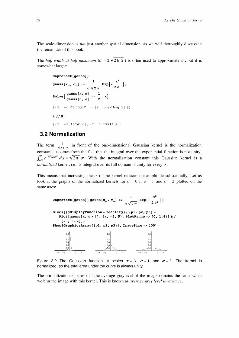
The half width at half maximum (s = 2 è!!!!!!!!!!!2 ln 2 ) is often used to approximate s , but it is
in front of the one-dimensional Gaussian kernel is the normalizationconstant. It comes from the fact that the integral over the exponential function is not unity:Ÿ-¶
¶e-x2 ê2 s2
„ x =è!!!!!!!!
2 p s . With the normalization constant this Gaussian kernel is anormalized kernel, i.e. its integral over its full domain is unity for every s.
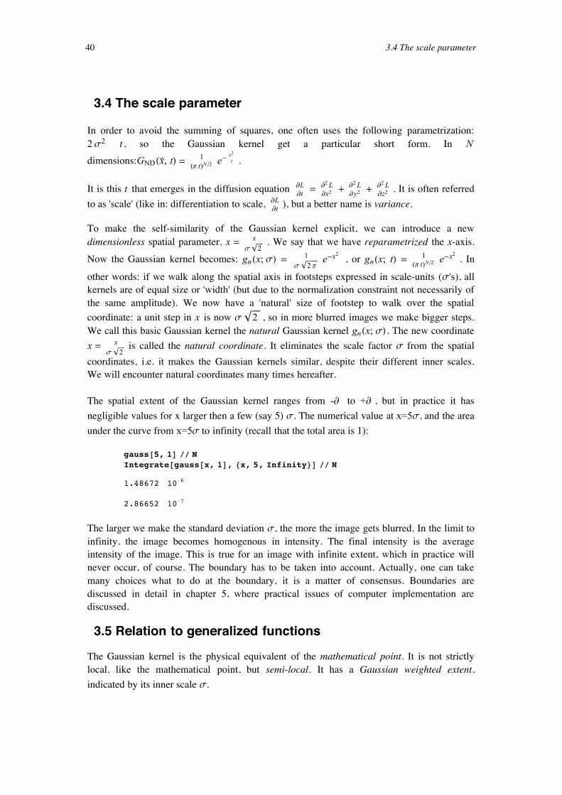
This means that increasing the s of the kernel reduces the amplitude substantially. Let uslook at the graphs of the normalized kernels for s = 0.3 , s = 1 and s = 2 plotted on thesame axes:
Figure 3.2 The Gaussian function at scales s = .3 , s = 1 and s = 2 . The kernel isnormalized, so the total area under the curve is always unity.
The normalization ensures that the average graylevel of the image remains the same whenwe blur the image with this kernel. This is known as average grey level invariance.
38 3.1 The Gaussian kernel
3.3 Cascade property, selfsimilarity
The shape of the kernel remains the same, irrespective of the s. When we convolve twoGaussian kernels we get a new wider Gaussian with a variance s2 which is the sum of thevariances of the constituting Gaussians: gnew Hx”; s1
This phenomenon, i.e. that a new function emerges that is similar to the constitutingfunctions, is called self-similarity.
The Gaussian is a self-similar function. Convolution with a Gaussian is a linear operation, soa convolution with a Gaussian kernel followed by a convolution with again a Gaussiankernel is equivalent to convolution with the broader kernel. Note that the squares of s add,not the s's themselves. Of course we can concatenate as many blurring steps as we want tocreate a larger blurring step. With analogy to a cascade of waterfalls spanning the sameheight as the total waterfall, this phenomenon is also known as the cascade smoothingproperty.Famous examples of self-similar functions are fractals. This shows the famous Mandelbrotfractal:
Figure 3.3 The Mandelbrot fractal is a famous example of a self-similar function. Source:www.mathforum.org. See also mathworld.wolfram.com/MandelbrotSet.html.
3. The Gaussian kernel 39
3.4 The scale parameter
In order to avoid the summing of squares, one often uses the following parametrization:2 s2 Ø t , so the Gaussian kernel get a particular short form. In Ndimensions:GND Hx”, tL = 1ÅÅÅÅÅÅÅÅÅÅÅÅÅÅÅÅÅHp tLN ê2 e- x2
ÅÅÅÅÅÅÅÅt .
It is this t that emerges in the diffusion equation ∑LÅÅÅÅÅÅÅ∑t = ∑2 LÅÅÅÅÅÅÅÅÅÅ∑x2 + ∑2 LÅÅÅÅÅÅÅÅÅÅ∑y2 + ∑2 LÅÅÅÅÅÅÅÅÅÅ∑z2 . It is often referredto as 'scale' (like in: differentiation to scale, ∑LÅÅÅÅÅÅÅ∑t ), but a better name is variance.
To make the self-similarity of the Gaussian kernel explicit, we can introduce a newdimensionless spatial parameter, xè = xÅÅÅÅÅÅÅÅÅÅÅÅÅÅ
s è!!!!
2. We say that we have reparametrized the x-axis.
Now the Gaussian kernel becomes: gn Hxè; sL = 1ÅÅÅÅÅÅÅÅÅÅÅÅÅÅÅÅÅÅs
è!!!!!!!2 p
e-xè2 , or gn Hxè ; tL = 1ÅÅÅÅÅÅÅÅÅÅÅÅÅÅÅÅÅHp tLNê2 e-xè2 . In
other words: if we walk along the spatial axis in footsteps expressed in scale-units (s's), allkernels are of equal size or 'width' (but due to the normalization constraint not necessarily ofthe same amplitude). We now have a 'natural' size of footstep to walk over the spatialcoordinate: a unit step in x is now s è!!!!
2 , so in more blurred images we make bigger steps.We call this basic Gaussian kernel the natural Gaussian kernel gn Hxè; sL . The new coordinatexè = xÅÅÅÅÅÅÅÅÅÅÅÅÅÅ
s è!!!!
2is called the natural coordinate. It eliminates the scale factor s from the spatial
coordinates, i.e. it makes the Gaussian kernels similar, despite their different inner scales.We will encounter natural coordinates many times hereafter.
The spatial extent of the Gaussian kernel ranges from -¶ to +¶, but in practice it hasnegligible values for x larger then a few (say 5) s. The numerical value at x=5s, and the areaunder the curve from x=5s to infinity (recall that the total area is 1):
gauss@5, 1D êê NIntegrate@gauss@x, 1D, 8x, 5, Infinity<D êê N
1.48672µ 10-6
2.86652µ 10-7
The larger we make the standard deviation s, the more the image gets blurred. In the limit toinfinity, the image becomes homogenous in intensity. The final intensity is the averageintensity of the image. This is true for an image with infinite extent, which in practice willnever occur, of course. The boundary has to be taken into account. Actually, one can takemany choices what to do at the boundary, it is a matter of consensus. Boundaries arediscussed in detail in chapter 5, where practical issues of computer implementation arediscussed.
3.5 Relation to generalized functions
The Gaussian kernel is the physical equivalent of the mathematical point. It is not strictlylocal, like the mathematical point, but semi-local. It has a Gaussian weighted extent,indicated by its inner scale s.
Because scale-space theory is revolving around the Gaussian function and its derivatives as aphysical differential operator (in more detail explained in the next chapter), we will focushere on some mathematical notions that are directly related, i.e. the mathematical notionsunderlying sampling of values from functions and their derivatives at selected points (i.e. thatis why it is referred to as sampling). The mathematical functions involved are thegeneralized functions, i.e. the Delta-Dirac function, the Heaviside function and the errorfunction. In the next section we study these functions in detail.
40 3.4 The scale parameter
Because scale-space theory is revolving around the Gaussian function and its derivatives as aphysical differential operator (in more detail explained in the next chapter), we will focushere on some mathematical notions that are directly related, i.e. the mathematical notionsunderlying sampling of values from functions and their derivatives at selected points (i.e. thatis why it is referred to as sampling). The mathematical functions involved are thegeneralized functions, i.e. the Delta-Dirac function, the Heaviside function and the errorfunction. In the next section we study these functions in detail.
When we take the limit as the inner scale goes down to zero (remember that s can only takepositive values for a physically realistic system), we get the mathematical delta function, orDirac delta function, d(x). This function is everywhere zero except in x = 0, where it hasinfinite amplitude and zero width, its area is unity.
lims∞0 J 1ÅÅÅÅÅÅÅÅÅÅÅÅÅÅÅÅÅÅè!!!!!!!2 p s
e- x2ÅÅÅÅÅÅÅÅÅÅÅÅÅ2 s2 N = dHxL.
d(x) is called the sampling function in mathematics, because the Dirac delta functionadequately samples just one point out of a function when integrated. It is assumed that f HxLis continuous at x = a:
‡-¶
¶
DiracDelta@x - aD f@xD „x
f@aDThe sampling property of derivatives of the Dirac delta function is shown below:
‡-¶
¶
D@DiracDelta@xD, 8x, 2<D f@xD „x
f££ @0DThe delta function was originally proposed by the eccentric Victorian mathematician OliverHeaviside (1880-1925, see also [Pickover1998]). Story goes that mathematicians called thisfunction a "monstrosity", but it did work! Around 1950 physicist Paul Dirac (1902-1984)gave it new light. Mathematician Laurent Schwartz (1915-) proved it in 1951 with hisfamous "theory of distributions" (we discuss this theory in chapter 8). And today it's called"the Dirac delta function".
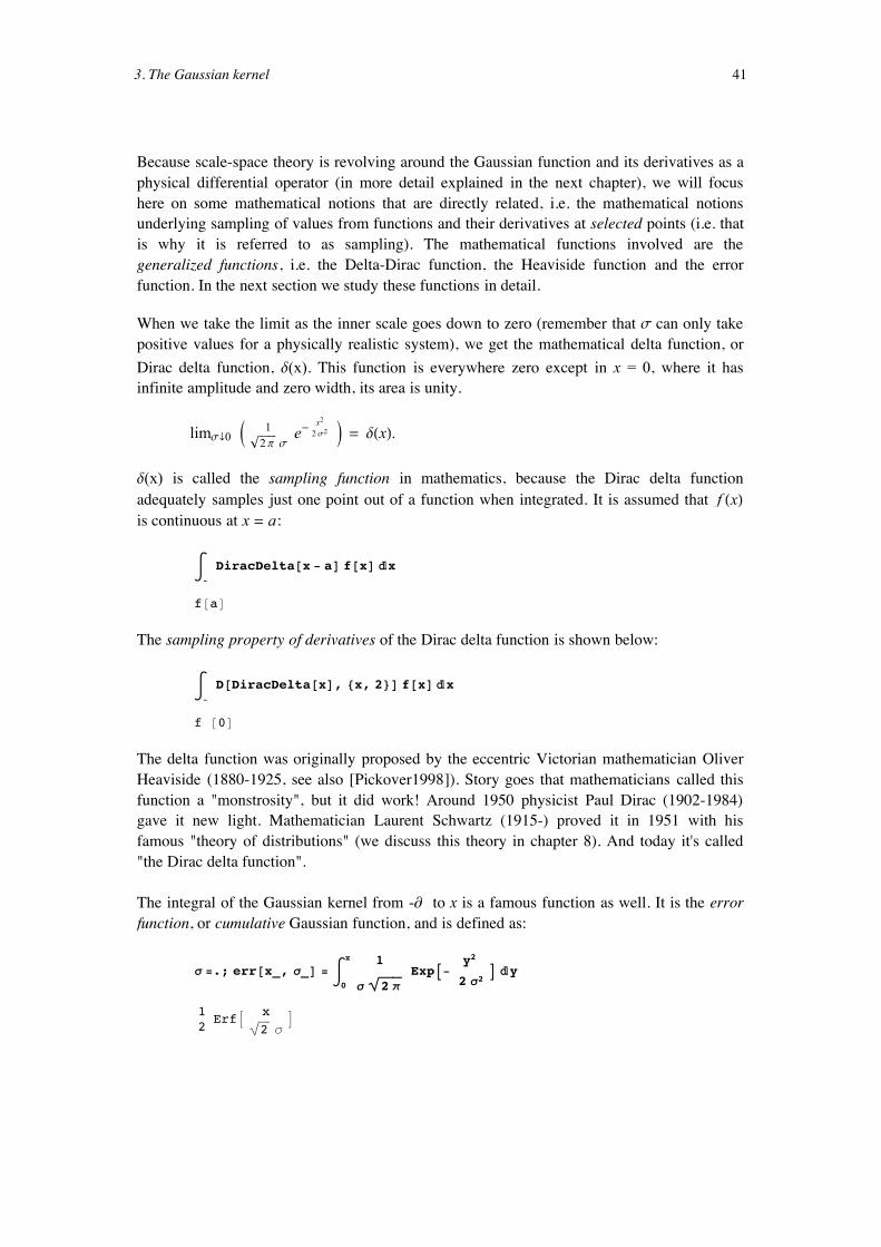
The integral of the Gaussian kernel from -¶ to x is a famous function as well. It is the errorfunction, or cumulative Gaussian function, and is defined as:
s =.; err@x_, s_D = ‡0
x 1ÅÅÅÅÅÅÅÅÅÅÅÅÅÅÅÅÅÅs
è!!!!!!!2 p
ExpA-y2
ÅÅÅÅÅÅÅÅÅÅÅÅ2 s2
E „y
1ÅÅÅÅ2 ErfA x
ÅÅÅÅÅÅÅÅÅÅÅÅÅè!!!2 sE
3. The Gaussian kernel 41
The y in the integral above is just a dummy integration variable, and is integrated out. TheMathematica error function is Erf[x].
In our integral of the Gaussian function we need to do the reparametrization x Ø xÅÅÅÅÅÅÅÅÅÅÅÅÅÅs
è!!!!2
.Again we recognize the natural coordinates. The factor 1ÅÅÅÅ2 is due to the fact that integrationstarts halfway, in x = 0.
Figure 3.4 The error function Erf[x] is the cumulative Gaussian function.
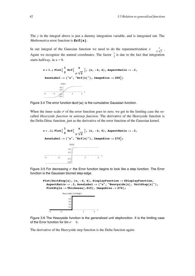
When the inner scale s of the error function goes to zero, we get in the limiting case the so-called Heavyside function or unitstep function. The derivative of the Heavyside function isthe Delta-Dirac function, just as the derivative of the error function of the Gaussian kernel.
Figure 3.6 The Heavyside function is the generalized unit stepfunction. It is the limiting caseof the Error function for lim s Ø 0 .
The derivative of the Heavyside step function is the Delta function again:
42 3.5 Relation to generalized functions
D@UnitStep@xD, xDDiracDelta@xD
3.6 Separability
The Gaussian kernel for dimensions higher than one, say N, can be described as a regularproduct of N one-dimensional kernels. Example: g2 DHx, y; s1
2 + s22L = g1 D Hx; s1
2 Lg1 D Hy; s2
2 L where the space in between is the product operator. The regular product alsoexplains the exponent N in the normalization constant for N-dimensional Gaussian kernels in(0). Because higher dimensional Gaussian kernels are regular products of one-dimensionalGaussians, they are called separable. We will use quite often this property of separability.
DisplayTogetherArray@8Plot@gauss@x, s = 1D, 8x, -3, 3<D,Plot3D@gauss@x, s = 1D gauss@y, s = 1D, 8x, -3, 3<, 8y, -3, 3<D<,ImageSize -> 440D;
-3 -2 -1 1 2 3
0.1
0.2
0.3
0.4
Figure 3.7 A product of Gaussian functions gives a higher dimensional Gaussian function.This is a consequence of the separability.
An important application is the speed improvement when implementing numerical separableconvolution. In chapter 5 we explain in detail how the convolution with a 2D (or better: N-dimensional) Gaussian kernel can be replaced by a cascade of 1D convolutions, making theprocess much more efficient because convolution with the 1D kernels requires far fewermultiplications.
3.7 Relation to binomial coefficients
Another place where the Gaussian function emerges is in expansions of powers ofpolynomials. Here is an example:
Figure 3.9 Binomial coefficients approximate a Gaussian distribution for increasing order.Here in 2 dimensions we see separability again.
3.8 The Fourier transform of the Gaussian kernel
We will regularly do our calculations in the Fourier domain, as this often turns out to beanalytically convenient or computationally efficient. The basis functions of the Fouriertransform ! are the sinusoidal functions eiwx . The definitions for the Fourier transform andits inverse are:
the Fourier transform: FHwL = ! 8 f HxL< = 1ÅÅÅÅÅÅÅÅÅÅÅÅÅÅè!!!!!!!2 p
Ÿ-¶
¶f HxL ei w x „ x
the inverse Fourier transform: ! -1 8FHwL< = 1ÅÅÅÅÅÅÅÅÅÅÅÅÅÅè!!!!!!!2 p
Ÿ-¶
¶FHwL e-i w x „ w
s =.; !gauss@w_, s_D =
SimplifyA 1ÅÅÅÅÅÅÅÅÅÅÅÅÅÅè!!!!!!!2 p
IntegrateA 1ÅÅÅÅÅÅÅÅÅÅÅÅÅÅÅÅÅÅs
è!!!!!!!2 p
ExpA-x2
ÅÅÅÅÅÅÅÅÅÅÅ2 s2
E Exp@I w xD, 8x, -¶, ¶<E,8s > 0, Im@sD == 0<E‰- 1ÅÅÅÅ2 s2 w2
ÅÅÅÅÅÅÅÅÅÅÅÅÅÅÅÅÅÅÅÅè!!!!!!!2 p
44 3.7 Relation to binomial coefficients
The Fourier transform is a standard Mathematica command:
Simplify@FourierTransform@gauss@x, sD, x, wD, s > 0D‰- 1ÅÅÅÅ2 s2 w2
ÅÅÅÅÅÅÅÅÅÅÅÅÅÅÅÅÅÅÅÅè!!!!!!!2 p
Note that different communities (mathematicians, computer scientists, engineers) havedifferent definitions for the Fourier transform. From the Mathematica help function:
With the setting FourierParametersØ{a,b} the discrete Fourier transform computedby FourierTransform is "##############»b»ÅÅÅÅÅÅÅÅÅÅÅÅÅÅÅÅÅÅH2 pL1-a Ÿ-¶
¶ f HtL ei b w t „ t . Some common choices for {a,b}are {0,1} (default), {-1,1} (data analysis), {1,-1} (signal processing).
In this book we consistently use the default definition.
So the Fourier transform of the Gaussian function is again a Gaussian function, but now ofthe frequency w. The Gaussian function is the only function with this property. Note that thescale s now appears as a multiplication with the frequency. We recognize a well-known fact:a smaller kernel in the spatial domain gives a wider kernel in the Fourier domain, and viceversa. Here we plot 3 Gaussian kernels with their Fourier transform beneath each plot:
Figure 3.10 Top row: Gaussian function at scales s=1, s=2 and s=3. Bottom row: Fouriertransform of the Gaussian function above it. Note that for wider Gaussian its Fouriertransform gets narrower and vice versa, a well known phenomenon with the Fouriertransform. Also note by checking the amplitudes that the kernel is normalized in the spatialdomain only.
There are many names for the Fourier transform ! gHw; sL of gHx; sL : when the kernelgHx; sL is considered to be the point spread function, ! gHw; sL is referred to as themodulation transfer function. When the kernel g(x;s) is considered to be a signal, ! gHw; sLis referred to as the spectrum. When applied to a signal, it operates as a lowpass filter. Let usplot the spectra of a series of such filters (with a logarithmic increase in scale) on doublelogarithmic paper:
3. The Gaussian kernel 45
There are many names for the Fourier transform ! gHw; sL of gHx; sL : when the kernelgHx; sL is considered to be the point spread function, ! gHw; sL is referred to as themodulation transfer function. When the kernel g(x;s) is considered to be a signal, ! gHw; sLis referred to as the spectrum. When applied to a signal, it operates as a lowpass filter. Let usplot the spectra of a series of such filters (with a logarithmic increase in scale) on doublelogarithmic paper:
Figure 3.11 Fourier spectra of the Gaussian kernel for an exponential range of scales s = 1
(most right graph) to s = 14.39 (most left graph). The frequency w is on a logarithmic scale.The Gaussian kernels are seen to act as low-pass filters.
Due to this behaviour the role of receptive fields as lowpass filters has long persisted. But theretina does not measure a Fourier transform of the incoming image, as we will discuss in thechapters on the visual system (chapters 9-12).
3.9 Central limit theorem
We see in the paragraph above the relation with the central limit theorem: any repetitiveoperator goes in the limit to a Gaussian function. Later, when we study the discreteimplementation of the Gaussian kernel and discrete sampled data, we will see the relationbetween interpolation schemes and the binomial coefficients. We study a repeatedconvolution of two blockfunctions with each other:
Figure 3.14 Two times a convolution of a blockfunction with the same blockfunction gives afunction that rapidly begins to look like a Gaussian function. A Gaussian kernel with s = 0.5is drawn (dotted) for comparison.
The real Gaussian is reached when we apply an infinite number of these convolutions withthe same function. It is remarkable that this result applies for the infinite repetition of anyconvolution kernel. This is the central limit theorem.
Ú Task 3.1 Show the central limit theorem in practice for a number of otherarbitrary kernels.
Figure 3.15 The slope of an isotropic Gaussian function is indicated by arrows here. There arecircularly symmetric, i.e. in all directions the same, from which the name isotropic derives.The arrows are in the direction of the normal of the intensity landscape, and are calledgradient vectors.
The Gaussian kernel as specified above is isotropic, which means that the behaviour of thefunction is in any direction the same. For 2D this means the Gaussian function is circular, for3D it looks like a fuzzy sphere.
It is of no use to speak of isotropy in 1-D. When the standard deviations in the differentdimensions are not equal, we call the Gaussian function anisotropic. An example is thepointspreadfunction of an astigmatic eye, where differences in curvature of the cornea/lens indifferent directions occur. This show an anisotropic Gaussian with anisotropy ratio of 2Hsx ê sy = 2L :
Figure 3.16 An anisotropic Gaussian kernel with anisotropy ratio sx ê sy = 2 in threeappearances. Left: DensityPlot, middle: Plot3D, right: ContourPlot.
3.11 The diffusion equation
The Gaussian function is the solution of several differential equations. It is the solution ofd yÅÅÅÅÅÅÅÅd x = yHm-xLÅÅÅÅÅÅÅÅÅÅÅÅÅÅÅÅs2 , because d yÅÅÅÅÅÅÅÅy = Hm-xLÅÅÅÅÅÅÅÅÅÅÅÅÅÅs2 d x , from which we find by integration lnI yÅÅÅÅÅÅÅy0
M = - Hm-xL2
ÅÅÅÅÅÅÅÅÅÅÅÅÅÅÅÅ2 s2
and thus y = y0 e- Hx-mL2ÅÅÅÅÅÅÅÅÅÅÅÅÅÅÅÅÅÅ
2 s2 .
It is the solution of the linear diffusion equation, ∑LÅÅÅÅÅÅÅ∑t = ∑2 LÅÅÅÅÅÅÅÅÅÅ∑x2 + ∑2 LÅÅÅÅÅÅÅÅÅÅ∑y2 = D L .
This is a partial differential equation, stating that the first derivative of the (luminance)function LHx, yL to the parameter t (time, or variance) is equal to the sum of the second orderspatial derivatives. The right hand side is also known as the Laplacian (indicated by D forany dimension, we call D the Laplacian operator), or the trace of the Hessian matrix ofsecond order derivatives:
The diffusion equation ∑uÅÅÅÅÅÅÅ∑t = D u is one of some of the most famous differential equations inphysics. It is often referred to as the heat equation. It belongs in the row of other famousequations like the Laplace equation D u = 0 , the wave equation ∑2 uÅÅÅÅÅÅÅÅÅ∑t2 = D u and theSchrödinger equation ∑uÅÅÅÅÅÅÅ∑t = i D u .
3. The Gaussian kernel 49
The diffusion equation ∑uÅÅÅÅÅÅÅ∑t = D u is one of some of the most famous differential equations inphysics. It is often referred to as the heat equation. It belongs in the row of other famousequations like the Laplace equation D u = 0 , the wave equation ∑2 uÅÅÅÅÅÅÅÅÅ∑t2 = D u and theSchrödinger equation ∑uÅÅÅÅÅÅÅ∑t = i D u .
The diffusion equation ∑uÅÅÅÅÅÅÅ∑t = D u is a linear equation. It consists of just linearly combinedderivative terms, no nonlinear exponents or functions of derivatives.
The diffused entity is the intensity in the images. The role of time is taken by the variancet = 2 s2 . The intensity is diffused over time (in our case over scale) in all directions in thesame way (this is called isotropic). E.g. in 3D one can think of the example of the intensityof an inkdrop in water, diffusing in all directions.
The diffusion equation can be derived from physical principles: the luminance can beconsidered a flow, that is pushed away from a certain location by a force equal to thegradient. The divergence of this gradient gives how much the total entity (luminance in ourcase) diminishes with time.
<< Calculus`VectorAnalysis`SetCoordinates@Cartesian@x, y, zDD;Div@ Grad@L@x, y, zDDDLH0,0,2L @x, y, zD + LH0,2,0L @x, y, zD + LH2,0,0L @x, y, zD
A very important feature of the diffusion process is that it satisfies a maximum principle[Hummel1987b]: the amplitude of local maxima are always decreasing when we go tocoarser scale, and vice versa, the amplitude of local minima always increase for coarserscale. This argument was the principal reasoning in the derivation of the diffusion equationas the generating equation for scale-space by Koenderink [Koenderink1984a].
3.12 Summary of this chapter
The normalized Gaussian kernel has an area under the curve of unity, i.e. as a filter it doesnot multiply the operand with an accidental multiplication factor. Two Gaussian functionscan be cascaded, i.e. applied consecutively, to give a Gaussian convolution result which isequivalent to a kernel with the variance equal to the sum of the variances of the constitutingGaussian kernels. The spatial parameter normalized over scale is called the dimensionless'natural coordinate'.
The Gaussian kernel is the 'blurred version' of the Delta Dirac function, the cumulativeGaussian function is the Error function, which is the 'blurred version' of the Heavysidestepfunction. The Dirac and Heavyside functions are examples of generalized functions.
The Gaussian kernel appears as the limiting case of the Pascal Triangle of binomialcoefficients in an expanded polynomial of high order. This is a special case of the centrallimit theorem. The central limit theorem states that any finite kernel, when repeatedlyconvolved with itself, leads to the Gaussian kernel.
50 3.11 The diffusion equation
Anisotropy of a Gaussian kernel means that the scales, or standard deviations, are differentfor the different dimensions. When they are the same in all directions, the kernel is calledisotropic.
The Fourier transform of a Gaussian kernel acts as a low-pass filter for frequencies. The cut-off frequency depends on the scale of the Gaussian kernel. The Fourier transform has thesame Gaussian shape. The Gaussian kernel is the only kernel for which the Fourier transformhas the same shape.
The diffusion equation describes the expel of the flow of some quantity (intensity,temperature) over space under the force of a gradient. It is a second order parabolicdifferential equation. The linear, isotropic diffusion equation is the generating equation for ascale-space. In chapter 21 we will encounter a wealth on nonlinear diffusion equations.