3.4 Additional Types of 2 - D Plots 3.5 Using the 3.2...

EGR115 Introduction to Computing for Engineers

Chapter 3

2-D Plots

from: S.J. Chapman, MATLAB Programming for Engineers, 5th Ed.© 2016 Cengage Learning

Chapter 3 Topics

Introduction: MATLAB Plots

3.1 Additional Plotting Features for 2-D Plots

3.2 Polar Plots

3.3 Annotating & Saving Plots

3.4 Additional Types of 2-D Plots

3.5 Using the plot Function with 2-D Arrays

MATLAB Plots One of the most powerful features of MATLAB is the ability to easily create plots that visualize

the information almost instantly. MATLAB integrates plotting capability into the language: this is truly one of the unique features (and one of the greatest advantages) of MATLAB.

Other programming languages (such as: C++, Java, Fortran, etc.) do not usually offer plotting capability. Usually an additional software package (with significant amount of additional tasks) will be required for plotting.

MATLAB Plot Gallery The Mathworks Inc. offers an extensive collection of MATLAB plotting examples, called the MATLAB Plot Gallery: https://www.mathworks.com/products/matlab/plot-gallery.html MATLAB 2-D Plots In many cases of engineering and scientific analysis, a simple 2-D plot is used to help visualizing the data. MATLAB offers extremely rich features of 2-D plots, and some basic features are covered in this chapter: Logarithmic scales Controlling plotting limits Multiple plots on the same axes / creating multiple figures Subplots Controlling the spacing between points Enhanced control of lines & text string Polar plots Annotating & saving plots Specialized 2-D plots

Chapter 3Slide 1 of 13

Introduction: MATLAB Plots

https://www.mathworks.com/products/matlab/plot-gallery.html

Linear & Logarithmic Scale Plots log_scale_plot.m

If the range of the data to plot covers many orders of magnitude: use logarithmic. Negative data on logarithmic scale will not be plotted.



Linear v.s. Logarithmic Scales

% log_scale_plot.m

%

x = 0:0.2:100;

y = 2*x.^2;

% Linear / Linear Plot

figure;

plot(x,y);

title('Linear / Linear Plot');

xlabel('x');

ylabel('y');

grid on

% Log / Linear Plot

figure;

semilogx(x,y);

title('Log / Linear Plot');

xlabel('x');

ylabel('y');

grid on

. . . (cont.)

. . . (cont.)

% Linear / Log Plot

figure;

semilogy(x,y);

title('Linear / Log Plot');

xlabel('x');

ylabel('y');

grid on

% Log / Log Plot

figure;

loglog(x,y);

title('Log / Log Plot');

xlabel('x');

ylabel('y');

grid on

Editor Editor

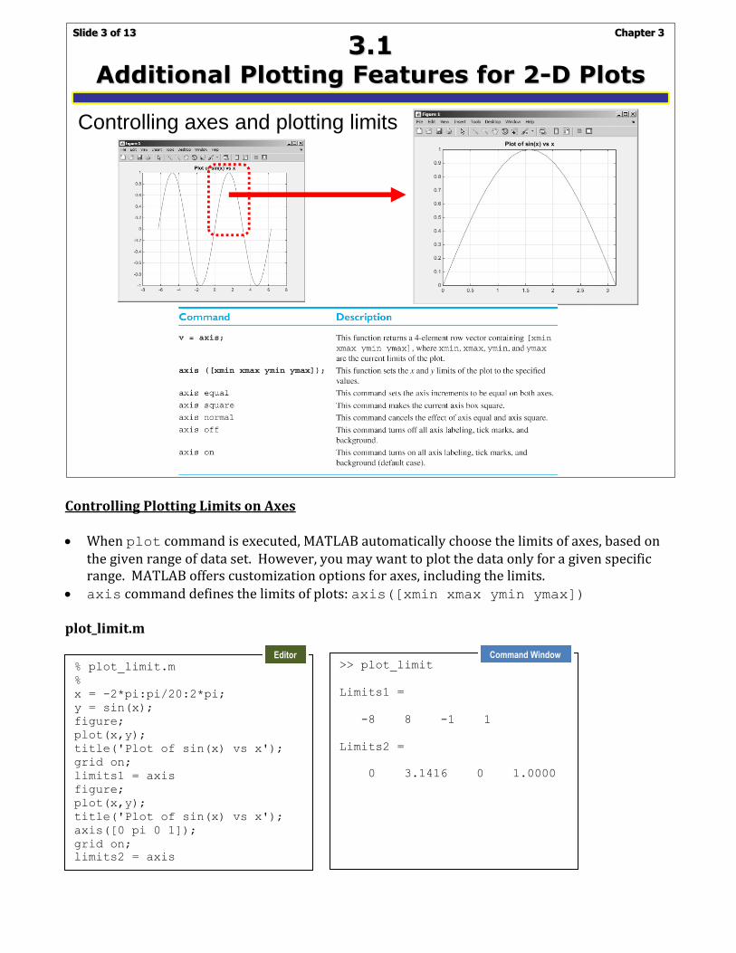
Controlling Plotting Limits on Axes When plot command is executed, MATLAB automatically choose the limits of axes, based on

the given range of data set. However, you may want to plot the data only for a given specific range. MATLAB offers customization options for axes, including the limits.

axis command defines the limits of plots: axis([xmin xmax ymin ymax]) plot_limit.m



Controlling axes and plotting limits

% plot_limit.m

%

x = -2*pi:pi/20:2*pi;

y = sin(x);

figure;

plot(x,y);

title('Plot of sin(x) vs x');

grid on;

limits1 = axis

figure;

plot(x,y);

title('Plot of sin(x) vs x');

axis([0 pi 0 1]);

grid on;

limits2 = axis

>> plot_limit

Limits1 =

-8 8 -1 1

Limits2 =

0 3.1416 0 1.0000

Editor Command Window

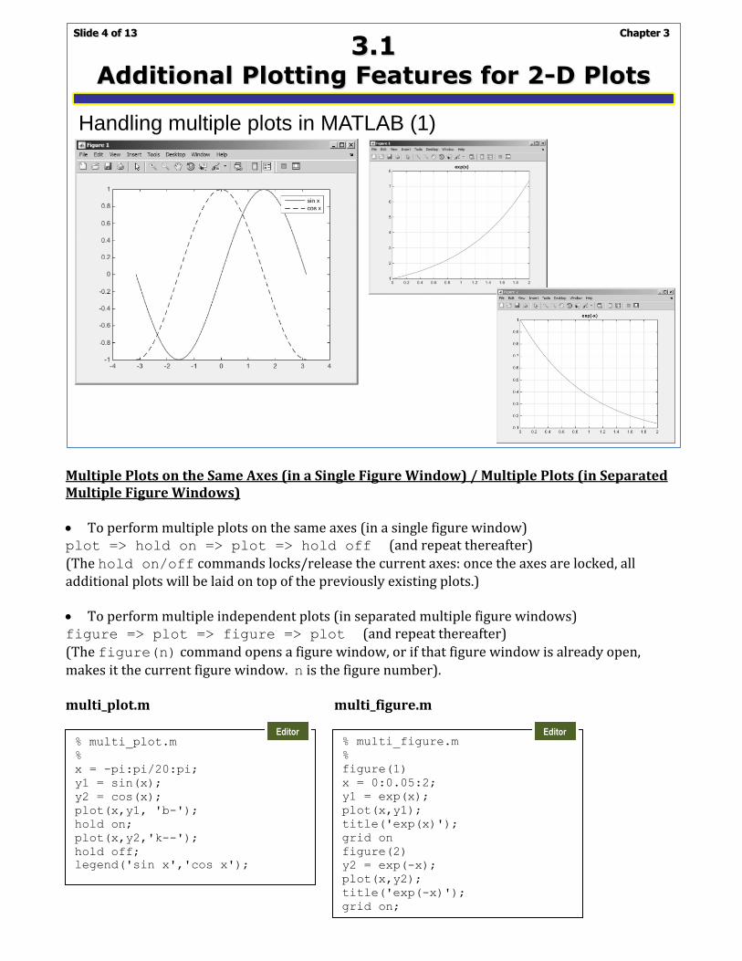
% multi_figure.m

%

figure(1)

x = 0:0.05:2;

y1 = exp(x);

plot(x,y1);

title('exp(x)');

grid on

figure(2)

y2 = exp(-x);

plot(x,y2);

title('exp(-x)');

grid on;

Multiple Plots on the Same Axes (in a Single Figure Window) / Multiple Plots (in Separated Multiple Figure Windows) To perform multiple plots on the same axes (in a single figure window) plot => hold on => plot => hold off (and repeat thereafter) (The hold on/off commands locks/release the current axes: once the axes are locked, all additional plots will be laid on top of the previously existing plots.) To perform multiple independent plots (in separated multiple figure windows) figure => plot => figure => plot (and repeat thereafter) (The figure(n) command opens a figure window, or if that figure window is already open, makes it the current figure window. n is the figure number). multi_plot.m multi_figure.m



Handling multiple plots in MATLAB (1)

% multi_plot.m

%

x = -pi:pi/20:pi;

y1 = sin(x);

y2 = cos(x);

plot(x,y1, 'b-');

hold on;

plot(x,y2,'k--');

hold off;

legend('sin x','cos x');

Editor Editor

Subplots It is possible to place more than one set of axes on a single figure, creating multiple subplots:

subplot(m,n,p) divides the current figure into m by n equal-sized regions, arranged in m rows and n columns, and creates a set of axes at position p to receive all current plotting commands.

subplot(2,3,4) opens a new figure, divides it to six regions arranged in two rows and three columns and create an axis in position four (the lower left).

Controlling the Data Points (Limits and Number of Points) It is often not easy to identify “how many” data points will be in array. Also, there is no guarantee that last specified point will be in the array (since the increment may “overshoot” that point). There is actually a very effective way to control the exact limit and number of points of the array: linspace(start,end) / linspace(start,end,n)

logspace(start,end) / logspace(start,end,n)

create_subplots.m



Handling multiple plots in MATLAB (2)

Position 1 Position 2 Position 3

Position 5 Position 6Position 4

% create_subplots.m

%

figure(1)

subplot(2,1,1)

x = -pi:pi/20:pi;

y = sin(x);

plot(x,y);

title('Subplot 1 title');

subplot(2,1,2)

x = -pi:pi/20:pi;

y = cos(x);

plot(x,y);

title('Subplot 2 title');

>> linspace(1,10,10)

ans =

1 2 3 4 5 6 7 8 9 10

>> logspace(0,1,5)

ans =

1.0000 1.7783 3.1623 5.6234 10.0000

Editor Command Window

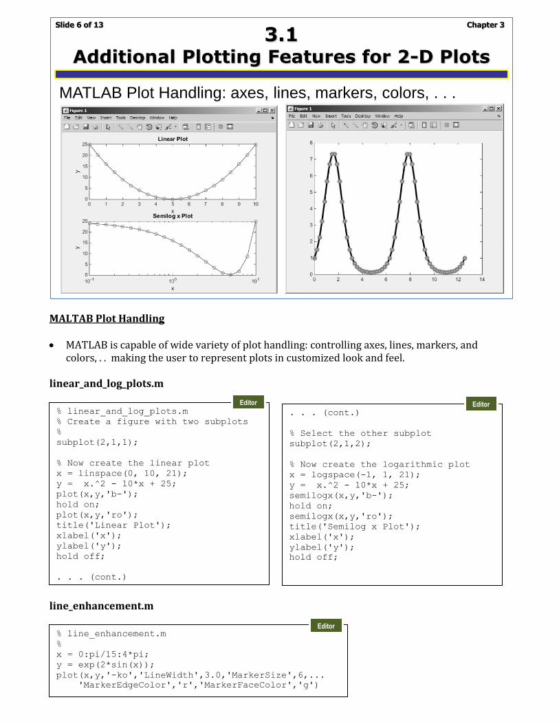
MALTAB Plot Handling MATLAB is capable of wide variety of plot handling: controlling axes, lines, markers, and

colors, . . making the user to represent plots in customized look and feel. linear_and_log_plots.m

line_enhancement.m



MATLAB Plot Handling: axes, lines, markers, colors, . . .

% linear_and_log_plots.m

% Create a figure with two subplots

%

subplot(2,1,1);

% Now create the linear plot

x = linspace(0, 10, 21);

y = x.^2 - 10*x + 25;

plot(x,y,'b-');

hold on;

plot(x,y,'ro');

title('Linear Plot');

xlabel('x');

ylabel('y');

hold off;

. . . (cont.)

. . . (cont.)

% Select the other subplot

subplot(2,1,2);

% Now create the logarithmic plot

x = logspace(-1, 1, 21);

y = x.^2 - 10*x + 25;

semilogx(x,y,'b-');

hold on;

semilogx(x,y,'ro');

title('Semilog x Plot');

xlabel('x');

ylabel('y');

hold off;

% line_enhancement.m

%

x = 0:pi/15:4*pi;

y = exp(2*sin(x));

plot(x,y,'-ko','LineWidth',3.0,'MarkerSize',6,...

'MarkerEdgeColor','r','MarkerFaceColor','g')

Editor Editor

Editor

Enhanced Control of Plotted Lines In MATLAB plots, it is also possible to set additional properties with each line: Linewidth

(specifies the width of each line in points), MarkerEdgeColor (specifies the color of the marker or the edge color for filled markers), MarkerFaceColor (specifies the color of the face of filled

markers), and MarkerSize (specifies the size of the marker in points). These properties can be specified by: plot(x,y,’PropertyName’,value,...) Specifier Definitions Line Style: - (solid line: default) -- (dashed line) : (dotted line) -. (dash-dot line)

Marker: o (circle) + (plus sign) * (asterisk) . (point) x (cross) s (square) d (diamond)

^ (upward-pointing triangle) v (downward-pointing triangle) > (right-pointing triangle) < (left-pointing triangle) p (pentagon) h (hexagon)

Color: y (yellow) m (magenta) c (cyan) r (red) g (green) b (blue) w (white) k (black) MATLAB is also capable of controlling texts in plots (special symbols, characters, etc.). special_symbols.m



Enhanced control of texts

\tau_{ind} versus \omega_{\itm} => \theta varies from 0\circ to 90\circ =>

\bf{B}_{\itS} => BS

% special_symbols.m

tau = 3;

omega = pi;

t = linspace(0, 10, 100);

y = 10 * exp(-t./tau) .* sin(omega .* t);;

plot(t,y,'b-');

title('Plot of \it{y(t)} = \it{e}^{-\it{t / \tau}} sin \it{\omegat}');

xlabel('\it{t}');

ylabel('\it{y(t)}');

grid on;

Editor

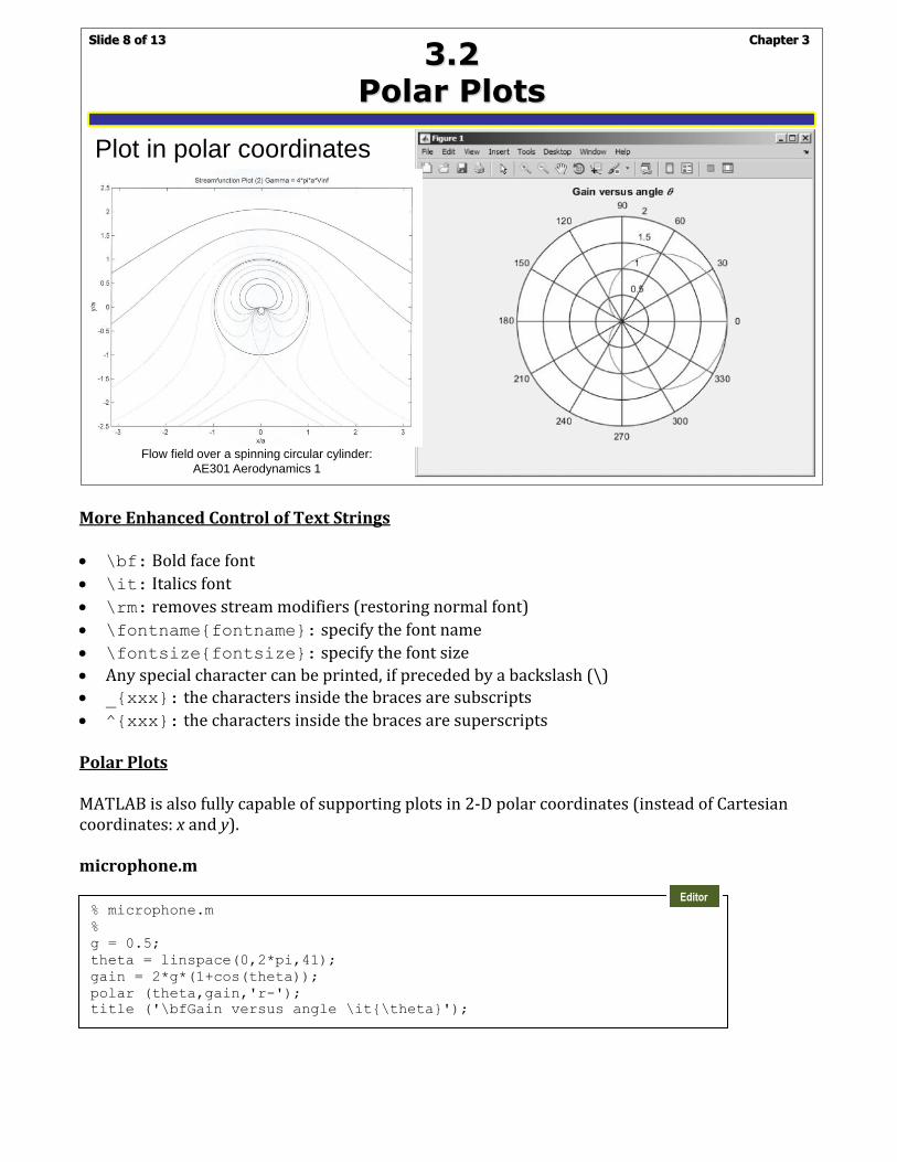
More Enhanced Control of Text Strings \bf: Bold face font

\it: Italics font

\rm: removes stream modifiers (restoring normal font)

\fontname{fontname}: specify the font name

\fontsize{fontsize}: specify the font size

Any special character can be printed, if preceded by a backslash (\)

_{xxx}: the characters inside the braces are subscripts

^{xxx}: the characters inside the braces are superscripts Polar Plots MATLAB is also fully capable of supporting plots in 2-D polar coordinates (instead of Cartesian coordinates: x and y). microphone.m


3.2 Polar Plots

Plot in polar coordinates

Flow field over a spinning circular cylinder:

AE301 Aerodynamics 1

% microphone.m

%

g = 0.5;

theta = linspace(0,2*pi,41);

gain = 2*g*(1+cos(theta));

polar (theta,gain,'r-');

title ('\bfGain versus angle \it{\theta}');

Editor

MATLAB Figure Window Once a plot is created in MATLAB, you can edit and annotate the plot within the figure window. Many GUI-based plot handling tools are available (plot toolbar in MATLAB figure window). Plot Toolbar (MATLAB Figure Window) Using the plot toolbar within each MATLAB figure window, you can: Open/close, save, import/export, and print your plot Edit graphical properties Insert axis labels, title, legend, colorbar, custom-shapes, and texts Control the viewing of plot (pan, zoom, rotate, etc.) After executing the MATLAB script “microphone.m,” try handling/manipulating the plot & figure using the plot toolbar. For example:

Zoom in/out, pan, & rotate the plot Insert axis labels, line, arrow, text arrow, & text box in the plot Copy & paste the figure Save the figure Print the figure



Plot in polar coordinates

exercise_3_1.m



Do-It-Yourself (DIY) EXERCISE 3-1

(a) Write the MATLAB text string that will produce the following expression:

(b) Write the expression produced by the following text strings:’\tau\it_{m}’

’\bf\itx_{1}^{ 2} + x_{2}^{ 2} \rm(units:\bfm^{2}\rm)’

(c) Plot the function r = 10*cos(3 ) for 0 2 (increment of 0.01) using a polar plot.

(d) Plot the function for 0.01 x 100 on a linear and log/log plot. 2

1

2y x

x

(Take advantage of linspace and logspace when creating the plots)

sin cos2f x

% exercise_3_1.m

%

%(a)

figure

theta = -pi:pi/20:pi;

phi = 0:pi/20:2*pi;

y = sin(theta).*cos(2*phi);

plot(theta,y);

title('\itf\rm(\itx\rm) = sin \theta cos 2\phi');

%(b)

ylabel('\tau\it_{m}');

xlabel('\bf\itx_{1}^{ 2} + x_{2}^{ 2} \rm(units:\bfm^{2}\rm)');

%(c)

clear

theta = 0:0.01*pi:2*pi;

r = 10*cos(3.*theta);

figure

polar(theta,r);

%(d)

clear

x1 = linspace(0.01,100,100);

x2 = logspace(0.01,100,100);

y1 = 1./(2.*x1.^2);

y2 = 1./(2.*x2.^2);

figure

subplot(2,1,1);

plot(x1,y1);

title('Linear Plot')

grid on

subplot(2,1,2);

loglog(x2,y2);

title('Log-Log Plot')

grid on

Editor _________________________________________________________

_________________________________________________________

_________________________________________________________

_________________________________________________________

_________________________________________________________

_________________________________________________________

_________________________________________________________

_________________________________________________________

_________________________________________________________

_________________________________________________________

_________________________________________________________

_________________________________________________________

_________________________________________________________

_________________________________________________________

_________________________________________________________

_________________________________________________________

_________________________________________________________

_________________________________________________________

_________________________________________________________

_________________________________________________________

_________________________________________________________

_________________________________________________________

exercise_3_2.m



Do-It-Yourself (DIY) EXERCISE 3-2

(a) Develop a MATLAB statement to plot sin(x) versus cos(2x) for the range of xfrom 0 to 2 (increment of /10). The points should be connected by a 2-pixel-wide solid red line, and each point should be marked with 7-pixel-wide blue diamond marker with green edge.

(b) Use the figure editing tools to change the markers into black square with yellow edge. Also, using the figure editing tools, add an arrow and annotation pointing to the location x = on the plot.

% exercise_3_2.m

%

%(a)

x = 0:pi/10:2*pi;

y1 = sin(x);

y2 = cos(2.*x);

plot(y1,y2,'-rd','Linewidth',1,'Markersize',7,...

'MarkerEdgeColor','g','MarkerFaceColor','b');

grid on;

title('sin(x) vs cos(2x)');

xlabel('sin(x)');

ylabel('cos(2x)');

Editor _________________________________________________________

_________________________________________________________

_________________________________________________________

_________________________________________________________

_________________________________________________________

_________________________________________________________

_________________________________________________________

_________________________________________________________

_________________________________________________________

_________________________________________________________

_________________________________________________________

_________________________________________________________

_________________________________________________________

_________________________________________________________

_________________________________________________________

_________________________________________________________

_________________________________________________________

_________________________________________________________

_________________________________________________________

_________________________________________________________

_________________________________________________________

_________________________________________________________

_________________________________________________________

_________________________________________________________

_________________________________________________________

Additional MATLAB 2-D Specialized Plots MATLAB supports many other more specialized plots: Stem plots Stair plots Bar plots Pie charts Compass plots (type lookfor plot in Command Window to see the variety of MATLAB plot features)


3.4 Additional Types of 2-D Plots

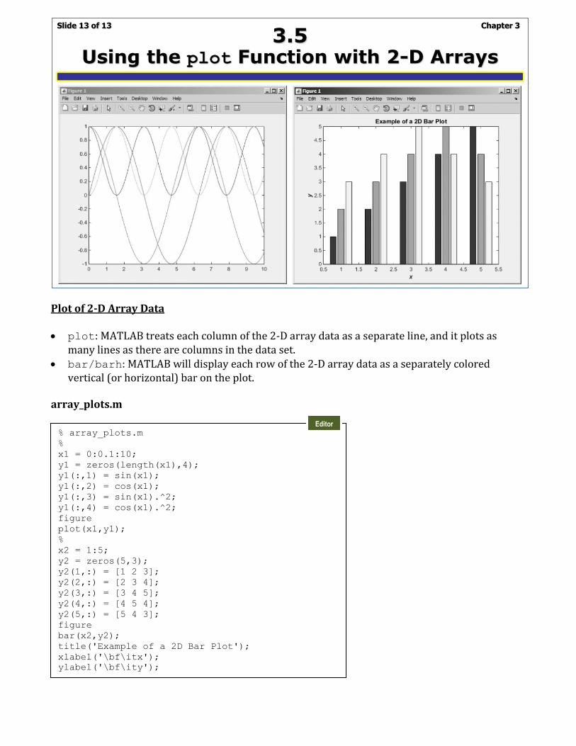
Plot of 2-D Array Data plot: MATLAB treats each column of the 2-D array data as a separate line, and it plots as

many lines as there are columns in the data set. bar/barh: MATLAB will display each row of the 2-D array data as a separately colored

vertical (or horizontal) bar on the plot. array_plots.m


3.5 Using the plot Function with 2-D Arrays

% array_plots.m

%

x1 = 0:0.1:10;

y1 = zeros(length(x1),4);

y1(:,1) = sin(x1);

y1(:,2) = cos(x1);

y1(:,3) = sin(x1).^2;

y1(:,4) = cos(x1).^2;

figure

plot(x1,y1);

%

x2 = 1:5;

y2 = zeros(5,3);

y2(1,:) = [1 2 3];

y2(2,:) = [2 3 4];

y2(3,:) = [3 4 5];

y2(4,:) = [4 5 4];

y2(5,:) = [5 4 3];

figure

bar(x2,y2);

title('Example of a 2D Bar Plot');

xlabel('\bf\itx');

ylabel('\bf\ity');

Editor

Date post:	02-Jul-2018
Category:	Documents
Upload:	vannguyet
View:	215 times
Download:	0 times

3.4 Additional Types of 2 - D Plots 3.5 Using the 3.2...

Documents