19
3.4 Velocity and Rates of Change
| Date post: | 24-Dec-2015 |
| Category: |
Documents |
| Upload: | byron-sherman |
| View: | 218 times |
| Download: | 0 times |

3.4 Velocity and Rates of Change
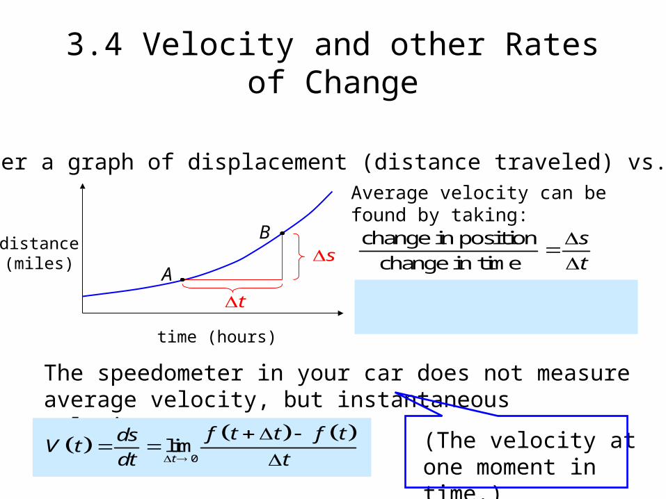
Consider a graph of displacement (distance traveled) vs. time.
time (hours)
distance(miles)
Average velocity can be found by taking:change in position
change in time
s
t
t
sA
B
ave
f t t f tsV
t t
The speedometer in your car does not measure average velocity, but instantaneous velocity.
0
limt
f t t f tdsV t
dt t
(The velocity at one moment in time.)
3.4 Velocity and other Rates of Change
3.4 Velocity and other Rates of Change
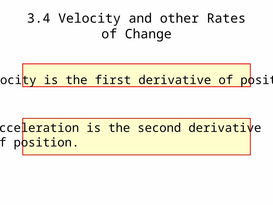
Velocity is the first derivative of position.
Acceleration is the second derivative of position.

Example: Free Fall Equation
21
2s g t
GravitationalConstants:
2
ft32
secg
2
m9.8
secg
2
cm980
secg
2132
2s t
216 s t 32 ds
V tdt
Speed is the absolute value of velocity.
3.4 Velocity and other Rates of Change

Acceleration is the derivative of velocity.
dva
dt
2
2
d s
dt example:
32v t
32a If distance is in: feet
Velocity would be in:feet
sec
Acceleration would be in:
ftsec sec
2
ft
sec
3.4 Velocity and other Rates of Change

time
distance
acc posvel pos &increasing
acc zerovel pos &constant
acc negvel pos &decreasing
velocityzero
acc negvel neg &decreasing acc zero
vel neg &constant
acc posvel neg &increasing
acc zero,velocity zero
3.4 Velocity and other Rates of Change

Rates of Change:
Average rate of change = f x h f x
h
Instantaneous rate of change = 0
limh
f x h f xf x
h
These definitions are true for any function.
( x does not have to represent time. )
3.4 Velocity and other Rates of Change

For a circle: 2A r2dA dr
dr dr
2dA
rdr
Instantaneous rate of change of the area withrespect to the radius.
For tree ring growth, if the change in area is constant then dr must get smaller as r gets larger.
2 dA r dr
3.4 Velocity and other Rates of Change

Evaluate the rate of change of the area of a circle A at r = 5 and r = 10.

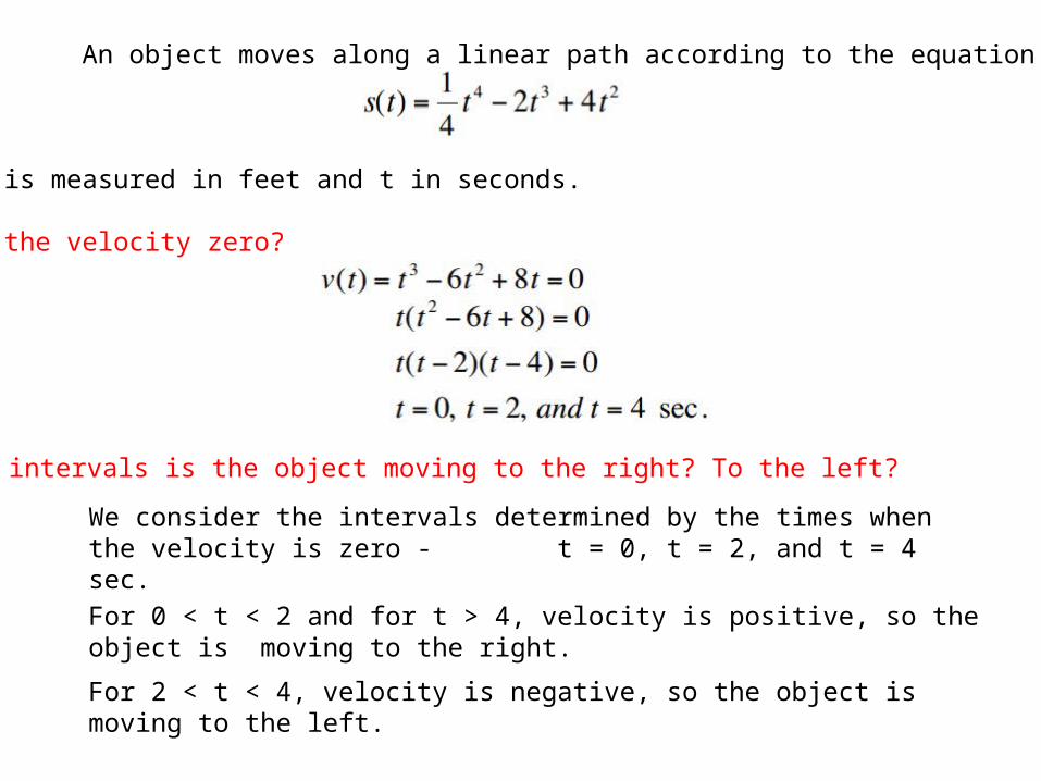
EXAMPLE: An object moves along a linear path according to the equation
where s is measured in feet and t in seconds.
Determine its velocity when t = 4 and when t = 2.
When is the velocity zero?

EXAMPLE: An object moves along a linear path according to the equation
where s is measured in feet and t in seconds.
Determine its position, velocity, and acceleration when t = 0 and when t = 3 seconds.
EXAMPLE: An object moves along a linear path according to the equation
where s is measured in feet and t in seconds.
When is the velocity zero?
On what intervals is the object moving to the right? To the left?
We consider the intervals determined by the times when the velocity is zero - t = 0, t = 2, and t = 4 sec.
For 0 < t < 2 and for t > 4, velocity is positive, so the object is moving to the right.
For 2 < t < 4, velocity is negative, so the object is moving to the left.

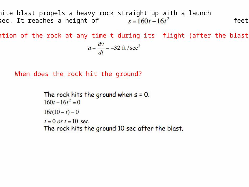
EXAMPLE: A dynamite blast propels a heavy rock straight up with a launchvelocity of 160 ft/sec. It reaches a height of feet after t seconds.
How high does the rock go?

What is the velocity and speed of the rock when it is 256 ft above the ground on the way up? on the way down?
EXAMPLE: A dynamite blast propels a heavy rock straight up with a launchvelocity of 160 ft/sec. It reaches a height of feet after t seconds.
EXAMPLE: A dynamite blast propels a heavy rock straight up with a launchvelocity of 160 ft/sec. It reaches a height of feet after t seconds.
What is the acceleration of the rock at any time t during its flight (after the blast)?
When does the rock hit the ground?

from Economics:
Marginal cost is the first derivative of the cost function, and represents an approximation of the cost of producing one more unit.
3.4 Velocity and other Rates of Change

Example 13:Suppose it costs: 3 26 15c x x x x
to produce x stoves. 23 12 15c x x x
If you are currently producing 10 stoves, the 11th stove will cost approximately:
210 3 10 12 10 15c 300 120 15
$195marginal cost
The actual cost is: 11 10C C
3 2 3 211 6 11 15 11 10 6 10 15 10
770 550 $220 actual cost
3.4 Velocity and other Rates of Change

Note that this is not a great approximation – Don’t let that bother you.
Marginal cost is a linear approximation of a curved function. For large values it gives a good approximation of the cost of producing the next item.
3.4 Velocity and other Rates of Change

HOMEWORK
• P. 135-137 • #1-4, 9-20


