36 Small and medium-sized industry in Turkey40 Small and medium-sized industry in Turkey T able 3.5...

36 Small and medium-sized industry in Turkey

31 Food and tobacco 85 85 –8702 32 Textile 93 87 53455 33 Wood products 44 47 975 34 Paper products 80 87 –2096 35 Chemicals 87 100 6191 36 Non-metallic mineral products 105 82 –887 37 Basic metal 166 168 –9715 38 Engineering 80 85 10336 39 Other manufacturing 46 49 –415 3 Manufacturing 88 88 49142

The shift in the size distribution has been accompanied by a structural change in the composition of employment. The share of employees, i.e., wage labour, has increased continuously as a result of the dissolution of traditional sectors. The share of non-wage labour (owners and unpaid family members) dropped from 33.2% in 1963 to 16.6% in 1992. The transformation of the family labour reflects the increased penetration of capitalist relations in manufacturing industry.

Table 3.3 and 3.4 presents the data on APS in Turkish manufacturing sector at the 2-digit industry level in 1985 and 1992 (see Tables 3.5-3.7 for data at the 4-digit industry level). The APS in these tables does not include micro establishments.

There are significant inter-industry differences in APS. The lowest APS is found in the wood products industry (ISIC 33) in which the APS is 47 employees, whereas a typical establishment in the basic metal industry (ISIC 37) employs 168 people. The APS at the 2-digit industry level does not show any significant change from 1985 to 1992 with the exception of the non-metallic mineral products industry (ISIC 36).* There seems to be no correlation between net change in employment in the sector and the change in APS.

The APS in the public and private sectors is shown in Table 3.4. An average public enterprise is much larger than a private enterprise in the same sector. The

* ISIC Classification refers to International Standard Industry Classification, Rev. 2.

Determinants of average plant size 37 difference is most obvious in the basic metal industry in which typical public and private establishments employ 2971 and 72 persons respectively. The public establishments are large because i) employment creation is one of the implicit objectives of the public sector, and ii) the degree of vertical integration is higher in public establishments.

A sharp decline in APS is observed in the public sector, from 704 in 1985 to 539 in 1992, as a result of serious employment loss in public establishments. The APS tends to increase slightly in the private sector, from 65 in 1985 to 70 in 1992.

A typical new establishment is smaller than the incumbent in all sectors. (There are only a few exceptions at the 4-digit industry level. See Tables 3.6 and 3.7.) This proves that new establishments start small because of imperfect capital markets and/or the risks involved with entry to a new business. The dynamics of entry and growth will be analyzed in detail in Chapter 6.

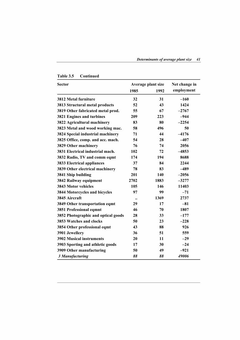
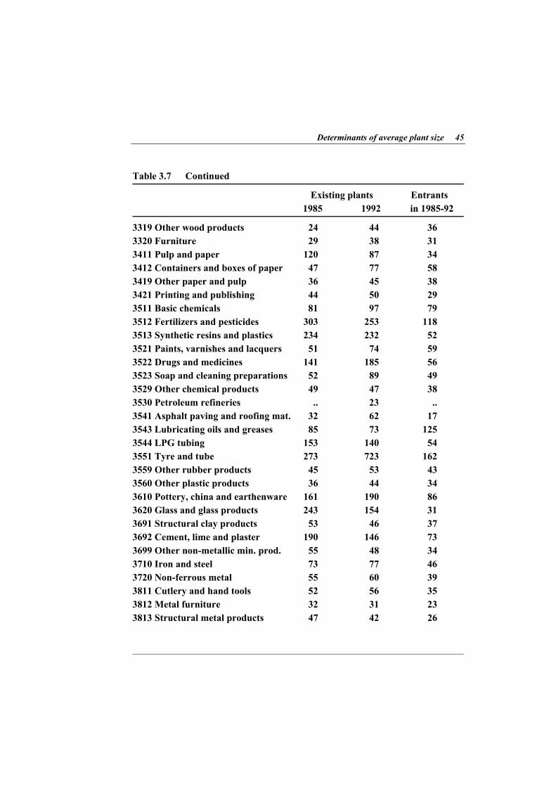
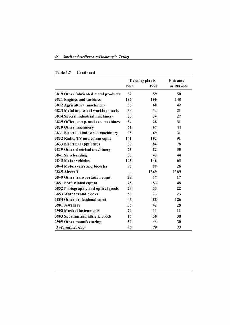
Tables 3.5-3.7 present the data on average plant size at the 4-digit industry level. In 1992, the highest APS is found for the iron and steel industry (3763 employees) whereas the smallest one for the paint, varnish and lacquer industry (only 14 employees). In the private sector, the highest and lowest figures are found for the aircraft (1369 employees) and musical instruments (11 employees) industries. The data show that there are significant and persistent differences in APS across industries. Policy makers should understand the factors behind inter-industry differences in APS, because these factors explain why SMEs are more successful in some industries. For this reason, the determinants of APS will be analyzed in the next sub-section to shed light on the industrial characteristics that create a suitable environment for SME development.

38 Small and medium-sized industry in Turkey T able 3.4 Average plant size (2-digit industries), 1985 and 1992

Existing plants Entrants 1985 1992 in 1985-92

Public sector 31 Food and tobacco 462 343 188 32 Textile 1097 809 722 33 Wood products 254 220 72 34 Paper products 829 683 .. 35 Chemicals 937 751 411 36 Non-metallic mineral products 420 358 308 37 Basic metal 3775 2971 1288 38 Engineering 907 643 222 39 Other manufacturing .. 336 247 3 Manufacturing 704 539 313

Private sector 31 Food and tobacco 47 56 39 32 Textile 80 79 46 33 Wood products 33 38 30 34 Paper products 47 60 35 35 Chemicals 65 77 42 36 Non-metallic mineral products 90 72 40 37 Basic metal 67 72 44 38 Engineering 65 76 46 39 Other manufacturing 46 43 29 3 Manufacturing 65 70 43

Determinants of average plant size 39

Table 3.5 Average plant size in 1985 and 1992, and net change in employment n the period 1985 to 1992 (4-digit industries) i

Sector Average plant size Net change in 1985 1992 employment

3111 Meat 118 115 3366 3112 Dairy products 48 50 1309 3113 Fruits and vegetables 123 129 4265 3114 Fish crustacea 63 106 1146 3115 Oils and fats 102 98 –2555 3116 Grain mill products 31 27 –1660 3117 Bakery products 24 26 –4575 3118 Sugar 1166 808 –606 3119 Confectionery 45 84 3150 3121 Other food products 177 120 –1343 3122 Animal feeds 51 40 228 3131 Spirits 297 314 1082 3132 Wine 45 56 –310 3133 Malt liquors and malt 428 353 –1028 3134 Non-alcoholic beverages 84 109 1865 3140 Tobacco 818 645 –13036 3211 Spinning and weaving 181 167 –17374 3212 Textile exc. wearing apparel 66 83 6466 3213 Knitting 45 85 19718 3214 Carpets and rugs 121 100 –2146 3215 Cordage rope 45 51 –341 3219 Other textile products 74 45 –1550 3221 Fur and leather products 50 49 6018 3222 Wearing apparel 44 55 42690 3231 Leather finishing 33 45 –725 3232 Fur dressing .. 27 54 3233 Other leather 32 59 1366 3240 Footwear 50 43 –721 3311 Sawmills and planing 58 57 –71


T able 3.5 Continued


3312 Wooden and cane containers 34 15 –378 3319 Other wood products 24 44 247 3320 Furniture 30 38 1177 3411 Pulp and paper 480 233 –437 3412 Containers and boxes of paper 65 77 –455 3419 Other paper and pulp 36 45 –1029 3421 Printing and publishing 51 57 –175 3511 Basic chemicals 120 327 7510 3512 Fertilizers and pesticides 542 340 –4847 3513 Synthetic resins and plastics 488 241 –7424 3521 Paints, varnishes and lacquers 54 73 –314 3522 Drugs and medicines 145 188 2074 3523 Soap and cleaning preparations 52 89 1093 3529 Other chemical products 75 63 464 3530 Petroleum refineries 981 828 1040 3541 Asphalt paving and roofing mat. 32 172 306 3542 Coke coal and briquettes 58 57 –59 3543 Lubricating oils and greases 118 122 –59 3544 LPG tubing 153 140 –19 3551 Tyre and tube 273 731 1849 3559 Other rubber products 45 53 163 3560 Other plastic products 36 44 4414 3610 Pottery, china and earthenware 192 215 –1444 3620 Glass and glass products 243 161 –1789 3691 Structural clay products 58 49 1145 3692 Cement, lime and plaster 233 171 –1321 3699 Other non-metallic min. prod. 63 53 2522 3710 Iron and steel 185 188 –2020 3720 Non-ferrous metal 131 119 –7695 3811 Cutlery and hand tools 52 56 941




3812 Metal furniture 32 31 –160 3813 Structural metal products 52 43 1424 3819 Other fabricated metal prod. 55 67 –2767 3821 Engines and turbines 209 223 –944 3822 Agricultural machinery 83 80 –2254 3823 Metal and wood working mac. 58 496 50 3824 Special industrial machinery 71 44 –4176 3825 Office, comp. and acc. mach. 54 28 –407 3829 Other machinery 76 74 2056 3831 Electrical industrial mach. 102 72 –4853 3832 Radio, TV and comm eqmt 174 194 8688 3833 Electrical appliances 37 84 2244 3839 Other electrical machinery 78 83 –489 3841 Ship building 201 140 –2056 3842 Railway equipment 2702 1883 –3277 3843 Motor vehicles 105 146 11403 3844 Motorcycles and bicycles 97 99 –71 3845 Aircraft .. 1369 2737 3849 Other transportation eqmt 29 17 –81 3851 Professional eqmnt 46 70 1807 3852 Photographic and optical goods 28 33 –177 3853 Watches and clocks 50 23 –228 3854 Other professional eqmt 43 88 926 3901 Jewellery 36 51 559 3902 Musical instruments 20 11 –29 3903 Sporting and athletic goods 17 30 –24 3909 Other manufacturing 50 49 –921 3 Manufacturing 88 88 49006


Table 3.6 Average plant size in the public sector (4-digit industries), 1985 and 992 1


3111 Meat 236 175 75 3112 Dairy products 56 52 25 3114 Fish crustacea .. 144 .. 3115 Oils and fats 125 181 85 3116 Grain mill products 86 90 .. 3117 Bakery products 128 87 18 3118 Sugar 1158 940 648 3121 Other food products 442 336 .. 3122 Animal feeds 63 52 41 3131 Spirits 297 314 128 3132 Wine 72 46 .. 3133 Malt liquors and malt 566 384 .. 3134 Non-alcoholic beverages 80 45 18 3140 Tobacco 1439 1014 1454 3211 Spinning and weaving 1217 997 872 3212 Textile exc. wearing apparel .. 306 .. 3214 Carpets and rugs 423 277 122 3222 Wearing apparel 221 721 .. 3231 Leather finishing .. 1460 .. 3240 Footwear 738 338 .. 3311 Sawmills and planing 266 220 72 3312 Wooden and cane containers 153 .. .. 3320 Furniture 101 .. .. 3411 Pulp and paper 1470 1180 .. 3412 Containers and boxes of paper 575 .. .. 3421 Printing and publishing 282 241 .. 3511 Basic chemicals 654 1377 78 3512 Fertilizers and pesticides 1209 718 .. 3513 Synthetic resins and plastics 2613 338 81 3521 Paints, varnishes and lacquers 268 14 ..




3522 Drugs and medicines 283 291 .. 3523 Soap and cleaning preparations .. 117 .. 3529 Other chemical products 595 390 147 3530 Petroleum refineries 981 988 1151 3541 Asphalt paving and roofing mat. .. 499 499 3542 Coke coal and briquettes 58 57 .. 3543 Lubricating oils and greases 539 393 328 3551 Tyre and tube .. 780 780 3560 Other plastic products .. 225 225 3610 Pottery, china and earthenware 759 564 .. 3620 Glass and glass products .. 636 636 3691 Structural clay products 896 652 .. 3692 Cement, lime and plaster 347 273 210 3699 Other non-metallic min. prod. 318 368 373 3710 Iron and steel 5092 3763 1288 3720 Non-ferrous metal 2239 1545 .. 3813 Structural metal products 850 297 .. 3819 Other fabricated metal products 423 705 .. 3821 Engines and turbines 452 363 .. 3822 Agricultural machinery 490 337 76 3823 Metal and wood working mach. 807 801 .. 3824 Special industrial machinery 501 409 .. 3829 Other machinery 2560 726 323 3831 Electrical industrial mach. 570 194 194 3832 Radio, TV and comm eqmt 1214 383 .. 3839 Other electrical machinery 299 170 .. 3841 Ship building 1018 945 .. 3842 Railway equipment 2702 1883 .. 3851 Professional eqmnt 480 421 .. 3901 Jewellery .. 247 247 3909 Other manufacturing .. 425 .. 3 Manufacturing 704 539 313


Table 3.7 Average plant size in the private sector (4-digit industries), 1985 and 992 1


3111 Meat 52 88 71 3112 Dairy products 43 50 27 3113 Fruits and vegetables 123 129 109 3114 Fish crustacea 63 104 139 3115 Oils and fats 100 95 45 3116 Grain mill products 31 27 20 3117 Bakery products 24 26 19 3118 Sugar 1192 486 13 3119 Confectionary 45 84 33 3121 Other food products 64 62 52 3122 Animal feeds 48 38 35 3132 Wine 29 65 28 3133 Malt liquors and malt 359 342 .. 3134 Non-alcoholic beverages 85 117 98 3140 Tobacco 173 225 185 3211 Spinning and weaving 149 143 74 3212 Textile exc. wearing apparel 66 78 52 3213 Knitting 45 85 50 3214 Carpets and rugs 117 94 41 3215 Cordage rope 45 51 .. 3219 Other textile products 74 45 40 3221 Fur and leather products 50 49 38 3222 Wearing apparel 43 54 41 3231 Leather finishing 33 33 25 3232 Fur dressing .. 27 27 3233 Other leather 32 59 35 3240 Footwear 29 36 30 3311 Sawmills and planing 38 40 30 3312 Wooden and cane containers 27 15 15

Determinants of average plant size 45 T able 3.7 Continued


3319 Other wood products 24 44 36 3320 Furniture 29 38 31 3411 Pulp and paper 120 87 34 3412 Containers and boxes of paper 47 77 58 3419 Other paper and pulp 36 45 38 3421 Printing and publishing 44 50 29 3511 Basic chemicals 81 97 79 3512 Fertilizers and pesticides 303 253 118 3513 Synthetic resins and plastics 234 232 52 3521 Paints, varnishes and lacquers 51 74 59 3522 Drugs and medicines 141 185 56 3523 Soap and cleaning preparations 52 89 49 3529 Other chemical products 49 47 38 3530 Petroleum refineries .. 23 .. 3541 Asphalt paving and roofing mat. 32 62 17 3543 Lubricating oils and greases 85 73 125 3544 LPG tubing 153 140 54 3551 Tyre and tube 273 723 162 3559 Other rubber products 45 53 43 3560 Other plastic products 36 44 34 3610 Pottery, china and earthenware 161 190 86 3620 Glass and glass products 243 154 31 3691 Structural clay products 53 46 37 3692 Cement, lime and plaster 190 146 73 3699 Other non-metallic min. prod. 55 48 34 3710 Iron and steel 73 77 46 3720 Non-ferrous metal 55 60 39 3811 Cutlery and hand tools 52 56 35 3812 Metal furniture 32 31 23 3813 Structural metal products 47 42 26




3819 Other fabricated metal products 52 59 50 3821 Engines and turbines 186 166 148 3822 Agricultural machinery 55 60 42 3823 Metal and wood working mach. 39 34 21 3824 Special industrial machinery 55 34 27 3825 Office, comp. and acc. machines 54 28 31 3829 Other machinery 61 67 44 3831 Electrical industrial machinery 95 69 31 3832 Radio, TV and comm eqmt 141 192 91 3833 Electrical appliances 37 84 78 3839 Other electrical machinery 75 82 35 3841 Ship building 37 42 44 3843 Motor vehicles 105 146 63 3844 Motorcycles and bicycles 97 99 26 3845 Aircraft .. 1369 1369 3849 Other transportation eqmt 29 17 17 3851 Professional eqmnt 28 53 48 3852 Photographic and optical goods 28 33 22 3853 Watches and clocks 50 23 23 3854 Other professional eqmt 43 88 126 3901 Jewellery 36 42 28 3902 Musical instruments 20 11 11 3903 Sporting and athletic goods 17 30 38 3909 Other manufacturing 50 44 30 3 Manufacturing 65 70 43

Determinants of average plant size 47 3.3 Determinants of average plant size: An econometric analysis APS is a measure of the share (and role) of SMEs in that sector: the lower the APS, the higher the share of SMEs. There are some structural factors that determine the level of sectoral APS. The first set of factors is related to production technology. If there are economies of scale in production, plants will increase the volume of output to reduce unit production cost. The level of output where economies of scale are exhausted is called the "minimum efficient scale". The unit production cost is minimized at the minimum efficient scale. Competition in the market will force firms to produce efficiently, i.e., at the minimum efficient scale. Thus the minimum efficient scale determines the size of an establishment: the higher the minimum efficient scale, the larger the plant size.

Product differentiation is an important aspect of the market structure. If firms produce a range of differentiated products, they will have a larger size, ceteris paribus. The type of technology determines the plant size. If production requires a large initial fixed investment, and if the capital markets are not perfect, potential small firms who are willing to enter into that sector will be discouraged. New firms could prefer to enter into those sectors in which the sunk cost of investment is low.

These factors are structural in the sense that they are determined by available product and process technologies. The structural conditions set the rules of the game. Any size distribution could be considered as "acceptable" or even "desirable" because it is evolved through the "rational" behaviour of firms operating under certain technological constraints. For example, LSEs dominate the iron and steel industry because the available technology dictates the formation of LSEs. If this is the case, the policy aimed to promote SMEs will be helpless if it is not directed towards changing the underlying structural factors.

The second set of factors is related to the strategic behaviour of firms and the institutional framework imposed by the state. Firms can establish monopolistic power by strategic behaviour. For example, incumbent firms may raise entry barriers by forcing new (small) firms to spend extensively in non-production activities like advertising and marketing. Institutional factors, especially those which are related to the labour market, should also be taken into consideration. If wages are determined at the establishment level, less productive firms tend to pay lower wages. In this case, less productive firms will compete on the basis of low wage costs. Thus, the competition process will not be efficient in


driving inefficient (small) establishments out of business. In this section, a regression model is used to analyze the factors that

determine the APS at the 4-digit industry level. The model is estimated separately for 1985 and 1992. The dependent variable to be explained is the logarithm of APS that is measured as the average number of employees per establishment. The following variables are included in the model as explanatory variables.

There are three variables that measure various aspects of the composition of the labour force. Admsh, Techsh and Womensh are shares of administrative, technical and female personnel in labour force, respectively. The Admsh and Techsh variables reflect the degree of technical and administrative skill requirements in production. The Womensh variable measures the possibilities of employing female workers. Wage is the average wage rate in the sector. It is used to measure the skill level of the labour force. It also reflects the degree of organization of labour in the sector.

We use two measures to take into consideration the effects of capital intensity: Capint is equal to the value of depreciation allowances per employee. The higher the value of the Capit variable, the higher the capital intensity. Productivity is the value of labour productivity and is defined by the ratio of value added to the number of hours worked. Productivity is expected to be high in continuous process industries.

Three variables are used to capture the effects of the diversity of establishments. Wagediff is the coefficient of variation of the wage rate in the sector and is defined by the ratio of the standard deviation to the mean of the wage rate. This variable shows the extent of wage disparity within the sector. The higher the value of the Wagediff variable, the higher the wage inequality in the sector. Prodiff is the coefficient of variation of labour productivity. It reflects the possibility of diversity of establishments in the sector. Finally, Capintdiff is the coefficient of variation of capital intensity.

There are two variables relating to the conduct of firms: RDint measures R&D intensity and is defined by the ratio of R&D expenditure to sales revenue. RDint shows how rigorously the firm strives for technological improvements. Advint, the advertisement intensity (the advertisement expenditure/sales revenue ratio), reflects attempts to differentiate products and to raise entry barriers for potential entrants. These two variables reflect the extent of technological intensity and product differentiation.


Product characteristics have a significant impact on APS. We use three variables relating to the various product attributes. Nprod, the number of products at the 4-digit industry level, is included to capture the scope for product differentiation. Spec, the specialization ration, is defined as the proportion of products classified in an industry to its sectoral output. Coverage, the coverage ratio, is equal to the share of an industry in total production of the products classified in it. Spec is a proxy for the integrability of other products into the industry's manufacturing process, whereas Coverage is a proxy for the integrability of the industry's products into other industries' manufacturing process.

S-input and S-output variables are included to capture the effects of inter-firm relations on APS. The S-input variable is measured as the proportion of inputs subcontracted to supplier firms to total (input) costs whereas the S-output variable is defined by the proportion of output subcontracted by other firms to total output.

Finally, there are a number of sector-specific variables concerning international competitiveness and exogenous demand effects. Growth is the sectoral growth rate of output in the period 1985 to 1992. NXR, the net export ratio, is defined by (X–M)/(X+M) where X and M denote exports and imports respectively. The NXR variable is a proxy for international competitiveness. Impenet, the import penetration ratio, is defined by the proportion of imports in apparent consumption (domestic supply plus imports minus exports) and measures the extent of foreign competition in domestic markets.

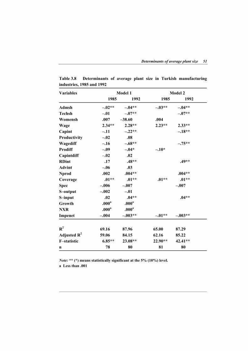
The regression results are shown in Table 3.8. In Model 1, all the explanatory variables are included. Insignificant variables are excluded in Model 2. The coefficient of determination, R2, is reasonably high for a cross-sectional regression and the F-statistic indicates that all models are statistically significant as a whole. None of the statistically significant coefficients have opposite signs for 1985 and 1992, i.e., results are consistent for 1985 and 1992. Since the regression model for 1992 seems to perform better, in terms of R2 and the number of statistically significant measures, we limit our discussion to that model.

The APS in Turkish manufacturing industries is positively correlated to the wage rate, R&D intensity, the number of products classified in the sector, the coverage ratio and the share of subcontracted inputs. It is negatively correlated to the share of administrative and technical personnel, capital intensity, intra-


sectoral wage differentials and the import penetration ratio. In other words, the share of SMEs will be large in industries in which:

1. the share of administrative and technical personnel is high, 2. the wage rate is low, 3. capital-intensive technology is used, 4. the intra-sectoral wage differential is large, 5. R&D intensity is low, 6. the scope for product differentiation is limited, 7. the coverage ratio is high, 8. the share of subcontracted inputs is low, and 9. the import penetration ratio is high. These results conform with our prior expectations. The only seemingly

unanticipated result is obtained for the capital intensity variable. The regression results for 1992 indicate that SMEs will have a higher employment share in capital intensive industries. This is, however, reasonable because, if all other relevant factors remain the same, a firm using labour intensive technology will employ more workers, i.e., it will be an LSE.

Our findings have major policy implications. The regression results point out the diversity of SMEs and the alternative strategies for survival. For example, it is found that the share of administrative and technical personnel has a positive impact on the share of SMEs (or a negative impact on APS). In other words, SMEs are competitive in those sectors in which skilled labour is essential. On the other hand, there are obstacles for the development of SMEs in R&D intensive sectors possibly because of their limited access to scientific knowledge. Moreover, high costs and the risks associated with R&D activities may inhibit SME activity. If this is the case, public policy should encourage SMEs to enter into technologically dynamic sectors by creating information networks and reducing their financial risk.


Table 3.8 Determinants of average plant size in Turkish manufacturing ndustries, 1985 and 1992 i

Variables Model 1 Model 2 1985 1992 1985 1992

Admsh –.02** –.04** –.03** –.04** Techsh –.01 –.07** –.07** Womensh .007 –38.60 .004 Wage 2.34** 2.28** 2.23** 2.33** Capint –.11 –.22** –.18** Productivity –.02 .08 Wagediff –.16 –.68** –.75** Prodiff –.09 –.04* –.10* Capintdiff –.02 .02 RDint .17 .48** .49** Advint –.06 .03 Nprod .002 .004** .004** Coverage .01** .01** .01** .01** Spec –.006 –.007 –.007 S–output –.002 –.01 S–input .02 .04** .04** Growth .000a .000a NXR .000a .000a I mpenet –.004 –.003** –.01** –.003** R2 69.16 87.96 65.00 87.29 Adjusted R2 59.06 84.15 62.16 85.22 F–statistic 6.85** 23.08** 22.90** 42.41** n 78 80 81 80 Note: ** (*) means statistically significant at the 5% (10%) level. a Less than .001

Chapter 4

Characteristics of small and medium-sized industry: A descriptive analysis 4.1 Method Small business economics explains the vitality of SMEs with two (contradictory) factors: On the one hand, small firms can compete with large firms, or complement their activities, on the basis of specialized competence in certain market niches. In this sense, small firms that have a more flexible structure can easily adapt themselves to a changing environment and market demand and continuously change the environment through innovative activities. This type of conceptualization highlights the dynamism of small firms. On the other hand, small firms become competitive and survive on the basis of low costs enjoyed in informal, disorganized markets. They may be less productive, but they can reduce their production costs utilising under-paid workers and, in many cases, owners and unpaid family members. The "flexible" work arrangements let large firms transfer the burden of risks and uncertainty to SMEs.

In this section, the characteristics of SMEs in Turkish manufacturing industries are described in detail. The aim is to present the picture of SMI in three different years: 1985, 1989, and 1992. The SIS conducted the Census of Industry and Business Establishments in 1985 and 1992. The Census covers all plants employing 10 or more people and a randomly selected group of plants employing

Characteristics of small industry 53

less than 10 people. The 1985 and 1992 data are used in our analysis to exploit the extended coverage of the Census data. The 1989 data are used as the mid-point of the 1985-1992 period. Moreover, as Şenses (1996: 9) mentioned, "[t]he 1989-93 period represented a sharp reversal of the trend in factor prices in the earlier [1980-1988] period and was characterized by a tendency of rising real wages, negative real rates of interest, and real appreciation of the exchange rate." The increase in real labour cost was almost 70 per cent from 1989 to 1992. Thus, the 1989 data are analyzed to discover the effects of changes in relative factor prices.

In the following sub-sections, the characteristics of SMEs are described in five categories: labour force, production structure, technological structure, capital and finance, and performance (Sections 4.2-4.6 respectively). A simple variance analysis is also performed to test if the differences among size groups are statistically significant. Unless otherwise indicated all data are taken from Güneş et al. (1996) with some minor modifications. Table 4.1 Number of 4-digit industries used in the variance analysis by stablishment size, 1985, 1989, and 1992 e

Plant size Private sector Public sector (employment) 1985 1989 1992 1985 1989 1992

Micro, <10 .. .. 78 a a a Small, 10-24 78 78 77 a a a Small, 25-49 78 76 74 9 9 13 Medium, 50-99 75 71 70 17 17 18 Large, 100-199 70 70 69 25 27 29 Large, 200-499 57 56 60 28 31 32 Large, 500+ 47 49 44 33 37 34 T otal (all groups) 405 400 472 112 121 126

a Plants in these groups are classified in the "Small, 25-49" group. .. means data are not available.

In our analysis, the measure under consideration is calculated for each establishment. The mean values for the establishments in each size group at the 4-


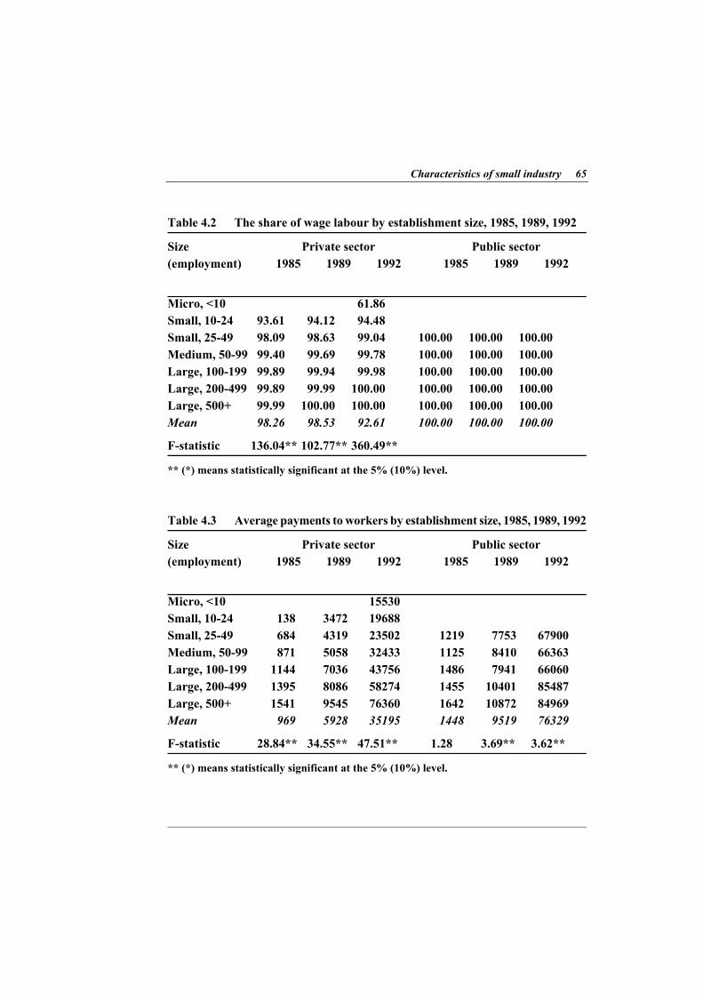
digit industry level are then calculated. The variance analysis among size groups is performed by using the data on the mean values. This method is used to eliminate inter-sectoral differences between SMEs and LSEs. The public and private sectors are analyzed separately. Since there are no establishments in some size groups in some sectors, the number of observations, i.e., the number of industries, is different among size groups. Table 4.1 shows the number of 4-digit industries by establishment size. 4.2 Labour force SMEs are conceived as owner-run establishments usually employing family labour. Table 4.2 reports the proportion of wage labour (paid employees) to total number of persons engaged including owners and unpaid family members. The public sector, by definition, does not employ any unpaid workers so that the share of employees is equal to 100% for all size groups. The data shows that the share of wage labour increases monotonically by size group and the difference among size groups is statistically significant in all years. Almost all persons engaged in private establishments employing more than 500 persons are wage earners. The share of owners and unpaid family members is very low in establishments employing more than 25 persons. It seems that micro establishments have a qualitatively different labour force in the sense that unpaid family labour has an important share.

Table 4.2 confirms the trend towards decline in non-wage labour in Turkish manufacturing industry, as discussed in Chapter 3. There is a gradual increase in the proportion of wage labour in all size groups. This is a rather interesting finding because it indicates a structural change affecting all establishments in all sectors. The decline in family labour could be as a result of the gradual elimination of traditional manufacturing activities.

Table 4.3 presents the data on average payments to employees by size groups. As may be expected, LSEs pay much higher wages* to their employees than SMEs. Average payments increase monotonically by size group and the difference among size groups is statistically significant. The ratio between the

* Payments to employees include all payments in the form of wages and salaries, overtime payments, bonuses, indemnities, payments in kind, per diems, gross income tax, social security, and pension fund premiums. It excludes social security, pension contributions, and the like payable by the employer.


average payments in large (500+ employees) and small (25-49) establishments was around 2.7 in the mid-1980s in the private sector. The wage disparity jumped to 3.9 in 1992 after the wage boom in the late 1980s and early 1990s. It is obvious that the organized labour in LSEs was able to benefit more than unorganized labour in this period.

It is interesting to observe wage differentials in the public sector in which the wage rate is expected to be independent of establishment size because of collective wage settlements. The differences in average payments among size groups in the public sector are statistically significant in 1989 and 1992. The wage differential, however, between large and small establishments is much lower in the public sector than in the private sector. Moreover, the wage disparity does not show any increase in the early 1990s in the public sector. The difference between average payments in large public and private establishments (500+ employees) seems to be negligible. However, small private establishments tend to pay lower wages than those paid in public establishments. This finding has important implications for the privatization policy pursued by the government.

The wage disparity in Turkey is large compared to developed countries. In Turkish private manufacturing industry, the average wage rate in plants with less than 25 employees is around 75% lower than the rate in plants with more than 500 employees. The corresponding wage disparity is around 25% in the US and 50% in Japan (Carlsson and Taymaz, 1994: 208).*

The wage differential between large and small firms can arise because of many factors. Firstly, as mentioned above, the labour employed in especially in the private SMEs is not usually organized. Secondly, the wage rate increases by seniority. Since LSEs tend to have longer terms of employment, they pay higher wages than SMEs. Thirdly, LSEs may have monopolistic power in their markets so that they can share a part of their excess profits with their employees. Finally,

* The wage disparity for the US and Japan is calculated for plants with less than 20 employees. In the UK, labour cost in plants with 500-999 and more than 1000 employees was 32% and 43% higher, respectively, than the labour cost in plants with 10-49 employees in 1984 (Bosworth, 1989: 61.)


the efficiency wage theory suggests that capital intensive technology users pay higher wages to eliminate risks associated with shirking and opportunistic behaviour. If LSEs use more capital-intensive technologies than their smaller counterparts, the wage rate will be higher in LSEs. Thus we expect differences in the composition of the labour force and the technological structure among size groups.

The share of the base wage* in average payments to employees displays a clear pattern in both the public and private sectors. Non-wage payments are not common in SMEs. The share of the base wage in payments is higher than 80% in small establishments and it declines monotonically by establishment size, and the inter-group differences are statistically significant in all years. The share of the base wage has increased after the late 1980s in both the public and private sectors. Non-wage payments have a much higher share in the public sector.

Tables 4.5 and 4.6 present data on the composition of the labour force by establishment size. The proportion of administrative employees has a clear pattern in the private sector. LSEs tend to employ more administrative employees than SMEs, and the difference is statistically significant. Micro establishments have a very low proportion of administrative employees. This fact proves that micro establishments do not have a refined specialization of labour. The proportion of administrative employees is higher in the public sector than in the private sector. However, there seems to be no difference among size groups in the public sector. Small public establishments employ proportionately as many administrative employees as do large public establishments.

There is not a significant difference between SMEs and LSEs in terms of the proportion of technical personnel (engineers and technicians). In 1985, private SMEs employ proportionately more technical personnel than LSEs but the difference is not statistically significant. There seems to be an increase in the proportion of technical personnel after 1989. Since firms tend to lay off unskilled workers in response to a general increase in wages, the increase in the proportion of technical personnel can partly be explained by the wage boom in the late 1980s.

* The base wage includes payments only in the form of wages and salaries, and excludes all other items explained in the footnote on p.53.


As in the case of other variables analyzed in this chapter, micro establishments arise as a distinct group. The share of technical personnel in much lower is micro establishments.

These findings show that the composition of the labour force in terms of administrative and technical personnel cannot explain the wage differential between SMEs and LSEs. We can conclude that these variables do not reflect skill differentials properly.

Table 4.7 presents data from a recent survey on the composition of the labour force and the average duration of employment in Turkish textile (ISIC 321 and 3222) and engineering (ISIC 38) industries. The distribution of employment by "production workers" and "administrative employees" is similar to the data presented in Tables 4.5 and 4.6. Table 4.7 reports the share of employees in R&D and design departments. The share of R&D and design personnel is higher in LSEs in both sectors. The average duration of employment tends to increase by establishment size, especially in the engineering industries. This result supports the argument that labour turnover decreases with plant size. More experienced, more stable and, therefore, well-paid workers are employed by larger plants.

Gender differences should also be studied in this context because recent studies suggest that female workers are paid less than male workers with the same qualifications because of labour market segmentation. Table 4.8 presents data on the proportion of female workers. There is a statistically significant difference among size groups in the private sector, but it seems that there is an inverted-U type relation between the share of women workers and the establishment size: small and large establishments employ proportionately less women workers than medium-sized establishments. This pattern is consistently maintained in all years. Thus, the employment of women workers cannot explain wage disparity in the private sector.

There is no difference among public establishments in terms of female employment. As in the case of other employment-related variables, the plant size is not an important factor in determining the gender composition of employment. Institutional regulations overrule any impact that the establishment size has on employment practices in the public sector. 4.3 Production structure This study aims to understand the factors that characterize SMEs in the Turkish

58 Small and medium-sized industry in Turkey manufacturing industry. Since the analysis is performed at an aggregate level, we do not examine the differences between SMEs and LSEs in specific sectors. We focus our attention rather on general characteristics of SMEs. Therefore, in this subsection, the share of value added in output, subcontracting practices, multi-shift work, and advertisement intensity will be examined.

Table 4.9 presents the data on the share of value added in output for different size categories. "Value added" is calculated as the difference between the values of output and input*, and is composed of factor payments (profits, returns to capital, and wage payments). The value added/output ratio is determined by three factors: i) the degree of vertical integration, ii) capital intensity, and iii) the extent of market power.

A vertically integrated establishment performs a large part of the activities necessary to produce the final product. Therefore, vertically integrated establishments have a higher value added/output ratio than those establishments specialized in certain activities. The value added/output ratio tends to increase with capital intensity in sectors producing bulk products (metalworking, etc.). On the other hand, in continuous process industries like petrochemicals, the value added ratio tends to decline because capital intensive technologies can transform inputs to outputs in very large volumes so that a high stock turnover ratio is achieved. The dominant firms in a market are able to raise the product price so that they earn excess profits. Therefore, ceteris paribus, oligopolistic firms will have a higher value added/output ratio.

As shown in Table 4.9, LSEs in the private sector tend to have a higher

* The value of output is calculated by subtracting the beginning of the year stock of finished and semi-finished goods from the total receipts from sales and services rendered to others, receipts from sales of transfers of electricity plus the end-of-year stock of finished and semi-finished goods, and the production value of the fixed assets produced by the establishment for own use. The value of input is calculated by subtracting the value of the end-of-year input stocks (raw materials, etc.) from the total value of goods and services purchased or transferred, electricity purchased and the beginning-of-year input stocks.

Characteristics of small industry 59 value added/output ratio than SMEs, and the difference has increased over time and has become statistically significant in 1989 and 1992. The mean ratio for all size groups has increased in both the public and private sectors although the difference between large and small establishments in the public sector is not significant. These results show all factors discussed above could be important in explaining differences between LSEs and SMEs.

Tables 4.10 and 4.11 presents the data on subcontracting practices. The share of subcontracted output is shown in Table 4.10. The subcontracted output share is used to measure the spread of receiving subcontracts. As may be expected, the subcontracted output ratio is much higher for SMEs in the private sector. Subcontracting has increased, mainly in the SME sector, after 1989. There is not a consistent pattern in the public sector, although the SMEs have a higher share of subcontracted output in 1992 in this sector also.

The share of subcontracted inputs in total inputs (Table 4.11) shows the degree of subcontracts offered by establishments. It is interesting to observe that LSEs do not use subcontracted input more than SMEs. On the contrary, SMEs relied on subcontractors to secure inputs more often than LSEs in 1985. No relationship is observed between establishment size and the share of subcontracted inputs in the public sector. These results show that the conventional view about SMEs supplying components and sub-assembly to large companies through subcontracting relationships is not correct. LSEs that have vertically integrated production do not offer subcontracts to other firms, whereas SMEs tend to offer subcontracts because of insufficient capacity and/or lack of technological capability. This finding is supported by micro-level studies. For example, Kaytaz found that "a large proportion of the subcontracting firms, both small and large, consider insufficient capacity as the main reason for offering subcontracts. ... Insufficient capacity being the main reason for offering subcontracts suggests that subcontracting practice in Turkey is temporary rather than developmental. This seems to be true particularly in textiles. In the small and medium-scale segment of the industry this reason in some cases overlaps with cost saving and lack of specific technology." (Kaytaz, 1994: 145, 147).

An important part of the production structure is related to shift work. Table 4.12 shows data on the share of second-shift in total hours worked. In all years, the share of second-shift work increases monotonically by plant size in the private sector. In other words, SMEs tend to work only one shift per day. The

60 Small and medium-sized industry in Turkey share of second-shift work in the public sector does not show any significant difference among size groups in 1985 and 1989. The reliance on second- and third-shift work in LSEs may be as a result of the need to use expensive machinery intensively. Moreover, LSEs can easily organize second-shift work thanks to their professional structures.

Since data on product characteristics is not available, we use advertisement intensity (the ratio of advertisement expenditure to sales revenue) as a proxy variable. We assume that advertisement intensity reflects the degree of product differentiation, because firms producing a wide range of differentiated products need to advertise heavily. If LSEs differentiate their products more than SMEs, than we expect a positive correlation between plant size and advertisement intensity.

Advertisement intensity is also related to the strategic behaviour of firms. An advertisement strategy can be used to raise entry barriers in oligopolistic markets. Therefore large firms that dominate their markets may use advertisement as an entry barrier to discourage potential firms from entering into their profitable markets.

Table 4.13 presents the data on advertisement activity. As expected, LSEs spend more on advertisement than SMEs in the private sector. The difference is statistically significant in all years. There is no significant difference in the public sector. It is also interesting to note that the public firms spend much less than the private firms. The advertisement intensity is seven times higher on average in the private than the public sector. 4.4 Technological structure As explained in Chapter 2, the recent debate on the role of SMEs emphasizes the flexibility of small firms in responding to a changing environment. The flexibility of SMEs can help them to overcome their (cost) disadvantages. It is argued that SMEs achieve flexibility by implementing flexible work arrangements and employing general purpose, flexible machinery and skilled workers. The debate on flexibility is usually based on a number of dichotomies: mass production vs flexible production, Fordism vs Toyotaism (or lean production), "Just-in-Case" vs "Just-in-Time" production, etc. Flexible firms will produce the product Just-in-Time, only when it is demanded. On the other hand, mass producers will build up work-in-process and finished goods inventories Just-in-Case, to avoid any


potential disruptions to supply and demand. Therefore we expect a negative correlation between the flexibility of production and the share of work-in-process and final product (output) stocks.

Table 4.14 shows the ratio between output stocks and total output (sales revenue). There seems to be no difference between SMEs and LSEs neither in the private nor in the public sector. There is no change in this ratio over time. The picture is similar for work-in-process inventories (see Table 4.15). The proportion of work-in-process stocks to output is around 1.5-2% in the private sector. SMEs kept less work-in-process stocks in 1992. The difference between SMEs and LSEs is statistically significant in 1992 when the micro establishments category is included. There is also no difference in the public sector. Thus, it is difficult to maintain the argument about the flexibility of SMEs in Turkish manufacturing industries.

Public establishments seem to keep more work-in-process and final product stocks than comparable private establishments. The mean ratios for work-in-process and final product stocks were around 1.2% and 5.5% respectively in the private sector in 1992. The corresponding figures for the public sector were around 6.6% and 12.8%. The cost of holding stocks can partly explain the difference in the performance of public and private firms.

The SIS conducted a detailed survey to collect data on machine stock in textile (ISIC 321 and ISIC 3222) and engineering industries (ISIC 38). The survey results, that are summarized in Tables 4.16 and 4.17, let us analyze the technological structure of SMEs (see Mintemur et al., 1996).

Table 4.16 presents the data on the composition of machine stock by age in the textile and engineering industries. SMEs have a younger machine stock than micro establishments and LSEs in both sectors. Thus, SMEs are more likely to use the best technology than other establishments. However, the data about the sources of machinery and equipment used in these sectors (Table 4.17) indicate the problems of SMEs in acquiring technology. Although SMEs use younger machines, LSEs prefer foreign machinery especially in the textile sector. The share of domestic machines in the stock of LSEs is around 50% in micro establishments and 34% in small establishments in the textile industry, and 71% in micro establishments and 61% in small establishments in the engineering industries. The share of domestic machines drops to 11% in the textile and 32% in the engineering industries.


SMEs utilize a significant amount of second-hand machinery because of financing problems. The share of second hand machinery in micro and small establishments is around 39% and 21%, respectively, in the textile industry, and 37% and 24% in the engineering industries. These results should be distressing for policy makers because they point out major problems for SMEs. The creation of domestic machine building capabilities seems to be a priority for policy makers who would like to promote the SME sector.

Finally, the depreciation allowances to output ratio is presented in Table 4.18. As expected, the ratio is higher for LSEs, i.e., LSEs use capital intensive technologies, because of two factor: i) LSEs substitute capital for labour because the wage rate is higher in LSEs. ii) The available technology is such that firms tend to use capital intensive technologies for higher output levels. Economies of scale through mechanization and automation may generate such a tendency.

Table 4.19 reports the data on R&D intensity. Since the Institute has collected the R&D data since 1992, the R&D intensity data are presented only for 1992. The data shows that R&D intensity is very low in all size groups (around 0.1%), and the difference among size groups is not statistically significant. 4.5 Capital and finance Financing the activities of SMEs and its effect upon capital structure have received considerable attention in policy discussions because it is frequently claimed, especially by the SME organizations, that SMEs usually lack the necessary financial resources and that they cannot gain access to low cost financing. Banks prefer to lend loans to established large firms that are considered to be less risky than SMEs.

Table 4.20 shows the equity/assets ratio (the inverse of the leverage multiplier) in Turkish manufacturing industries by plant size. There is not a clear relationship between the equity/assets ratio and establishment size. It seems that the equity/assets ratio was lower in small private establishments in 1985 and 1989, but it jumped to the mean value in 1992. A pattern is not observed in the public sector. The equity/assets ratio declined for all size groups after 1989 in the public sector, whereas it increased for all size groups except the largest establishments in the private sector.

The proportion of interest payments in sales revenue is shown in Table 4.21. It is interesting to observe that the interest cost is much higher in LSEs than

Characteristics of small industry 63 SMEs in the private sector. The proportion of interest payments to sales revenue is more than 10% in private LSEs whereas it is around only 5% in SMEs. It seems that SMEs do not borrow loans from the banking sector in the same volume as LSEs do. The SIS survey on SMEs in 1991 found that 53% of small establishments did not borrow any loan from the banking system, whereas the same figure is 38% in medium-sized establishments (SIS, 1994: 72).

The interest cost is invariant to establishment size in the public sector. However, the (mean) interest cost has increased rapidly in the public sector, from 5% in 1985 to 8% in 1989 and to 36% in 1992 as a result of the debt trap the public establishments have fallen in. 4.6 Performance The preceding analyses reveal that there are profound differences in the production and technological characteristics of SMEs and LSEs. There could be two factors that explain the differences between SMEs and LSEs. Firstly, they may arise as a result of rational decisions of owners/managers of establishments that operate in different economic environments. For example, an SME may adopt labour intensive technology because it could be the most profitable technology to produce at low volume under the current economic circumstances. If this is the case, the performance of an SME will be as good as that of an LSE, and the differences will not cause any concern for policy makers. Secondly, the differences can arise because of the disadvantages of being small. For example, SMEs may not have the capability to raise capital to finance their investment so that they are forced to adopt labour intensive technology even though it is not the most profitable alternative. If this is the case, the performance of SMEs will be worse than that of LSEs.

In this section, we compare the productivity and profit margin measures as performance criteria. The impact of establishment size on technical efficiency is analyzed in Chapter 5.

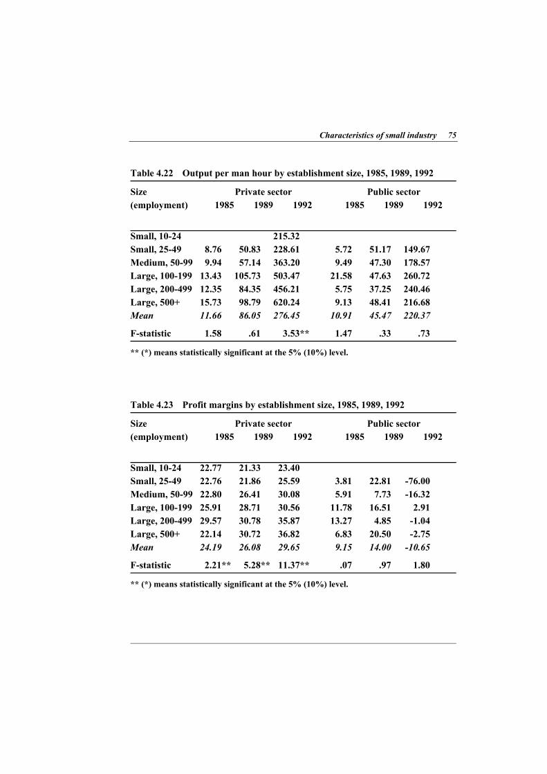
Table 4.22 presents the labour productivity data by establishment size. Productivity is measured as output per man hour at current prices. The level of productivity is much higher in LSEs than SMEs in the private sector. Establishments employing more than 500 persons were 200% more productive than small establishments in 1992. The order of magnitude of the productivity differential is roughly equal to the wage parity so that SMEs offset partially the

64 Small and medium-sized industry in Turkey adverse effects of low productivity by paying low wages.

LSEs in the public sector seem to have higher productivity than SMEs, but the difference is statistically insignificant and not consistent.

The second performance criterion we use in this section is the "profit margin" as defined by the proportion of value added minus wage cost to sales revenue (see Table 4.23). The profit margin is consistently higher in LSEs than in SMEs in the private sector. It increases monotonically by establishment size.

The profit margin grew in the late 1980s and early 1990s in almost all size groups, but the increase is higher in LSEs, i.e., LSEs have become more profitable in this period. As discussed in Section 4.2, the wage disparity increased after the wage boom in 1988-1989. The results confirm that the organized labour in LSEs were able to raise their wages, but LSEs were also able to increase their profits in spite of the wage boom.

Profit margins do not show any consistent pattern in the public sector. The mean value of the profit margin declined sharply in 1992, reflecting their disastrous financial situation.

The analyses in this section prove that SMEs in Turkish manufacturing industry have structural problems in competing with LSEs. Their productivity is low and they have to pay low wages and accept low profits to survive. These findings call for an active public policy to support SMEs.

Characteristics of small industry 65 T able 4.2 The share of wage labour by establishment size, 1985, 1989, 1992

Size Private sector Public sector (employment) 1985 1989 1992 1985 1989 1992

Micro, <10 61.86 Small, 10-24 93.61 94.12 94.48 Small, 25-49 98.09 98.63 99.04 100.00 100.00 100.00 Medium, 50-99 99.40 99.69 99.78 100.00 100.00 100.00 Large, 100-199 99.89 99.94 99.98 100.00 100.00 100.00 Large, 200-499 99.89 99.99 100.00 100.00 100.00 100.00 Large, 500+ 99.99 100.00 100.00 100.00 100.00 100.00 Mean 98.26 98.53 92.61 100.00 100.00 100.00

F -statistic 136.04** 102.77** 360.49**

** (*) means statistically significant at the 5% (10%) level. T able 4.3 Average payments to workers by establishment size, 1985, 1989, 1992


Micro, <10 15530 Small, 10-24 138 3472 19688 Small, 25-49 684 4319 23502 1219 7753 67900 Medium, 50-99 871 5058 32433 1125 8410 66363 Large, 100-199 1144 7036 43756 1486 7941 66060 Large, 200-499 1395 8086 58274 1455 10401 85487 Large, 500+ 1541 9545 76360 1642 10872 84969 Mean 969 5928 35195 1448 9519 76329

F -statistic 28.84** 34.55** 47.51** 1.28 3.69** 3.62**

** (*) means statistically significant at the 5% (10%) level.

66 Small and medium-sized industry in Turkey Table 4.4 The share of base wage in payments to employees by establishment ize, 1985, 1989, 1992 s



F -statistic 71.24** 109.67** 129.19** 1.98* 3.98** 4.79**

** (*) means statistically significant at the 5% (10%) level. Table 4.5 The proportion of administrative employees by establishment size,

985, 1989, 1992 1 Size Private sector Public sector (employment) 1985 1989 1992 1985 1989 1992


F -statistic 7.58** 3.38** 38.41** 1.31 1.13 1.06


Characteristics of small industry 67 Table 4.6 The proportion of technical personnel by establishment size, 1985,

989, 1992 1 Size Private sector Public sector (employment) 1985 1989 1992 1985 1989 1992


F -statistic 1.47 1.15 3.66** .67 .33 .38

** (*) means statistically significant at the 5% (10%) level. Table 4.7 The composition of labour force and the average duration of mployment in textile and engineering industries by establishment size, 1994 e

Size Production Administration R&D and design Duration (employment) Female Male Female Male Female Male of empl. (%) (%) (%) (%) (%) (%) (year)

Textile industry (ISIC 321 and 3222) Micro, <10 29.6 58.5 2.3 8.7 .3 .6 5 Small, 10-49 39.8 45.8 4.4 7.9 .9 1.3 4 Medium, 50-99 35.6 51.3 4.2 6.7 .9 1.4 4 Large, 100+ 35.0 53.1 2.4 6.6 1.8 1.1 7

Engineering industry (ISIC 38) Micro, <10 2.4 87.6 2.1 6.6 .3 1.0 5 Small, 10-49 7.5 75.8 4.4 10.2 .4 1.7 6 Medium, 50-99 7.6 73.7 4.3 10.7 .4 3.4 6 L arge, 100+ 9.2 70.4 3.5 13.3 .6 3.1 8

Source: Palas and Yıldırım, 1996.


Table 4.8 The proportion of women workers by establishment size, 1985, 1989, 992 1



F -statistic 2.71** 2.53** 4.35** .58 .39 .42

** (*) means statistically significant at the 5% (10%) level. T able 4.9 Value added/output ratio by establishment size, 1985, 1989, 1992



F -statistic 1.15 6.91** 10.11** .45 .27 .35


Characteristics of small industry 69 T able 4.10 Subcontracted output share by establishment size, 1985, 1989, 1992


Small, 25-49 3.57 4.37 5.36 .21 1.15 6.90 Medium, 50-99 3.23 2.59 3.18 1.70 4.59 5.73 Large, 100-199 2.56 2.42 3.41 .13 8.54 .23 Large, 200-499 .72 1.44 .93 .18 .29 .35 Large, 500+ 1.93 .77 .87 1.86 1.37 .96 Mean 2.54 2.50 2.99 .89 3.13 1.93

F -statistic 2.24* 4.11** 3.74** .63 1.60 2.21*

** (*) means statistically significant at the 5% (10%) level. T able 4.11 Subcontracted input share by establishment size, 1985, 1989, 1992


Small, 25-49 2.67 2.55 3.45 1.77 .50 .03 Medium, 50-99 2.53 2.01 2.70 .84 .07 1.73 Large, 100-199 2.28 2.04 2.58 .71 3.33 3.75 Large, 200-499 1.44 2.45 3.58 1.81 1.15 2.52 Large, 500+ .90 3.10 1.43 2.29 .80 2.56 Mean 2.09 2.39 2.84 1.55 1.33 2.44

F -statistic 2.96** .64 1.73 .28 1.29 .57



Table 4.12 The share of second-shift work in total hours worked by stablishment size, 1985, 1989, 1992 e


Micro, <10 .35 Small, 10-24 1.89 Small, 25-49 4.89 5.05 4.65 6.02 4.59 5.63 Medium, 50-99 7.69 7.38 6.62 18.73 16.82 16.43 Large, 100-199 11.09 11.42 12.79 13.21 17.80 12.68 Large, 200-499 21.14 16.73 18.91 14.08 19.70 22.04 Large, 500+ 23.40 23.09 24.69 17.72 19.55 21.21 Mean 12.35 11.73 8.65 15.01 17.70 17.17

F -statistic 31.41** 26.45** 64.19** 1.22 1.51 3.01**

** (*) means statistically significant at the 5% (10%) level. T able 4.13 Advertisement intensity by establishment size, 1985, 1989, 1992


Small, 25-49 .35 .44 .46 .09 .07 .32 Medium, 50-99 .42 .62 .50 .01 .07 .03 Large, 100-199 1.23 .64 .66 .04 .01 .25 Large, 200-499 1.04 .91 .93 .01 .04 .39 Large, 500+ .88 1.50 1.33 .02 .04 .55 Mean .75 .76 .72 .03 .04 .12

F -statistic 2.08* 2.62** 3.39** 2.07* .73 1.34


Characteristics of small industry 71 Table 4.14 The ratio between output stocks and total output by establishment ize, 1985, 1989, 1992 s



F -statistic .80 .72 1.26 .72 .95 .95

** (*) means statistically significant at the 5% (10%) level. Table 4.15 The ratio between work-in-process inventories and total output by stablishment size, 1985, 1989, 1992 e


Micro, <10 .23 Small, 10-24 1.17 1.35 .80 Small, 25-49 2.00 1.03 .93 6.42 2.31 6.51 Medium, 50-99 1.80 2.28 1.62 6.42 3.72 7.83 Large, 100-199 2.52 2.44 1.61 4.26 4.13 5.34 Large, 200-499 2.20 2.01 1.61 6.58 3.58 8.50 Large, 500+ 2.82 1.84 2.27 5.91 6.34 5.26 Mean 2.02 1.80 1.21 5.83 4.47 6.60

F -statistic 1.63 1.19 2.97** .19 1.15 .28



Table 4.16 The composition of machine stock by age in Turkish textile and engineering industries (%), 1995

Size (employment) Less than 10 years old 10 years and older

Textile industry (ISIC 321 and 3222) Micro, <10 63.74 36.26 Small, 10-49 74.41 25.59 Medium, 50-99 83.52 16.48 Large, 100+ 55.60 44.40

Engineering industries Micro, <10 48.67 51.33 Small, 10-49 53.35 46.65 Medium, 50-99 58.62 41.38 L arge, 100+ 41.22 58.78

Source: Mintemur et al., 1996. Table 4.17 The composition of machine stock by source in Turkish textile and engineering industries (%), 1995

Size (employment) Foreign Domestic New Second hand New Second hand

Textile industry Micro, <10 32.12 19.05 28.60 20.23 Small, 10-49 52.01 14.37 26.79 6.83 Medium, 50-99 63.16 12.36 22.74 1.74 Large, 100+ 80.57 8.44 10.24 0.74

Engineering industries Micro, <10 16.94 12.29 46.56 24.21 Small, 10-49 26.07 13.14 50.08 10.71 Medium, 50-99 29.72 17.06 46.69 6.53 Large, 100+ 61.36 6.78 28.77 3.09


Table 4.18 The ratio of depreciation allowances to output by establishment size, 985, 1989, 1992 1

Size Private sectora (employment) 1985 1989 1992

Micro, <10 0.79 Small, 10-24 1.86 3.65 2.81 Small, 25-49 3.90 3.62 3.28 Medium, 50-99 4.77 4.11 3.35 Large, 100-199 5.19 4.47 4.46 Large, 200-499 4.29 5.01 4.61 Large, 500+ 5.89 6.63 3.89 Mean 4.18 4.43 3.20

F -statistic 7.96** 2.22** 15.82**

** (*) means statistically significant at the 5% (10%) level. a The data on the public sector is not reported because of the lack of depreciation allowances data at the plant level. T able 4.19 R&D intensity by establishment size, 1992

Size Private sector Public sector (employment) 1992 1992

Small, 25-49 .10 .02 Medium, 50-99 .08 .01 Large, 100-199 .11 .22 Large, 200-499 .09 .11 Large, 500+ .11 .12 Mean .10 .11

F -statistic .22 .46



T able 4.20 Equity/assets ratio by establishment size, 1985, 1989, 1992


Small, 25-49 26.76 26.34 44.70 43.92 38.89 34.62 Medium, 50-99 39.15 40.67 45.67 34.04 40.65 19.87 Large, 100-199 24.72 39.15 43.77 39.22 32.10 30.29 Large, 200-499 40.57 41.26 43.00 46.66 43.81 28.80 Large, 500+ 37.09 47.55 42.38 40.38 45.57 28.21 Mean 35.20 38.11 44.07 41.01 40.93 28.30

F -statistic 3.61** 7.30** .32 .33 .55 .59

** (*) means statistically significant at the 5% (10%) level. Table 4.21 The proportion interest payments to sales revenue by establishment ize, 1985, 1989, 1992 s



F -statistic 10.9** 8.06** 14.2** 1.06 1.92 1.19



T able 4.22 Output per man hour by establishment size, 1985, 1989, 1992


Small, 10-24 215.32 Small, 25-49 8.76 50.83 228.61 5.72 51.17 149.67 Medium, 50-99 9.94 57.14 363.20 9.49 47.30 178.57 Large, 100-199 13.43 105.73 503.47 21.58 47.63 260.72 Large, 200-499 12.35 84.35 456.21 5.75 37.25 240.46 Large, 500+ 15.73 98.79 620.24 9.13 48.41 216.68 Mean 11.66 86.05 276.45 10.91 45.47 220.37

F -statistic 1.58 .61 3.53** 1.47 .33 .73

** (*) means statistically significant at the 5% (10%) level. T able 4.23 Profit margins by establishment size, 1985, 1989, 1992


Small, 10-24 22.77 21.33 23.40 Small, 25-49 22.76 21.86 25.59 3.81 22.81 -76.00 Medium, 50-99 22.80 26.41 30.08 5.91 7.73 -16.32 Large, 100-199 25.91 28.71 30.56 11.78 16.51 2.91 Large, 200-499 29.57 30.78 35.87 13.27 4.85 -1.04 Large, 500+ 22.14 30.72 36.82 6.83 20.50 -2.75 Mean 24.19 26.08 29.65 9.15 14.00 -10.65

F -statistic 2.21** 5.28** 11.37** .07 .97 1.80


Chapter 5

Technical efficiency, returns to scale and plant size 5.1 Returns to scale and technical efficiency There is an on-going debate on the relative (technical) performance of SMEs. In the preceding sections, it was found that small plants usually achieve lower productivity than larger plants and, consequently, tend to pay lower wages. In this section, we will analyze two possible factors behind productivity differentials: technical efficiency and returns to scale. Technical efficiency refers to the (efficient) use of existing resources. The technical efficiency level of a plant is measured as the ratio of its actual output level to the potential output that could be produced by the same inputs. In other words, a technically inefficient plant is, in principle, able to increase its output without any increase in inputs.

Returns to scale show the effects of a (percentage) change in all inputs on output. If there are constant returns to scale, the percentage change in output is equal to the percentage change in inputs. If there are increasing returns, the output increases more than inputs so that plants can increase their productivity by scaling up the production volume. For example, if the returns to scale parameter is equal to 1.2, a 1% increase in all inputs leads to 1.2% increase in output. The concept of returns to scale is closely related to the concept of economies of scale which demonstrates the relationship between production volume and unit production cost.

Technical efficiency, returns to scale and plant size 77

Large plants attain higher levels of productivity if there are increasing returns to scale, and/or if large plants are technically more efficient than small plants. Returns to scale are determined by production technology and production characteristics that are not controlled by the firm. The existence of strong returns to scale will favour high volume production and the creation of large establishments. Technical inefficiency at the plant level may arise because of differences in the technical knowledge, effort, etc., of individual plants. Technical inefficiency may also reflect differences in the vintage of production equipment (Torii, 1992). There is no intrinsic characteristic that make large plants more (or less) efficient. Large firms can increase their efficiency by securing access to specialized inputs (including knowledge), balancing their production processes, controlling demand fluctuations, etc. On the other hand, small firms may use their resources more efficiently thanks to their flexibility and superior incentive and monitoring mechanisms. Therefore the issue of relative efficiency of SMEs must be solved by empirical analysis.

In this section, the returns to scale and the effect of plant size on technical efficiency is estimated at the 4-digit industry level by using the stochastic production frontier approach. This approach explicitly takes into consideration the fact that some plants are technically inefficient. The stochastic production frontiers of all industries are estimated by using panel data of plants employing more than 25 people in the years 1987 to 1992. This method also enables us to estimate the rate and direction of technical change. The rate and direction of technical change for each industry are estimated by introducing time-dependent variables into the production function. Sector-specific factors including a "plant size" variable which influences the technical efficiency of manufacturing plants are also identified. Thus we also seek to find the relationship between average plant size and the rate of technical change to test the "Schumpeterian hypothesis" on the role of SMEs in the process of technical change as a prelude to Chapter 6 which focuses on the dynamics of new firms.


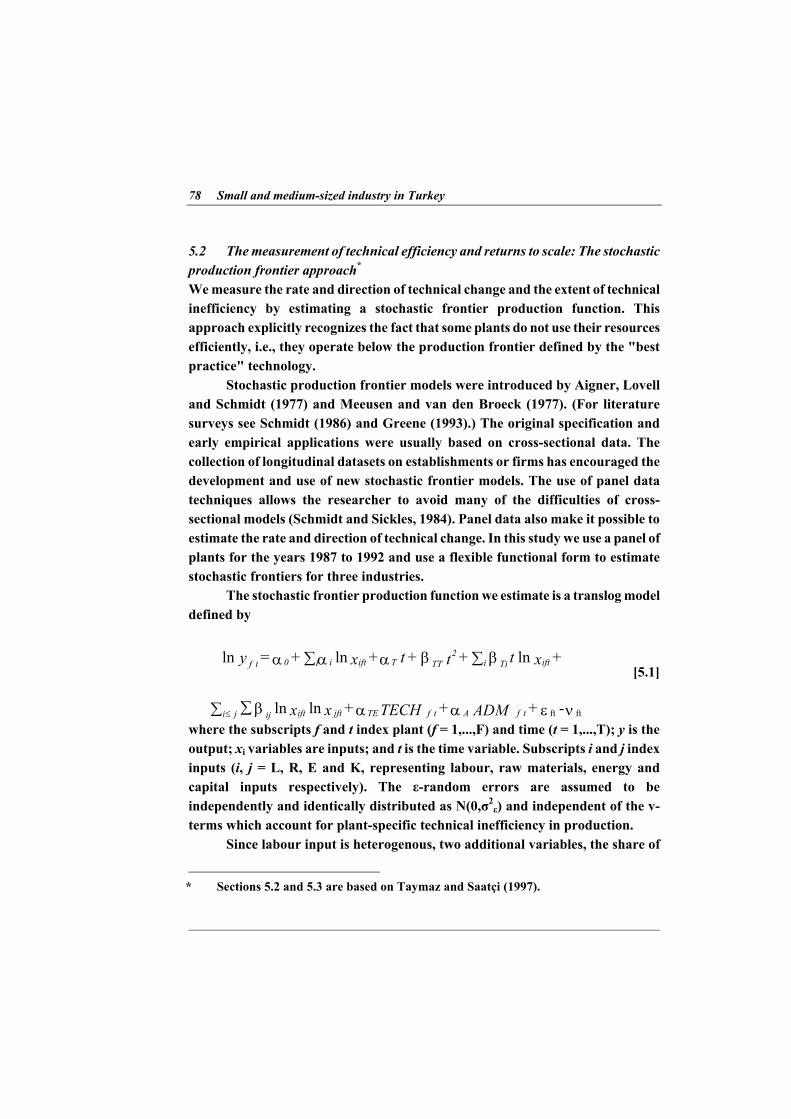
5.2 The measurement of technical efficiency and returns to scale: The stochastic production frontier approach* We measure the rate and direction of technical change and the extent of technical inefficiency by estimating a stochastic frontier production function. This approach explicitly recognizes the fact that some plants do not use their resources efficiently, i.e., they operate below the production frontier defined by the "best practice" technology.

Stochastic production frontier models were introduced by Aigner, Lovell and Schmidt (1977) and Meeusen and van den Broeck (1977). (For literature surveys see Schmidt (1986) and Greene (1993).) The original specification and early empirical applications were usually based on cross-sectional data. The collection of longitudinal datasets on establishments or firms has encouraged the development and use of new stochastic frontier models. The use of panel data techniques allows the researcher to avoid many of the difficulties of cross-sectional models (Schmidt and Sickles, 1984). Panel data also make it possible to estimate the rate and direction of technical change. In this study we use a panel of plants for the years 1987 to 1992 and use a flexible functional form to estimate stochastic frontiers for three industries.

The stochastic frontier production function we estimate is a translog model defined by

νεααβ

ββααα

ftft - lnln

lnlnln

+ ADM + TECH + x x

+ x t + t + t + x + = y

t f At f TEjftiftijj i

ifti2

iftit

∑∑

∑∑

≤

TiTTTi0f [5.1]

where the subscripts f and t index plant (f = 1,...,F) and time (t = 1,...,T); y is the output; xi variables are inputs; and t is the time variable. Subscripts i and j index inputs (i, j = L, R, E and K, representing labour, raw materials, energy and capital inputs respectively). The ε-random errors are assumed to be independently and identically distributed as N(0,σ2

ε) and independent of the v-terms which account for plant-specific technical inefficiency in production.

Since labour input is heterogenous, two additional variables, the share of

* Sections 5.2 and 5.3 are based on Taymaz and Saatçi (1997).


technical personnel (TECH) and the share of administrative personnel (ADM), are used as control variables. Note that the panel does not need to be balanced, i.e., data may not be available for some plants for some years.

The stochastic frontier model, as specified in Eq. 5.1, allows for non-neutral technical change. Technical change is input i using (saving) if βTi is positive (negative). Technical change is neutral if all βTis (βTL, βTR, βTE, and βTK) are equal to zero. The production function reduces to the Cobb-Douglas function with neutral technical change if all the βs are equal to zero.

The technical inefficiency effects, vft, are assumed to be independently distributed, such that vft is the non-negative truncation of the N(µft, σ2

v) distribution, where µft is defined by

z + = t f kk

m

=1 k0t f δδµ ∑

[5.2]

where zs are plant-specific factors that influence technical inefficiency. The z-variables which are involved in the inefficiency model are defined in Section 5.3 and are not functions of the x-variables in the frontier production function [5.1]. Hence the inefficiency model [5.2] specifies a neutral stochastic frontier, rather than the non-neutral model, proposed by Huang and Lui (1994).

The technical efficiency level of plant f at time t, EFFft, is defined as the ratio of the actual output to the potential output. Thus, EFFft is defined by

EFFft = . [5.3] e t f -ν

t + 2 + Tiiiijj ii j

iii x + = / = lnln∑≠

∂∂ xxE(y) βββαη lnln [5.4]

The elasticity of mean output with respect to the ith factor (input) is defined by (see Nishimizu and Page, 1982; Kumbhakar and Hjalmarsson, 1993)

The elasticity of scale (returns to scale), κ, is defined as i

κ The returns to scale are decreasing, constant or increasing if κ<1, κ=1, and κ>1, respectively.

. = iηΣ

. + t 2 + = t = RTP iTii

TTT ln∑∂∂ x E(y)/ lnln ββα [5.5]

The rate of technical progress (RTP) is defined by


Output elasticities and RTP are functions of the input levels. In the

estimation of Equation [5.1], the output and all the input variables are indexed around the sample geometric mean, i.e., arithmetic mean of the logged variable. Thus, one can easily calculate "average" output elasticities and RTP from Equations [5.4] and [5.5] since the logarithm of the geometric average of an input is equal to zero by definition.

Output (Q), like inputs, can be measured in physical or value terms. Since plants studied in this paper produce a number of products, we use an aggregated measure of output in value terms. Thus, the y-output is measured by total output (sales + increases in output stocks) at constant 1987 prices. Data about product types are not available for the period under consideration. For this reason, we do not include variables about product attributes in the model.

Four categories of inputs are used: capital (K), labour (L), energy (E), and raw materials (R). The "capital" input is defined theoretically as the services of capital goods in value terms. Since data for capital services and the replacement value of fixed assets are not available, we use a proxy variable. There were four alternatives: the number of machines installed, the total horsepower of installed equipment, depreciation allowances, and the book value of fixed assets. All these variables have well-known defects. In a previous version of this study (Taymaz and Saatçi, 1996), we estimated our models for all four capital variables to check if they led to significant differences in empirical results. "Physical" capital measures ("the number of machines" and "total horsepower of installed equipment") generate similar results. The same holds for "value" capital measures ("depreciation allowances" and "the book value of fixed assets"). Thus, we prefer to use the "depreciation allowances" variable because it is available for almost all plants. Moreover, "physical" measures are not meaningful especially for process industries.

The labour input (L) is measured as total number of hours worked in production. Energy (E) is measured as the value of fuel and electricity consumption at 1987 prices. The raw materials variable (R) is measured as the expenditure (at 1987 prices) on inputs (raw materials, supplementary materials, packaging materials, etc.) adjusted for stock changes. Since the labour input is heterogenous, two additional variables, the share of technical personnel (engineers and technicians) and the share of administrative personnel in total


employment, are used as control variables. The share of technical personnel (Tech) reflects the skill composition of production workers. If technical personnel are more productive than other employees, we expect a positive coefficient for this variable. The share of administrative personnel (Adm) is used to test their effects on output. 5.3 Efficiency effects variables The stochastic production frontier model includes the inefficiency term which is a linear function of some plant-specific factors. The following variables are used in the efficiency effects model in explaining the differences in the inefficiency levels of plants.

Region: "Region" is a variable whose value is defined by the proportion of the output of the region in which the plant is located relative to the total output. This variable is used to capture the effects of agglomeration and urbanization externalities. It is expected to have a negative coefficient in the inefficiency effects model (Equation 5.2) if the agglomeration and urbanization economies exist in the sector.*

Owned: "Owned" is a dummy variable which takes the value of 1 if the plant is individually owned.

Joint: This is another ownership dummy variable which takes the value of 1 if the firm is a joint stock company. The ownership variables (Owned and Joint) are used to test the effects of the legal status of companies on technical efficiency. These two variables compare the efficiency of individually owned firms and joint stock companies relative to other forms (limited liability companies, ordinary partnerships, etc.). In other words, the dummy variable for "other legal forms" is the omitted "legal status" variable.

Overtime: This variable is defined by the proportion of number of hours worked in the first shift to total number of hours worked. The Overtime variable is used to check the effects of shift-work on technical efficiency. A plant may improve technical efficiency by using its capital equipment in the second and third shifts. However, the efficiency of second and third shifts could be lower than the

* The negative sign of the coefficient of a variable shows that there is an inverse relationship between "technical inefficiency level" and the variable under consideration.


efficiency of the first (day-time) shift because of the negative impact of the unpleasant working times. If the first effect is dominant, the Overtime variable will have a negative coefficient.

S-input and S-output: The S-input and S-output variables are used to capture the effects of subcontracting relations. The "S-input" variable is measured as the proportion of inputs subcontracted to supplier firms to total (input) costs whereas the "S-output" variable is defined by the proportion of output subcontracted by other firms. This variable is equal to 1 if the firm is a "pure" subcontractor. Recent studies on small and mid-sized enterprises demonstrate the importance for the performance of firms of networking and close inter-firm relations. If networking in the form of subcontracting relations enhances technical efficiency, the coefficients of the S-input and S-output variables will have negative signs.

Adver: This variable shows the advertising intensity of the firm, and is defined as the share of advertisement expenditure in total costs.

Com: This variable measures the communication intensity of production and is defined as the share of expenditure on communications (PTT) services in total costs. The Adver and Com variables are included in the model to test the effects of product characteristics and strategic behaviour on technical efficiency. If these variables reflect the degree of product diversification, as we suggest, then we expect positive coefficients for these variables because diversified production consumes more resources. The Adver variable is not used for the cement industry because the industry spends almost nothing for advertisement.

Private and Foreign: These variables are defined by the proportion of shares held by private national and foreign agents, respectively. Private=1 if all shares of the company are held by (national) private agents. These variables are not used in the model of those industries that are mainly composed of private firms. The Private and Foreign variables, when they are included into the model, measure the efficiency of the private and foreign firms relative to the public firms.

Intel: "Intel" is a dummy variable which takes the value 1 if the firm received (purchased) any international technology through licensing, know how agreements, etc. The Intel variable is used to examine the effect of the source of technology. If the technology adopted through international technology transfer is superior to the domestic technology, those firms which acquired international technology will be more efficient. Hence, we expect a negative coefficient for the


Intel variable. Lsize: The Lsize variable is used to test if the size of a plant (measured in

terms of the log number of hours worked) affects its technical efficiency. A negative coefficient will support the hypothesis that large plants are more efficient than small plants.

Year dummies: Five year dummies (from 1988 to 1992) are included into the inefficiency effects model to capture changes in average efficiency levels. Year 1987 is the omitted time dummy.

5.4 Returns to scale in Turkish manufacturing Table 5.1 summarizes the average rate of technical change, returns to scale and efficiency at the 2-digit level. These variables are calculated from the estimated parameters of the stochastic production frontiers for all 4-digit industries. The FRONTIER 4.1 program written by Coelli (1992 and 1994) is used to obtain the estimates of the parameters of stochastic production frontiers. Table 5.2 shows correlations between variables under consideration.

Table 5.1 reveals that the rate of technical change is quite high in the engineering and wood products industries (4.8% and 4.3% respectively). The traditional industries like textiles, glass and cement have quite low rates of technical change (1.3% and 1.4% respectively). Table 5.3 presents "technical change" data at the 4-digit level. It is found that the office, computing and accounting machinery sector (ISIC 3825) achieves the highest rate of technical progress (35.1%). Although this sector is one of the leading high-tech sectors in developed countries, the rate of technical change is so high that it requires cautious interpretation. The cutlery and hand tools (10.8%), motor cycles and bicycles (9.9%), other chemical products (9.4%), sugar (8.4%), malt liquors and malt (8.3%), and basic chemicals (8.0%) industries enjoy high rates of technical progress. More than half of the 73 industries whose data allow us to estimate stochastic production frontiers achieve positive rates of technical change whereas technical regression is observed in nine industries. Low, and even negative, rates of technical change found in the traditional export industries like knitting and wearing apparel indicate that the competitive power of these industries is mainly based on low labour cost that is not sustainable in the long run. A special study focused on these industries is necessary to understand the specific aspects of the process of technical change.


The bias of technical change is also estimated at the average input use level. In 19 industries, labour using technical change is observed whereas labour saving technical change is found in only two sectors: sawmills and planing and electrical appliances. This result may not be surprising given the low level of wages in Turkey. On the input side, input saving change seems to dominate input using change: 17 industries adopt input saving technologies whereas input using technologies diffuse in only four industries. There is not a clear pattern observed for energy and capital inputs. Energy using (saving) technical change is observed in 10 (four) industries. The technology is capital saving in eight industries and capital using in three.

Estimated values of the returns to scale parameter for each 4-digit industry are shown in Table 5.4. The table also includes the data on average efficiency and average plant size in 1985. Increasing returns to scale are found in 25 industries whereas there are decreasing returns in only five (sugar, animal feeds, carpets and rugs, basic chemicals and ship building) industries. In other words, large scale production raises productivity and thus lowers unit production costs in 25 industries. Large plants have an apparent scale advantage in many industries. We can conclude that increasing returns to scale should be taken into consideration in explaining the productivity differentials between small and large plants.

Correlations between (the log value of) average plant size, the rate of technical change, the degree of returns to scale and average efficiency are shown in Table 5.2.* Average plant size, measured as the average number of employees per plant, is positively and significantly correlated to the rate of technical change. In other words, the rate of technical change is higher in industries populated with large plants. Although the correlation coefficient does not prove anything about the causality between the two variables, it could be argued that there is bi-directional causality between average plant size and the rate of technical change. On the one hand, large plants have the capability to perform R&D activities and to adopt new technologies so that they achieve a high rate of technical change. On the other hand, firms tend to grow faster in technologically dynamic industries.

Returns to scale are negatively correlated to average plant size but the

* Three outlier industries (office, computing and accounting machinery, radio, television and communication equipment, and other professional equipment industries) are excluded.


correlation coefficient is statistically significant only at the 10% level. Returns to scale tend to be lower (higher) when the average plant size is higher (lower). This result may indicate that the average plant size is above the "optimal" size in some industries.

Returns to scale are positively and significantly correlated with the average efficiency variable. This shows that plants are more efficient in those industries characterized by increasing returns to scale. In these industries, short run productivity increases are secured by expanding output. 5.5 The effect of plant size on technical efficiency The stochastic production frontier approach allows us to determine plant-specific factors that influence technical efficiency. As explained in Section 5.3, a number of variables are included into the efficiency effects model to test their effect on technical efficiency. The Lsize variable (the log number of hours worked) is used to test the effect of plant size on technical efficiency.

The Lsize variable is used for 66 industries. Table 5.5 shows the coefficient of the Lsize variable and its t-statistic for all industries.* (The results for other variables are not reported since they are not a major concern for this study. Detailed estimation results will be published separately.) The effect of plant size is summarized at the 2-digit level in Table 5.6.

Our findings reveal that in exactly half of the industries the plant size variable has a positive effect on the level of technical efficiency, i.e., large plants are more efficient than small plants in 33 industries. Small plants are more efficient only in the fruits and vegetables, tobacco, photographic and optical goods, jewellery, and other manufacturing industries.

Figures 5.1-5.4 depict the relationship between plant size (the log value of the number of hours worked) and technical efficiency in the wearing apparel, iron

* Because of the specification of the model (see Equation 5.1), a negative coefficient shows that there is a negative correlation with the Lsize variable and the level of inefficiency. In other words, a negative coefficient shows that large plants are, on average, technically more efficient than small plants.


and steel, motor vehicles, and jewellery industries, respectively. The positive correlation between plant size and technical efficiency is clearly seen in first three industries. Similar figures are observed for almost all other industries in which large plants are found to be more efficient.

Figures 5.1-5.3 reveal the fact that, although the average efficiency of small plants is lower, there are many small plants that are at least as efficient as large plants. In some industries, the most efficient plants are indeed small plants. The average efficiency level of small plants is lower mainly because there is more variation in the efficiency levels of small plants than in large plants. Although it is beyond the scope of this study, it is necessary to comment on this finding. As mentioned before, there is no intrinsic plant characteristics that explain why small plants should be less efficient. Our finding (low efficiency of small plants because of high variation in efficiency levels) is in accordance with the fact that business failure rates and turnover are higher for small than for large firms (see Caves and Barton, 1990: 118). New entrants to an industry are usually small plants, some of which are quite inefficient. The inefficient plants are closed quite rapidly while the efficient plants tend to grow. Therefore, the positive relationship between plant size and technical efficiency may simply reflect the effects of entry and selection processes.

To test the effects of the Lsize variable on the entry and selection processes, the correlation between the coefficient of the Lsize variable and the entry/selection rate is calculated. The entry/selection rate is defined as the proportion of workers in new (opened after 1985) and closed (in the 1985-92 period) plants to total number of workers in 1985 and in 1992. There is a negative and significant correlation between the entry/selection rate and the Lsize variable. In other words, the entry/selection rate is lower in those industries in which small plants, on average, are less efficient than large plants. The dynamics of new plants is analyzed in detail in Section 6.

As may be expected, the Lsize variable is negatively correlated to the average plant size. The higher the efficiency advantages of large plants over small plants, the higher the average plant size. The returns to scale variable is positively correlated to the Lsize variable: large plants tend to be more efficient than small plants if there are increasing returns to scale.

Our results show that there are significant increasing returns to scale in more than half of the manufacturing industries. A positive effect of plant size on

Date post:	04-Feb-2020
Category:	Documents
Upload:	others
View:	10 times
Download:	0 times

36 Small and medium-sized industry in Turkey40 Small and medium-sized industry in Turkey T able 3.5...

Documents