36 Spatial Prediction for Multivariate Non-Gaussian Data

36

Spatial Prediction for Multivariate Non-Gaussian Data

XUTONG LIU, ebay IncFENG CHEN, University at Albany, SUNYYEN-CHENG LU and CHANG-TIEN LU, Virginia Tech

With the ever increasing volume of geo-referenced datasets, there is a real need for better statistical esti-mation and prediction techniques for spatial analysis. Most existing approaches focus on predicting multi-variate Gaussian spatial processes, but as the data may consist of non-Gaussian (or mixed type) variables,this creates two challenges: (1) how to accurately capture the dependencies among different data types, bothGaussian and non-Gaussian; and (2) how to efficiently predict multivariate non-Gaussian spatial processes.In this article, we propose a generic approach for predicting multiple response variables of mixed types. Theproposed approach accurately captures cross-spatial dependencies among response variables and reducesthe computational burden by projecting the spatial process to a lower dimensional space with knot-basedtechniques. Efficient approximations are provided to estimate posterior marginals of latent variables for thepredictive process, and extensive experimental evaluations based on both simulation and real-life datasetsare provided to demonstrate the effectiveness and efficiency of this new approach.

CCS Concepts: � Machine Learning → Learning in probabilistic graphical models; SupervisedLearning by regression; � Probability and statistics → Probabilistic inference problems;

Additional Key Words and Phrases: Approximate bayesian inference, computational statistics, Gaussian andnon-Gaussian processes, geostatistics, Laplace approximation, predictive process model

ACM Reference Format:Xutong Liu, Feng Chen, Yen-Cheng Lu, and Chang-tien Lu. 2017. Spatial prediction for multivariate non-Gaussian data. ACM Trans. Knowl. Discov. Data 11, 3, Article 36 (March 2017), 27 pages.DOI: http://dx.doi.org/10.1145/3022669

1. INTRODUCTION

Increasing public sensitivity and concern regarding environmental issues have led tohuge amounts of spatial data being collected, and this volume continues to increase atan even faster pace. As one of today’s major research issues, the prediction of multi-variate spatial observations has attracted significant attention from many researchers,particularly those working in areas such as biology [McBratney et al. 2005], epidemi-ology [Kibria et al. 2002], geography [Gelfand et al. 2004], and economics [Chica-Olmo2007]. For example, weather forecasting is an important area of investigation withserious implications for many aspects of human life.

Spatial prediction is the process of estimating values of a target quantity at unvis-ited locations, based on the observed measures at sampled ones. In the univariate case,spatial prediction has been well studied for different data types, including continuous

Authors’ addresses: X. Liu, One Bellevue Center, 411-108th Avenue NE, Suite 400, Bellevue, WA 98004;email: [email protected]; F. Chen, UAB 426, 1215 Western Ave, Albany, NY 12222; email: [email protected]; Y. Lu,295 E Evelyn Ave 301, Sunnyvale, CA 94086; email: [email protected]; C.T. Lu, 7054 Haycock Road, Room 310,Falls Church, VA 22043; email: [email protected] to make digital or hard copies of part or all of this work for personal or classroom use is grantedwithout fee provided that copies are not made or distributed for profit or commercial advantage and thatcopies show this notice on the first page or initial screen of a display along with the full citation. Copyrights forcomponents of this work owned by others than ACM must be honored. Abstracting with credit is permitted.To copy otherwise, to republish, to post on servers, to redistribute to lists, or to use any component of thiswork in other works requires prior specific permission and/or a fee. Permissions may be requested fromPublications Dept., ACM, Inc., 2 Penn Plaza, Suite 701, New York, NY 10121-0701 USA, fax +1 (212)869-0481, or [email protected]© 2017 ACM 1556-4681/2017/03-ART36 $15.00DOI: http://dx.doi.org/10.1145/3022669

ACM Transactions on Knowledge Discovery from Data, Vol. 11, No. 3, Article 36, Publication date: March 2017.

http://dx.doi.org/10.1145/3022669

http://dx.doi.org/10.1145/3022669

36:2 X. Liu et al.

[Cressie 1991; Wackernagel 2003; Zhuo et al. 2011; Torgo and Ohashi 2011], discrete[Oliveira 2000; Webster and Oliver 1990], and Poisson spatial processes [Wolpert andIckstadt 1997]. Recently, a number of methods have been proposed for processing largeunivariate spatial datasets of different types, including fixed rank kriging [Cressie andJohannesson 2008], the knot-based spatial process [Banerjee et al. 2008], and the inte-grated nested Laplace approximation (INLA)-based predictive process [Rue et al. 2009].In many cases, geo-referenced datasets are multivariate. Multivariate spatial analysisrefers to those situations wherein there is an explicit vector of responses at each spa-tial location of interest and focuses on capturing potential relationships among spatiallocations and multiple responses. The prediction of multivariate spatial processes atunsampled locations plays an important role when there are cross-spatial dependenciesbetween multiple response variables of interest and there is therefore a considerableliterature on the modeling and prediction of multivariate spatial processes [Cressie1991; Ohashi and Torgo 2012]. Most related works focus on multivariate Gaussian pro-cesses (GPs), the key component of which is the modeling of cross-covariance functionsbetween attributes at different spatial locations.

Multivariate spatial interpolation has attracted a great of research due to its use-fulness in a wide range of applications, such as monitoring environmental pollution,managing responses to natural disasters, and public health-related activities. Obser-vations are often of mixed types, including numerical, nominal, and count, each ofwhich contains interesting information. In geological studies, it is often desirable topredict related properties of different types, such as moisture content (numeric), gran-ularity (count), and coloration (categorical) for pedological data [Chagneau et al. 2010].These mixed type responses and cross-variable dependencies further complicate thespatial inference process. The prediction of multivariate non-Gaussian (or mixed type)data has been identified as one of the 10 most important challenges in data miningfor the next decade [Piatetsky-Shapiro et al. 2006]. Consider the example of weathermonitoring. Weather forecasts can benefit from the more accurate estimation of real-time precipitation amounts, storm surges, and flood warnings for the protection oflife and property, but this requires predictive models that can extract all the criticalinformation simultaneously. The general objective here is to learn more about the rela-tionships between response variables (flood warnings, chance of rain, and wind speed)and predictor variables (location, elevation, season, and plant areas). This is a typi-cal application of spatial prediction involving mixed type observations, which createsmultiple issues: Challenge 1) Modeling mixed type observations. What is the best wayto model non-Gaussian multivariate spatial data that is as analytically intractable asGaussian data in spatial prediction? For example, modeling the mixed-type responsevariables involved in weather forecasting, including precipitation amounts (numeric),flood warnings (binary: yes/no), and cloud levels (ordinal: mostly or partly cloudy).Challenge 2) Capturing correlations among dependent variables. Multivariate spatialanalysis potentially involves two confounded dimensions of dependencies—betweendifferent responses, and between different spatial locations. Among these multivariateresponse types, there exist statistical relationships that need capturing. For example,the effects of wind speed on cloud level, and the possibility of flooding caused by theprecipitation amounts. Such dependencies need integrating into the predictive modelto improve the final estimation. Challenge 3) Improving scalability and availability.When training the predictive model, large amounts of weather data across multiplelocations are being collected and estimating the forecast model thus involves expensivematrix decompositions whose computational complexity increases in cubic order withthe number of spatial locations, rendering the task infeasible for large spatial datasets.Challenge 4) Analytically intractable posterior inferences. As an additional challenge,the likelihood related to non-Gaussian observations yields a distribution that is


Spatial Prediction for Multivariate Non-Gaussian Data 36:3

nonstandard and analytically intractable by nature. Therefore, approximate methodsare needed for the particular likelihood function of multivariate mixed-type responses.

Traditional spatial models often assume the outcomes follow normal distributions,which is difficult to verify empirically and overly restrictive. Only a limited amount ofresearch has been proposed to support non-Gaussian multivariate spatial processes.Markov Chain Monte Carlo (MCMC) methods [Schmidt and Rodriguez 2011] are pop-ular ways for addressing problems that are analytically intractable [Bandyopadhyay2005; Ridgeway and Madigan 2002; Li et al. 2008; Zhang and Sheng 2004; Boleyand Grosskreutz 2008]. However, it becomes prohibitively expensive for large spatialdatasets . To the best of our knowledge, there is no previous work that addresses allthe above challenging problems. This article proposes a flexible hierarchical Bayesianframework that supports simultaneous modeling and prediction of mixed-type obser-vations. A joint distribution for multivariate spatial responses is specified indirectlythrough specific link functions and the complicated dependencies among them arecaptured by the“cross-covariances,” which are easily parameterized. Efficient approxi-mations are integrated to estimate the posterior marginals of latent variables. In orderto reduce the computational burden, we project the spatial process to a lower dimensionspace by utilizing knot-based techniques [Banerjee et al. 2008]. Our generic approachmodel can also be applied to several data mining problems, including spatial outlierdetection [Wu et al. 2009, 2010], spatial temporal outlier detection [Liu et al. 2011;Wu et al. 2008], spatial-temporal scan [Mohammadi et al. 2009], and spatial anomalycluster identification [Neill and Moore 2004]. The major contributions of this work canbe summarized as follows.

—Constructing novel multivariate non-Gaussian hierarchical framework. The spatialmodel is based on a hierarchical framework and designed to take account of mixedtype random variables. Specifically, the mixed-type attributes are mapped to latentnumerical random variables via corresponding link functions, such as the logit func-tion for binary attributes and the log function for count attributes.

—Capturing dependencies among mixed-type responses. The dependency among mixedtype attributes is mapped to the relationship between their latent variables using aconditional variance covariance matrix. This enables the complicated correlations tobe captured more easily by parameterizing them in an analytically tractable way.

—Modeling a multivariate non-Gaussian reduced-rank predictive process. The knot-based technique is utilized to model the predictive process as a reduced-rank spatialprocess, which projects the process realizations of the spatial model onto a lowerdimensional subspace. This projection significantly reduces the computational cost.

—Designing an enhanced statistical approximation. By integrating the link functionsinto spatial references, the likelihood models involved are no longer analyticallytractable. Gaussian approximation and iterative Laplace approximation (LA) canthen be utilized to make approximations to the posterior marginal of latent variablesfor the predictive processes.

—Conducting extensive experiments for performance evaluations. Theoretical analysisand extensive experiments on both simulations and real datasets have been con-ducted for this study. The results clearly demonstrated the superior performance ofthe proposed hierarchical mixed model compared to existing state-of-the art compar-ison approaches, with comparable prediction accuracy and computational efficiency.

The remainder of this article is organized as follows. Section 2 reviews related works.Section 3 presents a generic multivariate non-Gaussian model that can not only modelmixed-type data (Challenge 1), but also capture correlations among them (Challenge 2).This section also introduces the reduced rank spatial predictive process (Challenge 3).Section 4 proposes an approximate inference for multivariate spatial prediction to


36:4 X. Liu et al.

solve the issue of analytical intractable inference (Challenge 4). Experiments on bothsimulated and real datasets are presented in Section 5, and the article concludes witha summary of the research in Section 6.

2. RELATED WORK

This section summarizes the current status of research achievements on spatial ref-erences, including spatial multivariate prediction for numeric data, spatial temporalmultivariate prediction, and spatial multivariate prediction for mixed-Type Data.

Spatial Multivariate Analysis for Numeric Data. Most research works [Bailey andKrzanowski 2000; Wang and Wall 2003] on multivariate spatial analysis have focusedon capturing potential relationships among spatial locations and multiple responses.The book by Wackernagel [2003] and the review by Gelfand and Banerjee [2010] pro-vide comprehensive surveys of a wide range of different spatial Gaussian multivariatemodeling and prediction techniques. For example, cokriging [Goovaerts 1997] exploitsthe spatial dependencies within the variables as well as the cross-spatial dependen-cies. Bailey and Krzanowski [2000] proposed two approaches that are concerned withthe identification of linear components and identifying factors. Wang and Wall [2003]designed a generalized common spatial factor model in which the parameters are esti-mated using the Bayesian method and MCMC techniques, and Ren and Banerjee [2013]discussed how to capture associations among responses by reducing the dimensions ofboth the length of the response vectors and the very large number of spatial locations.Christensen and Amemiya [2001] developed a generalized shifted-factor model that al-lows asymmetric spatial dependencies, and then they [Christensen and Amemiya 2002]went on to propose a latent variable-based approach to fitting model and estimatingparameter. Bonilla et al. [2008] described multi-task learning based on a GP prior thathas inter-task dependencies. The model utilized a convariance function on multiplefeatures under the assumption of noise-free observations. Kanevski [2012] proposed ageneric non-linear multivariate modelling by using the best MTL (Multitask Learning)group. The model was based on the criterion of nonlinear predictability of each depen-dent variable by analyzing all possible models composed from the rest of the variables.Finally, Minozzo and Ferracuti [2012] provided some valid constructions of stationarystochastic processes that are capable of modeling multivariate skew-normal data.

Multivariate Spatial-Temporal Data Analysis. Various approaches have been pro-posed for analyzing multivariate space-time data. Calder [2007] introduced a Bayesianconvolution model that provides a descriptive parametrization of the cross-covariancestructure of space-time processes and dimension reduction features. Zhu et al. [2005]extended a multivariate space-only model to space–time data by utilizing an adjust-ment of the Monte Carlo Expectation-Maximization algorithm. Reich and Fuentes[2007] designed a new Bayesian multivariate spatial statistical framework that buildson the stick breaking prior to handling sudden changed data in time or space. Choiet al. [2009] introduced a Bayesian hierarchical framework wherein a linear model ofcoregionalization was developed to account for spatial and temporal dependency foreach observation as well as the correlations among them. Grzebyk and Wackernagel[1994] presented the Bilinear Model that is suitable for modeling a coregionalizationin space or along the time axis.

Spatial Multivariate Prediction for Mixed-Type Data. A number of related workshave focused on non-Gaussian multivariate domains. Wibrin et al. [2006] explored theBayesian Maximum Entropy (BME) approach in which both continuous and categori-cal values are considered using a “cross-covariance” function. Schmidt and Rodriguez[2011] proposed MCMC methods for modeling multivariate counts, while Chagneau



et al. proposed a hierarchical Bayesian model for the modeling of Gaussian, count,and ordinal variables, and designed MCMC methods using the Gibbs sampler withMetropolis–Hastings (M-H) steps. Minozzo and Fruttini [2004] proposed a model basedon a generalized linear mixed multivariate framework. By integrating Monte CarloExpectation-Maximization, Minozzo and Ferrari [2013] designed another hierarchicalmodel in which non-Gaussian variables of different kinds can be processed simultane-ously. However, most of these methods are unable to provide a flexible framework thatsupports multivariate mixed-type data inferences simultaneously, including binomial,count, nominal, ordinal, and numeric data types.

3. THEORETICAL BACKGROUND

This section introduces the exponential family, the framework for the knot-based spa-tial process and the approximation Bayesian inference using INLA.

3.1. The Exponential Family

Let Y (s) be a response variable at the location s ∈ D ⊂ R2. It is assumed that Y (s)follows an exponential family distribution with the probability density:

f (Y (s)|θ (s), τ ) = exp(

Y (s)θ (s) − a(θ (s))d(τ )

+ h(Y (s), τ ))

, (1)

where θ (s) and τ are the model parameters. θ (s) is related to the mean of the distributionthat varies by location, and τ is a dispersion parameter related to the variance of thedistribution. The functions h(y(s), τ ), a(θ (s)), and d(τ ) are known. Y (s) has mean andvariance

E(Y (s)) := μ(s) = a′(θ (s)), (2)

Var(Y (s)) := σ (s)2 = a′′(θ (s))d(τ ), (3)

where a′(θ (s)) and a′′(θ (s)) are the first and second derivatives of a(θ (s)). Many populardistributions belong to this family, including the Gaussian, exponential, Binomial,Poisson, gamma, Inverse Gaussian, Dirichlet, and Chi-Squared Beta distributions.

For example, the Binomial distribution B(n(s), π (s)) has the density

p(Y (s)) =(

n(s)Y (s)

)π (s)Y (s)(1 − π (s))n(s)−Y (s). (4)

Taking log, we can rewrite the density function as

log p(Y (s)) = Y (s) log(

π (s)1 − π (s)

)+ n(s) log(1 − π (s)) + log

(n(s)Y (s)

). (5)

This shows that θ (s) = log( π(s)1−π(s) ), a(θ (s)) = n(s) log(1 + exp θ (s)), and h(Y (s), τ ) =

log( n(s)Y (s) ), where the second term in the density function is rewritten as log(1 − π (s)) =

− log(1 + exp θ (s)).

3.2. Knot-Based Spatial Process Model

Estimation and prediction in spatial process models often involve a high computationalcomplexity, which is cubic order with the number of spatial locations. To facilitate thespatial process, Banerjee et al. [2008] proposed a knot-based spatial predictive modelto reduce the computational cost through lower dimensional process observations.

Let us define a numerical random field Y (s) on a domain D ⊆ R2, and letY = (Y (s1), . . . , Y (sn))′ be the n × 1 vector of observed responses, each of which is


36:6 X. Liu et al.

accompanied by a p × 1 vector of spatially referenced predictors, x(s). The associatedspatial regression model can be represented as

Y (s) = xT (s)β + ω(s) + ε(s). (6)

The spatial process ω(s) captures spatial correlations and is a GP with zero meanand a covariance function C(s, s′; θ ). Spatial prediction requires matrix factorizationsinvolving the dense n×ncovariance matrix that may become prohibitively expensive fora large n. Instead, knot-based models consider a fixed set of “knots” S∗ = (s∗

1, . . . , s∗n∗ )

with n∗ � n. The GP ω∗(s) yields an n∗-vector of realizations over the knots, thatis, ω∗ = (ω(s∗

1), . . . , ω(s∗n∗ ))′, which follows a GP{0, C(s∗

i , s∗j ; θ )}. Spatial estimation at a

generic site s is operated through

ω(s) = E{ω(s)|ω∗} = cT (s; θ )C∗−1(θ )ω∗, (7)

where c(s; θ ) = [C(s, s∗j ; θ )n∗

j=1]. As shown in Equation (2), the predictive process w(s)is derived from the parent process ω(s). The realizations of ω(s) are referred to as thepredictions that are conditional on a realization of ω∗(s). Replacing ω(s) in model (6)with ω(s), we obtain the predictive process model

Y (s) = xT (s)β + ω(s) + ε(s), (8)

where ω(s) is defined as a spatially varying linear transformation of ω∗. The dimensionreduction is reduced from the original n to n∗; thus, the spatial interpolation processinvolves only n∗ × n∗ matrices.

It is important to select an appropriate number of knots as well as their spatiallocations. This is related to the problem of spatial design. There are two popular knotsselection strategies. One is to draw a uniform grid to cover the study region and eachgrid is considered as a knot. Another is to place knots such that each covers a localdomain and the regions with dense data have more knots. In practice, it is feasible tovalidate models by using different numbers of knots and different choices of knots toobtain a reliable and robust configuration.

3.3. Approximate Bayesian Inference Using INLA

The INLA [Rue et al. 2009] is a computational approach that is proposed as an alter-native of the time-consuming MCMC method. It approximates the marginal posteriorsof latent variables

π (vi|Y ) =∫

π (vi|θ, Y )π (θ |Y )dθ. (9)

This approximation is an efficient combination of LAs to the full conditionals π (θ |Y )and π (vi|θ, Y ), and finally executes numerical integration routines by integrating outthe parameter θ .

The INLA approach consists of three main approximations to obtain the marginalposterior for each latent variable. The first step is to approximate the full posteriorπ (θ |Y ), which is executed using the LA

π (θ |Y ) ∝ π (v, θ, Y )πG(v|θ, Y )

∣∣v=v∗(θ). (10)

As shown above, we need to approximate the full conditional distribution of π (v|Y, θ ),which can be achieved by a multivariate Gaussian density πG(v|Y, θ ) [Rue and Held2005]. v∗(θ ) is the mode of the full conditional distribution of v for a given θ and can beestimated using πG(v|Y, θ ). The posterior π (θ |Y ) will be used later to integrate out theuncertainty with respect to θ when approximating π (vi|Y ).



The second step executes the LA of the full conditionals π (vi|θ, Y ) for specified θvalues. The density π (vi|θ, Y ) is approximated using the LA defined by

πLA(vi|θ, Y ) ∝ π (v, θ, Y )πG(v−i|vi, θ, Y )

∣∣v−i=v∗(vi ,θ), (11)

where πG(v−i|vi, θ, Y ) refers to the Gaussian approximation of π (v−i|vi, θ, Y ) that takesvi as a fixed value. v∗(vi, θ ) is the mode of π (v−i|vi, θ, Y ).

Finally, we can approximate the marginal posterior density of vi by combining thefull posteriors obtained in the previous steps. The approximation expression is shownas follows:

π (vi|Y ) ≈∑

k

π (vi|θk, Y )π(θk|Y )�k. (12)

It is a numerical summation on a representative set of θk, with the area weight, �k fork = 1, . . . , K. Note that a good choice of the set of θk is crucial to the accuracy of theabove numerical integration.

4. SPATIAL MULTIVARIATE NON-GAUSSIAN MODEL

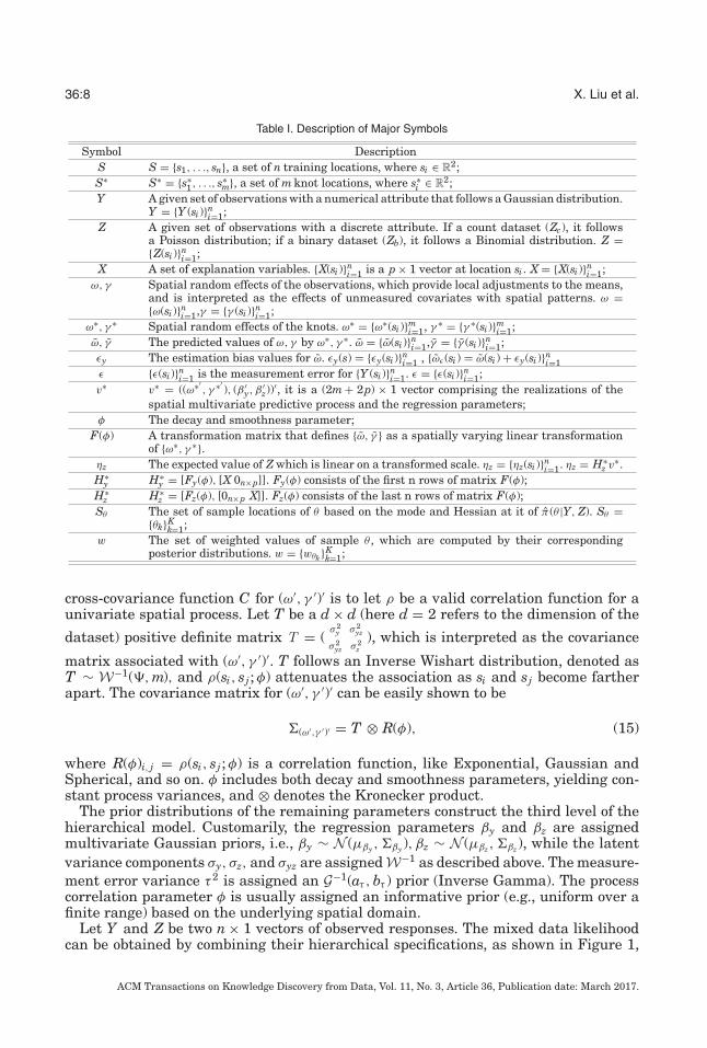
This section presents a spatial process model for random variables that is capableof dealing with Gaussian and non-Gaussian variables. The new multivariate modelproposed here is designed based on a Bayesian hierarchical framework that allowsany number of mixed-type response variables (Challenges 1 and 2). The computationalburden of modeling large mixed-type spatial datasets is addressed by integrating theknot-based predictive process (Challenge 3). Table I summarizes the key notations usedin this article.

4.1. Model Formulation

The spatial multivariate predictive model is specifically designed to deal with responsesof different types, which are assumed to follow an exponential family distribution. Here,we consider two different types: Gaussian and non-Gaussian variables (e.g., Poisson).

Let s1, . . . , sn be the n sampled locations, Y (si) be the Gaussian variable at locationsi, and Z(si) be the non-Gaussian variable, such as the Poisson variable. Let Y =(Y (s1), . . . , Y (sn))′ and Z = (Z(s1), . . . , Z(sn))′. Geostatistics typically assumes that theGaussian response variable Y (s) is modeled as a spatial regression model with a p × 1vector of spatially referenced predictors, x(s), such as

Y (s) = x(s)T βy + ω(s) + ε(s). (13)

The residual includes the spatial random effect, ω(s), and the independent processε(s), known as the measurement error. Usually, ε(s) ∼ N (0, τ 2). ω(s) provides a localadjustment to the mean, interpreted as the effect of unmeasured covariates on thespatial pattern.

Let the first stage of Z be the non-GP. Essentially, we assume that the function ofthe expected value of Z(si) is linear on a transformed scale, such as

ηz(s) ≡ g(E[Z(s)|θZ]) = x(s)T βz + γ (s), (14)

where g(·) is a suitable link function, and θZ is the parameter set of process Z(s).The Gaussian variable Y (si) and the non-Gaussian variable Z(si) depend on the

latent variables ω(si) and γ (si), respectively, which together are responsible for thespatial dependences. Given ω(si) and γ (si), the variables Y (si) and Z(si) are conditionallyindependent. The customary process specification for (ω′, γ ′)′ is a mean zero GP withcovariance function C, denoted as GP(0, C). The most obvious specification of a valid


36:8 X. Liu et al.

Table I. Description of Major Symbols

Symbol DescriptionS S = {s1, . . ., sn}, a set of n training locations, where si ∈ R

2;S∗ S∗ = {s∗

1, . . ., s∗m}, a set of m knot locations, where s∗

i ∈ R2;

Y A given set of observations with a numerical attribute that follows a Gaussian distribution.Y = {Y (si)}n

i=1;Z A given set of observations with a discrete attribute. If a count dataset (Zc), it follows

a Poisson distribution; if a binary dataset (Zb), it follows a Binomial distribution. Z ={Z(si)}n

i=1;X A set of explanation variables. {X(si)}n

i=1 is a p × 1 vector at location si . X = {X(si)}ni=1;

ω, γ Spatial random effects of the observations, which provide local adjustments to the means,and is interpreted as the effects of unmeasured covariates with spatial patterns. ω ={ω(si)}n

i=1,γ = {γ (si)}ni=1;

ω∗, γ ∗ Spatial random effects of the knots. ω∗ = {ω∗(si)}mi=1, γ ∗ = {γ ∗(si)}m

i=1;ω, γ The predicted values of ω, γ by ω∗, γ ∗. ω = {ω(si)}n

i=1,γ = {γ (si)}ni=1;

εy The estimation bias values for ω. εy(s) = {εy(si)}ni=1 , {ωε (si) = ω(si) + εy(si)}n

i=1ε {ε(si)}n

i=1 is the measurement error for {Y (si)}ni=1. ε = {ε(si)}n

i=1;v∗ v∗ = ((ω∗′

, γ ∗′), (β ′

y, β′z))

′, it is a (2m + 2p) × 1 vector comprising the realizations of thespatial multivariate predictive process and the regression parameters;

φ The decay and smoothness parameter;F(φ) A transformation matrix that defines {ω, γ } as a spatially varying linear transformation

of {ω∗, γ ∗}.ηz The expected value of Z which is linear on a transformed scale. ηz = {ηz(si)}n

i=1. ηz = H∗z v∗.

H∗y H∗

y = [Fy(φ), [X 0n×p]]. Fy(φ) consists of the first n rows of matrix F(φ);H∗

z H∗z = [Fz(φ), [0n×p X]]. Fz(φ) consists of the last n rows of matrix F(φ);

Sθ The set of sample locations of θ based on the mode and Hessian at it of π(θ |Y, Z). Sθ ={θk}K

k=1;w The set of weighted values of sample θ , which are computed by their corresponding

posterior distributions. w = {wθk}Kk=1;

cross-covariance function C for (ω′, γ ′)′ is to let ρ be a valid correlation function for aunivariate spatial process. Let T be a d × d (here d = 2 refers to the dimension of the

dataset) positive definite matrix T = (σ 2

y σ 2yz

σ 2yz σ 2

z), which is interpreted as the covariance

matrix associated with (ω′, γ ′)′. T follows an Inverse Wishart distribution, denoted asT ∼ W−1( , m), and ρ(si, sj ; φ) attenuates the association as si and sj become fartherapart. The covariance matrix for (ω′, γ ′)′ can be easily shown to be

�(ω′,γ ′)′ = T ⊗ R(φ), (15)

where R(φ)i, j = ρ(si, sj ; φ) is a correlation function, like Exponential, Gaussian andSpherical, and so on. φ includes both decay and smoothness parameters, yielding con-stant process variances, and ⊗ denotes the Kronecker product.

The prior distributions of the remaining parameters construct the third level of thehierarchical model. Customarily, the regression parameters βy and βz are assignedmultivariate Gaussian priors, i.e., βy ∼ N (μβy, �βy), βz ∼ N (μβz, �βz), while the latentvariance components σy, σz, and σyz are assigned W−1 as described above. The measure-ment error variance τ 2 is assigned an G−1(aτ , bτ ) prior (Inverse Gamma). The processcorrelation parameter φ is usually assigned an informative prior (e.g., uniform over afinite range) based on the underlying spatial domain.

Let Y and Z be two n × 1 vectors of observed responses. The mixed data likelihoodcan be obtained by combining their hierarchical specifications, as shown in Figure 1,



Fig. 1. Graphical model representation.

to derive a posterior distribution π (βy, βz, ω, γ, T , τ 2, φ|Y, Z) that is proportional to

π (φ) × G−1(τ 2|aτ , bτ ) × W−1(T | , m) × N((

ωγ

)|0, �(ω′,γ ′)′

)

×N (βy|μβy, �βy) ×n∏

i=1

N (Y (si)|x(si)T βy + ω(si), τ 2)

×N (βz|μβz, �βz) ×n∏

i=1

π (Z(si)|x(si)T βz + γ (si))). (16)

4.2. Reduced-Rank Spatial Multivariate Non-Gaussian Process

For the spatial multivariate non-GP model, both the estimation and prediction stepsrequire the (d ∗ n) × (d ∗ n) covariance matrix to be evaluated for the d dependentresponse variables. Unfortunately, fitting hierarchical mixed models often involves ex-pensive matrix decompositions whose computational cost is O((d∗ n)3), thus renderingsuch models not scalable for large spatial datasets. To facilitate the spatial process, aknot-based technique [Banerjee et al. 2008] can be utilized to reduce the computationalcost by lowering dimensional process, as this only requires a fixed set of “knots” overwhich spatial estimation is operated to be considered. In this section, the spatial mul-tivariate predictive model, referred to here as the reduced-rank spatial multivariatenon-GP, is constructed by projecting the full process into a subspace generated by aspecified set of representative locations. To generate the knots, a uniform grid is plottedacross the whole study region. Each grid is considered as a knot.

Consider a set of “knots,” S∗ = {s∗1, . . . , s∗

m}, representing the vector of correspondingcentroids of the m spatial clusters generated by the spatial attributes of the dataset.The latent variables (ω∗′

, γ ∗′)′ follow a mean zero Gaussian distribution with the co-

variance function C∗, denoted as GP(0, C∗). The covariance matrix for (ω∗′, γ ∗′

)′ is�(ω∗′

,γ ∗′ )′ = T ⊗ R∗(φ). R∗(φ) is the corresponding m × m covariance matrix, whereR∗(φ)i, j = ρ(s∗

i , s∗j ; φ)i, j=1,...,m. The spatial interpolant at a site s0 is estimated by(ω(s0)γ (s0)

)= E

{(ω(s0)γ (s0)

)∣∣∣∣(

ω∗γ ∗

)}= ϒ(s0)�−1

(ω∗′,γ ∗′ )′

(ω∗γ ∗

)

=(

f ωω (s0) f γ

ω (s0)f ωγ (s0) f γ

γ (s0)

)(ω∗γ ∗

). (17)

Here, ϒ(s0) = T ⊗ r(s0; φ)′, and r(s0; φ) is an m× 1 vector whose jth element is givenby ρ(s0, s∗

j ; φ). The f series represent four 1 × m matrices. This yields a spatial GP(ω′, γ ′)′ ∼ N (0, T ⊗ ρ), where ρ(si, sj ; φ) =ϒ(si)�−1

(ω∗′,γ ∗′ )′ϒ

′(sj), and (ω′, γ ′)′ is referred


36:10 X. Liu et al.

to as the predictive process derived from the parent process (ω′, γ ′)′. As shown inEquation (17), (ω(s)′, γ (s)′)′ is a spatially adaptive linear transformation of therealizations of (ω(s)′, γ (s)′)′ over S∗ with ϒ(s0)�−1

(ω∗′,γ ∗′ )′ comprising the coefficients of

the transformation.Replacing ω(s) and γ (s) in Equations (13) and (14) with ω and γ , we obtain the

reduced-rank predictive model,

Y (s) = x(s)T βy + ω(s) + ε(s), (18)

ηz(s) ≡ g(E[Z(s)|θZ]) = x(s)T βz + γ (s). (19)

Using Equations (38) and (39) as the likelihood, we derive a posterior distributionπ (βy, βz, ω

∗, γ ∗, T , τ 2, φ|Y, Z) that is proportional to

π (φ) × G−1(τ 2|aτ , bτ ) × W−1(T | , m) × N (βy|μβy, �βy) × N (βz|μβz, �βz)

× N((

ω∗γ ∗

)|0, �(ω∗′

,γ ∗′ )′

)×

n∏i=1

N (Y (si)|x(si)T βy + ω(si), τ 2)

×n∏

i=1

π (Z(si)|x(si)T βz + γ (si))). (20)

The reduced variability in ω often incurs an overestimation of the measurement er-ror variance τ 2. Banerjee et al. [2008] explained these biases. The predictive pro-cess systematically underestimates the variance of (ω′, γ ′)′ at any location s. It has0 ≤ var((ω′(s), γ (s)′)′|(ω∗′

(s), γ (s)∗′)′) = T −ϒ(s)�−1

(ω∗′,γ ∗′ )′ϒ

′(s), which denotes the bias un-derestimation over the observed locations. With regard to this issue, Finley et al. [2009]proposed replacing ω(s) and γ (s) in Equations (38) and (39) with ωε(s) = ω(s)+ εy(s) andγε(s) = γ (s) + εz(s). ( εy

εz) represents a process involving independent variables with spa-

tially adaptive variances. Using ωε(s) and γε(s) in place of ω(s) and γ (s) for the spatialprocess yields

π (φ) × G−1(τ 2|aτ , bτ ) × W−1(T | , m) × N (βy|μβy, �βy) × N (βz|μβz, �βz)

×N((

ω∗γ ∗

)|0, �(ω∗′

,γ ∗′ )′

)× N

((ωε

γε

)∣∣∣∣F(φ)(

ω∗γ ∗

), �(ε′

y,ε′z)′

)

×n∏

i=1

N (Y (si)|x(si)T βy + ωε(si), τ 2) ×n∏

i=1

π (Z(si)|x(si)T βz + γε(si))). (21)

F(φ) is a transformation matrix that defines {ω, γ } as a spatially varying lineartransformation of {ω∗, γ ∗}. According to Equation (17), ( ω(s0)

γ (s0) ) = ϒ(s0)�−1(ω∗′

,γ ∗′ )′(ω∗γ ∗ ) and

ϒ(s0) = T ⊗ r(s0; φ)′, and r(s0; φ) is an m × 1 vector whose jth element is given byρ(s0, s∗

j ; φ). Therefore, F(φ) = (T ⊗R(φ)′)�−1(ω∗′

,γ ∗′ )′ , where R(φ)′ is an n×mmatrix whoseith row is given by r(si; φ)′, and r(si; φ) is an m× 1 vector whose jth element is givenby ρ(si, s∗

j ; φ), for i = 1, . . . , n, j = 1, . . . , m. ( εyεz

) ∼ N (0, �(ε′y,ε

′z)′ ) and �(ε′

y,ε′z)′ is a 2n × 2n

matrix that consists of four diagonal matrices (n × n) in which the following four spec-ified diagonal elements ( (i, i)th (i + n, i)th

(i, i + n)th (i + n, i + n)th ) are computed as T − ϒ(si)�−1(ω∗′

,γ ∗′ )′ϒ′(si),

where ϒ(si) = T ⊗ r(si; φ)′. Finley et al. [2009] detailed the estimation of the modifiedpredictive process.



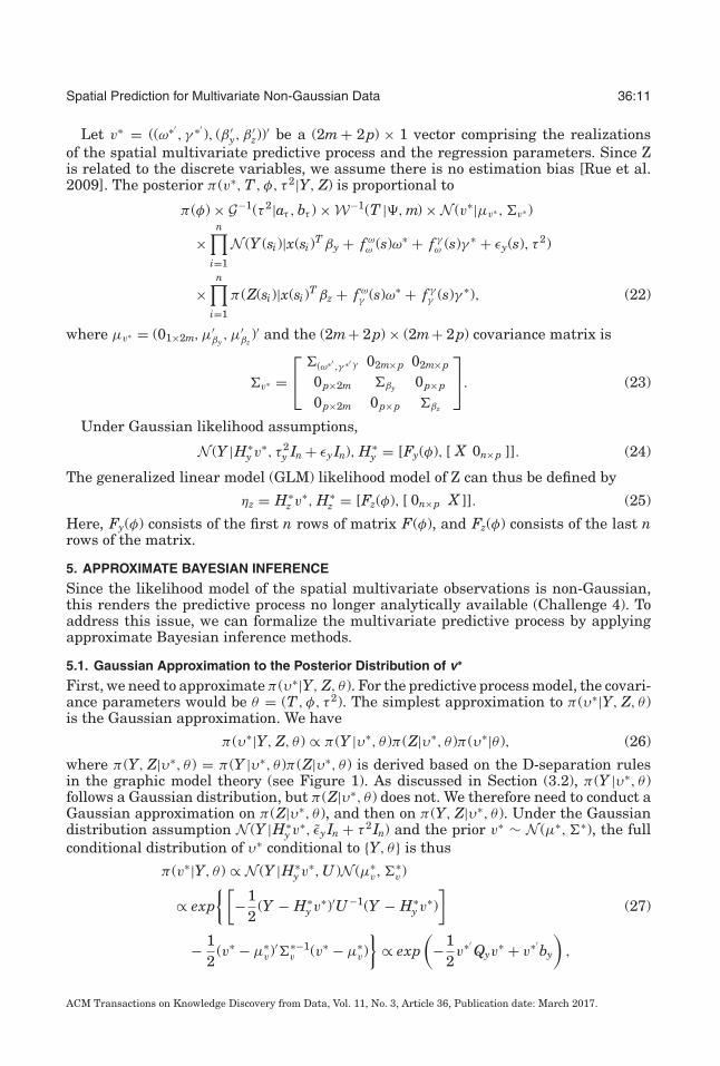
Let v∗ = ((ω∗′, γ ∗′

), (β ′y, β

′z))

′ be a (2m + 2p) × 1 vector comprising the realizationsof the spatial multivariate predictive process and the regression parameters. Since Zis related to the discrete variables, we assume there is no estimation bias [Rue et al.2009]. The posterior π (v∗, T , φ, τ 2|Y, Z) is proportional to

π (φ) × G−1(τ 2|aτ , bτ ) × W−1(T | , m) × N (v∗|μv∗ , �v∗ )

×n∏

i=1

N (Y (si)|x(si)T βy + f ωω (s)ω∗ + f γ

ω (s)γ ∗ + εy(s), τ 2)

×n∏

i=1

π (Z(si)|x(si)T βz + f ωγ (s)ω∗ + f γ

γ (s)γ ∗), (22)

where μv∗ = (01×2m, μ′βy

, μ′βz

)′ and the (2m+ 2p) × (2m+ 2p) covariance matrix is

�v∗ =⎡⎣ �(ω∗′

,γ ∗′ )′ 02m×p 02m×p

0p×2m �βy 0p×p

0p×2m 0p×p �βz

⎤⎦. (23)

Under Gaussian likelihood assumptions,

N (Y |H∗y v∗, τ 2

y In + εy In), H∗y = [Fy(φ), [ X 0n×p ]]. (24)

The generalized linear model (GLM) likelihood model of Z can thus be defined by

ηz = H∗z v∗, H∗

z = [Fz(φ), [ 0n×p X ]]. (25)

Here, Fy(φ) consists of the first n rows of matrix F(φ), and Fz(φ) consists of the last nrows of the matrix.

5. APPROXIMATE BAYESIAN INFERENCE

Since the likelihood model of the spatial multivariate observations is non-Gaussian,this renders the predictive process no longer analytically available (Challenge 4). Toaddress this issue, we can formalize the multivariate predictive process by applyingapproximate Bayesian inference methods.

5.1. Gaussian Approximation to the Posterior Distribution of v∗

First, we need to approximate π (υ∗|Y, Z, θ ). For the predictive process model, the covari-ance parameters would be θ = (T , φ, τ 2). The simplest approximation to π (υ∗|Y, Z, θ )is the Gaussian approximation. We have

π (υ∗|Y, Z, θ ) ∝ π (Y |υ∗, θ )π (Z|υ∗, θ )π (υ∗|θ ), (26)

where π (Y, Z|υ∗, θ ) = π (Y |υ∗, θ )π (Z|υ∗, θ ) is derived based on the D-separation rulesin the graphic model theory (see Figure 1). As discussed in Section (3.2), π (Y |υ∗, θ )follows a Gaussian distribution, but π (Z|υ∗, θ ) does not. We therefore need to conduct aGaussian approximation on π (Z|υ∗, θ ), and then on π (Y, Z|υ∗, θ ). Under the Gaussiandistribution assumption N (Y |H∗

y v∗, εy In + τ 2 In) and the prior v∗ ∼ N (μ∗, �∗), the fullconditional distribution of υ∗ conditional to {Y, θ} is thus

π (v∗|Y, θ ) ∝ N (Y |H∗y v∗,U )N (μ∗

v, �∗v )

∝ exp{ [

−12

(Y − H∗y v∗)′U−1(Y − H∗

y v∗)]

(27)

− 12

(v∗ − μ∗v)′�∗−1

v (v∗ − μ∗v)

}∝ exp

(−1

2v∗′

Qyv∗ + v∗′

by

),


36:12 X. Liu et al.

where U = εy In + τ 2 In, the full conditional precision matrix Qy = H∗′y U−1 H∗

y + �∗−1v ,

and the canonical parameter by = H∗′y U−1Y + �∗−1

v μ∗v.

The likelihood model of Z is non-Gaussian, so we need to expand the likelihood ina quadratic form utilizing the Gaussian approximation. The GLM likelihood of Z is∏

i π (Z(si)|ηz(si)), where the GLM parameter ηz = H∗z v∗ = [F(φz), [0n×pX]]v∗.

The distributions in a natural exponential family take the form

π (Z|ηz) = exp{ηzZ − f (ηz)}h(Z). (28)

For example, for a binomial distribution, Binomial(1, π ), ηz = log( π1−π

), f (ηz) = log(1 +exp(ηz)), and h(Z) = 1, while for the Poisson case, Poisson(λ), ηz = log(λ), f (ηz) = exp(ηz),and h(Z) = 1

Z! .By performing a Taylor expansion of f (ηz) = f (H∗

z v∗) to the second order, we obtainthe quadratic form of v∗,

π (Z|ηz) ∝ exp{−1

2v∗′

Qzv∗ + v∗′

bz

}, (29)

Qz = H∗′z ∇2 f (H∗

z v∗)H∗z ,

bz = H∗′z (Z − ∇ f (H∗

z v∗) + ∇2 f (H∗z v∗)H∗

z v∗).

Combining Equations (26), (27), and (29) gives

π (υ∗|Y, Z, θ ) ∝ exp[−1

2υ∗′

(Qy + Qz)υ∗ + υ∗′(by + bz)

]. (30)

Finally, the full conditional precision matrix Q = Qy + Qz, and the canonical parameterb = by + bz. Thus, the full conditional distribution is π (υ∗|Y, Z, θ ) ∼ N (Q−1b, Q−1). Wecan compute the required inverse and determinant of the size (2m+ 2p) × (2m+ 2p)matrix Qby utilizing the structure of H∗

z , H∗y , and �∗

v . Assuming m � p, the main cost ofthe matrix inversion is thus O(m3), since the number of knots is m. The supplementarymaterial provides further details of the Taylor expansion for the Binomial and Poissondistributions.

5.2. Laplace Approximation for the Posterior Distribution of θ

Unlike π (υ∗|Y, Z), the posterior π (θ |Y, Z) is usually highly skewed, and its approxima-tion as a Gaussian distribution is thus inappropriate [Rue et al. 2009]. The posteriorπ (θ |Y, Z) plays an important role in the inference of the marginal posterior of latentvariables. Taking υ∗ as an example, we can estimate the marginal posterior π (υ∗|Y, Z),which takes the form of

π (υ∗|Y, Z) =∫

π (v∗|Y, Z, θ )π (θ |Y, Z)dθ. (31)

It is possible to obtain a sample set {θ1, . . . , θK} from the input space of θ that rep-resents an approximate discrete form of the posterior p(θ |Y, Z). We can estimate theapproximate p(v∗|Y, Z) by

π (v∗|Y, Z) =K∑

k=1

π (v∗|Y, Z, θk)π (θk|Y, Z)wθk, (32)

where wθk is the weight of the sample point θk that can be measured by its normalizedprobability density. The critical step is to efficiently identify a representative sampleset {θ1, . . . , θK}, as well as the corresponding set of weights {wθ1, . . . , wθK}.



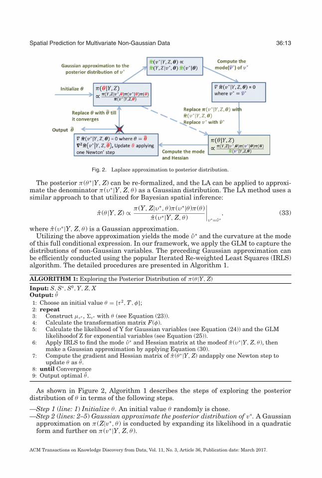
Fig. 2. Laplace approximation to posterior distribution.

The posterior π (θ∗|Y, Z) can be re-formalized, and the LA can be applied to approxi-mate the denominator π (υ∗|Y, Z, θ ) as a Gaussian distribution. The LA method uses asimilar approach to that utilized for Bayesian spatial inference:

π (θ |Y, Z) ∝ π (Y, Z|υ∗, θ )π (υ∗|θ )π (θ )π (υ∗|Y, Z, θ )

∣∣∣∣υ∗=υ∗

, (33)

where π (υ∗|Y, Z, θ ) is a Gaussian approximation.Utilizing the above approximation yields the mode υ∗ and the curvature at the mode

of this full conditional expression. In our framework, we apply the GLM to capture thedistributions of non-Gaussian variables. The preceding Gaussian approximation canbe efficiently conducted using the popular Iterated Re-weighted Least Squares (IRLS)algorithm. The detailed procedures are presented in Algorithm 1.

ALGORITHM 1: Exploring the Posterior Distribution of π (θ |Y, Z)

Input: S, S∗, S0, Y, Z, XOutput: θ

1: Choose an initial value θ = {τ 2, T , φ};2: repeat3: Construct μv∗ , �v∗ with θ (see Equation (23)).4: Calculate the transformation matrix F(φ).5: Calculate the likelihood of Y for Gaussian variables (see Equation (24)) and the GLM

likelihoodof Z for exponential variables (see Equation (25)).6: Apply IRLS to find the mode υ∗ and Hessian matrix at the modeof π (υ∗|Y, Z, θ ), then

make a Gaussian approximation by applying Equation (30).7: Compute the gradient and Hessian matrix of π (θ∗|Y, Z) andapply one Newton step to

update θ as θ .8: until Convergence9: Output optimal θ .

As shown in Figure 2, Algorithm 1 describes the steps of exploring the posteriordistribution of θ in terms of the following steps.

—Step 1 (line: 1) Initialize θ . An initial value θ randomly is chose.—Step 2 (lines: 2–5) Gaussian approximate the posterior distribution of v∗. A Gaussian

approximation on π (Z|v∗, θ ) is conducted by expanding its likelihood in a quadraticform and further on π (v∗|Y, Z, θ ).


36:14 X. Liu et al.

—Step 3 (line: 6) Update π (θ |Y, Z). The mode of v∗ as v∗ is calculated and π (θ |Y, Z) isupdated by replacing v∗ with v∗ as π (θ |Y, Z) ∝ π(Y,Z|υ∗,θ)π(υ∗|θ)π(θ)

π(υ∗|Y,Z,θ) .—Step 4 (line: 7) Update π (θ |Y, Z). The gradient and Hessian matrix of π (θ |Y, Z) are

computed and π (θ |Y, Z) ∝ π(Y,Z|υ∗,θ )π(υ∗|θ)π(θ )π (υ∗|Y,Z,θ)

is updated.—Step 5 (lines: 8–9) Output optimal θ . Steps 2–5 are repeated till the value of θ

converges. Finally, θ is output.

Among these steps, Step 3 has the highest time cost. Because the solution is analyticallyintractable, numerical optimization techniques need to be applied (see Appendix).

Computational Complexity: In Algorithm 1, suppose that l2 iterations are required tofind the mode v∗ and the Hessian matrix at the mode of π (υ∗|Y, Z, θ ), and the time costof Step 6 is O(l2 ∗ (n∗m2 +m3)). For Step 5, the Gaussian approximation of π (υ∗|Y, Z, θ )takes O(n ∗ m). Overall, Steps 2–8, which generate the converged gradient and theHessian matrix of π (θ |v∗), take O(l1 ∗ l2 ∗ (n ∗ m2 + m3) + l1 ∗ n ∗ m). Finally, samplingthe θ set and computing their corresponding weighted values take O(K). The overallframework is designed based on Newton’s method, whose convergence is generallyrapid. The performance on problems in R10,000 is thus similar to that on problems inR10, and the required number of Newton steps (l1) only increases modestly [Boyd andVandenberghe 2004]. Step 6 applies IRLS to capture the mode of π (υ∗|Y, Z, θ ), and inpractice five iterations (l2 = 5) are sufficient. Assuming m � K, m � l1, and m � l2,the total computational complexity of parameter estimation is therefore O(n ∗ m2).

5.3. Spatial Prediction via Laplace Approximation

Given a set of unsampled locations {s01 , . . . , s0

Nte}, we are interested in predicting the Y

and Z attribute values at these locations, denoted as Y 0 = (Y (s01 ), . . . , Y (s0

Nte))′ and Z0 =

(Z(s01 ), . . . , Z(s0

Nte))′. The first step is to estimate the posterior distributions of the corre-

sponding latent variables π (ω0|Y, Z) and π (γ 0|Y, Z), where ω0 = (ω(s01 ), . . . , ω(s0

Nte))′ and

γ 0 = (γ (s01 ), . . . , γ (s0

Nte))′. The posterior distributions of Y 0 and Z0 can then be obtained

as

π (Y 0|Y, Z) =∫

π (Y 0|ω0)π (ω0|Y, Z)dω0, (34)

π (Z0|Y, Z) =∫

π (Z0|γ 0)π (γ 0|Y, Z)dγ 0. (35)

We denote v0 = (ω0′, γ 0′)′. Given the approximated π (v∗|Y, Z, θ ) and π (θ |Y, Z) obtained

in Sections 4.1 and 4.2, the posterior distribution π (v0|Y, Z) can be estimated at eachθ sample by

π (v0|Y, Z, θ ) ≈ π (Y, Z|v0, v∗)π (v0, v∗|θ )π (v∗|v0, Y, Z, θ )

∣∣∣∣υ∗=υ∗

. (36)

Furthermore, it can be computed as

π (v0|Y, Z) ≈K∑

k=1

π (v0|Y, Z, θk)π (θk|Y, Z)wθk. (37)

Based on the above theoretical analysis, the main procedures involved in predictingmultivariate non-Gaussian variables are described by Algorithm 2. As shown in Fig-ure 3, Algorithm 2 introduces spatial prediction of multivariate non-Gaussian variablesvia LA as the following steps.



Fig. 3. Spatial prediction via Laplace approximation.

ALGORITHM 2: Spatial Multivariate Non-Gaussian Prediction

Input: S, S∗, S0, Y, Z, X, X0, θOutput: Y 0, Z0

1: Explore the contour of π(θ |Y, Z) based on its mode and Hessian matrix at the mode, obtainK sample locations, Sθ = {θ1, . . ., θK}.

2: Compute and normalize {π(θ1|Y, Z), . . ., π (θK|Y, Z)} to obtain the set of weightsw = {wθ1 , . . ., wθK } as wθk = πk(θk|Y,Z)∑K

k=1 πk(θk|Y,Z).

3: for k = 1 to K do4: Construct μv∗ , �v∗ with θk and S∗ (see Equation (23)).5: Calculate the transformation matrix F(φ) with θk, S∗, S, X.6: Calculate the likelihood of Y for Gaussian variables (see Equation (24)) and the GLM

likelihoodof Z for exponential ones (see Equation (25)).7: Calculate the mode, the Hessian matrix at the mode of π (υ∗|Y, Z, θk), and its Gaussian

approximation (see Equation (30)).8: Predict Y 0

k , Z0k for new locations S0. (see Equations (34) and (35))

9: end for10: Calculate the final Y 0, Z0 values as Y 0 = ∑K

k=1 Y 0k × wθk , Z0 = ∑K

k=1 Z0k × wθk

—Step 1 (line: 1) Generate sample set of Sθ . First, the contour of π (θ |Y, Z) is exploredbased on its mode and Hessian matrix at the mode, and then its K sample values aregenerated.

—Step 2 (line: 2) Compute the weighted set of ωθK . The weighted values of θ samplesare computed as wθk = πk(θk|Y,Z)∑K

k=1 πk(θk|Y,Z).

—Step 3 (lines: 3–9) Predict Y k0 and Zk

0 at each sample θk. Each θk(k = 1, . . . , K) is utilizedto perform a Gaussian approximation on the posterior distribution of v∗ and thenthe mode of π (υ∗|Y, Z, θ ) is calculated, which contributes to predict the multivariateobservations Y 0

k and Z0k .

—Step 4 (line: 10) Obtain the final predicted Y 0 and Z0. Finally, the predicted Y and Zare calculated as Y 0 = ∑K

k=1 Y 0k × wθk, Z0 = ∑K

k=1 Z0k × wθk.

Computational complexity: Step 6 dominates the computational costs here, becauseit is analytically intractable. With the numerical optimization discussed in Sections 4.1and 4.2, it takes O(n∗m) to operate a Gaussian approximation of π (υ∗|Y, Z, θk) for eachsample θk. Computing the mode and Hessian matrix for π (v∗|Y, Z, θk) costs O(l2∗(m3+n∗m2)). Repeating Steps 1–7 for K sample θs therefore takes O(K∗(n∗m+l2∗(m3+n∗m2))).


36:16 X. Liu et al.

Table II. Parameter Settings in Simulations

Variable Setting descriptionData type Gaussian(Y)+Binomial(Z), Gaussian(Y)+Poisson(Z), Binomial(Y)+Poisson(Z)Ntr, Nte Ntr = 1, 000, Nte = 400, 500. Training data were randomly generated at Ntr spatial

locations {si}Ntri=1 for the range [0,50]×[0,50] units. Test data were generated at Nte

spatial locations {si}Ntei=1 over the same range.

βy, βz The regression coefficient βy = [2, 2]′, βz = [2, 1]′ in G+P; βy = [0.5, 0.5]′, βz =[0.1, 0.1]′ in G+B; βy = [0.1, 0.1]′, βz = [2, 1]′ in B+G.

σy, σz, σyz σ 2y = 4, σ 2

z = 3.24, σ 2yz = 2.52 in all types of simulations.

φ φ = 25 in all types of simulations.τ The measurement error variance, τ2, was set to 1 in both G+B and G+P simulations.Correlationmodel

An exponential spatial correlation function C(h, φ) = σ 2exp(− hφ

) was used in all typesof simulations.

Fig. 4. Density maps of a typical G+B simulation.

The total computational complexity of the Spatial Multivariate Non-Gaussian Predic-tion algorithm is thus O(n ∗ m2), assuming m � K and m � l2.

6. EXPERIMENTAL RESULTS AND ANALYSIS

This section evaluates the effectiveness and efficiency of our proposed framework basedon experiments on simulations and four real-life datasets. We focus on three bivariatescenarios: (1) the response variables consist of one Gaussian and one binomial, G+B; (2)the response variables consist of one Gaussian and one Poisson, G+P; (3) the responsevariables consist of one binomial and one Poisson, B+P. All the experiments wereconducted on a PC with Intel(R) Core(TM) I5-2400, CPU 3.1GHz, and 8.00GB memory.The development tool was MATLAB 2011.

6.1. Simulation Study

6.1.1. Simulation Settings.Dataset: We utilized a similar simulation model in Chagneau et al. [2011]. The pa-

rameter settings used in our experiments are shown in Table II. We also evaluateddifferent combinations of parameters and observed similar patterns. Figure 4 depictsdensity maps of the numerical(Y) and binary(Z) responses from a typical G+B simu-lation, revealing the complicated distributions involved and clearly illustrating why ahigher processing ability is required for the predictive models.



Seven state-of-the-art competing methods: Based on our literature survey, there onlyexist two methods proposed for predicting multivariate non-Gaussian spatial data.One is the BME method by Wibrin et al. [2006] that only supports the mixture ofone numerical and one categorical value. Another method is the MCMC designed byChagneau et al. [2011] that is based on the Gibb sampler with M-H steps. We observedthat the BME method is only restricted to bivariate data with one Gaussian and oneCategorical, and MCMC method is flexible for a variety of mixture types. Hence, weimplemented the MCMC method using the same framework (Gibbs sampler with M-Hsteps) and denoted this method as Spa-Multi-MCMC.

We also implemented an R toolbox function named “MCMCglmm” using the sameMCMC framework, denoted as Multi-MCMC. Spa-Multi-MCMC and Multi-MCMC donot scale well to large datasets. Therefore, we designed two approximate versions ofthem, namely, Spa-Multi-MCMC-K and Multi-MCMC-K. CART (Classification and Re-gression Trees) [Breiman et al. 1984], MARS (Mulivariate Adaptive Regression Splines)[Friedman 1991], and Treenet (also known as MART, Multiple Additive RegressionTrees) [Friedman 2000] are popular techniques for non-spatial predictive modeling.They have been implemented into the Salford Systems [2017]. We used them to makepredictions for Y and Z separately. The model proposed in this article is identified asSpa-Multi-INLA.

Performance metric: We ran the experiments with 20 realizations of each parametercombination and then calculated the mean and standard deviation of every parametercombination in the multivariate process model. For each observation, we computedthe Mean Absolute Error (MAE) for numerical and count observations, and the predic-tion error for binary ones based on their corresponding predicted and true values. Tovalidate the new model’s effectiveness and efficiency, we compared the results of es-timations, predictions, and response times for the Spa-Multi-INLA and MCMC-basedapproaches, as well as CART, MARS, and Treenet. All parameters used in CART, MARS,and Treenet were tuned using cross-validation (10-folder), like the MinLeafSize, Tree-Size, and NumofTrees, and so on. For both simulation and real datasets, the corre-sponding parameters were selected by the optimal points given a visual representationof the cross-validation results in CART, MARS, and Treenet models. Finally, we utilizedMoran’s I-statistic to capture the spatial dependency of the numerical observations.

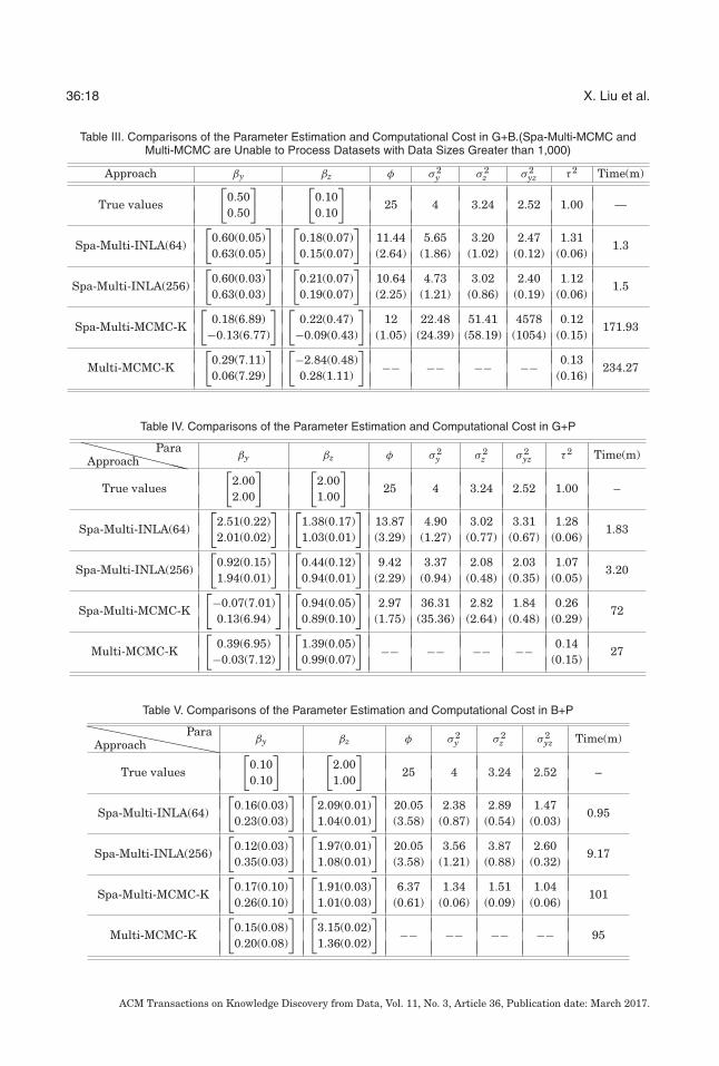
6.1.2. Simulation Results.Model parameter estimates: Tables III, IV, and V show the estimation results for the

model parameters for datasets of size 1,000 for the G+B, G+P, and B+P simulations,respectively. “Spa-Multi-INLA(64)” refers to our approach with a knot size equal to 64.No results are shown for Multi-MCMC and Spa-Multi-MCMC because they becamevery slow when the data size exceeded 1,000. The iterations of Spa-Multi-MCMC-Kand Multi-MCMC-K were set to 3,000 iterations, and K equal to 170 blocks (clusters).Also, there are no results for CART, MARS, and Treenet in these tables. This isbecause these models do not include these parameters. Instead, these ran on theSalford tool, which is a powerful well-developed and optimized tool, and it was notconsidered reasonable to directly compare their running times with those of the LAand MCMC-based approaches, both of which ran on Matlab. However, we did comparethe prediction performances of Y and Z among all of these approaches and the resultsare shown in Figure 5. By comparing the estimated parameters with true values, weobserved our method was able to accurately estimate most of the model parameterswith only small deviations compared to the other two MCMC-based methods for allsimulations. The true range parameter φ is 25, but both the LA- and MCMC-basedapproaches underestimated the range parameter at around 11. This indicates thedifficulty of capturing the degree of spatial autocorrelation over the spatial distance.


36:18 X. Liu et al.

Table III. Comparisons of the Parameter Estimation and Computational Cost in G+B.(Spa-Multi-MCMC andMulti-MCMC are Unable to Process Datasets with Data Sizes Greater than 1,000)

Approach βy βz φ σ 2y σ 2

z σ 2yz τ2 Time(m)

True values

[0.500.50

] [0.100.10

]25 4 3.24 2.52 1.00 —

Spa-Multi-INLA(64)

[0.60(0.05)0.63(0.05)

] [0.18(0.07)0.15(0.07)

]11.44(2.64)

5.65(1.86)

3.20(1.02)

2.47(0.12)

1.31(0.06)

1.3

Spa-Multi-INLA(256)

[0.60(0.03)0.63(0.03)

] [0.21(0.07)0.19(0.07)

]10.64(2.25)

4.73(1.21)

3.02(0.86)

2.40(0.19)

1.12(0.06)

1.5

Spa-Multi-MCMC-K

[0.18(6.89)

−0.13(6.77)

] [0.22(0.47)

−0.09(0.43)

]12

(1.05)22.48

(24.39)51.41

(58.19)4578

(1054)0.12

(0.15)171.93

Multi-MCMC-K

[0.29(7.11)0.06(7.29)

] [−2.84(0.48)0.28(1.11)

]−− −− −− −− 0.13

(0.16)234.27

Table IV. Comparisons of the Parameter Estimation and Computational Cost in G+P��Approach

Paraβy βz φ σ 2

y σ 2z σ 2

yz τ2 Time(m)

True values

[2.002.00

] [2.001.00

]25 4 3.24 2.52 1.00 –

Spa-Multi-INLA(64)

[2.51(0.22)2.01(0.02)

] [1.38(0.17)1.03(0.01)

]13.87(3.29)

4.90(1.27)

3.02(0.77)

3.31(0.67)

1.28(0.06)

1.83

Spa-Multi-INLA(256)

[0.92(0.15)1.94(0.01)

] [0.44(0.12)0.94(0.01)

]9.42

(2.29)3.37

(0.94)2.08

(0.48)2.03

(0.35)1.07

(0.05)3.20

Spa-Multi-MCMC-K

[−0.07(7.01)0.13(6.94)

] [0.94(0.05)0.89(0.10)

]2.97

(1.75)36.31

(35.36)2.82

(2.64)1.84

(0.48)0.26

(0.29)72

Multi-MCMC-K

[0.39(6.95)

−0.03(7.12)

] [1.39(0.05)0.99(0.07)

]−− −− −− −− 0.14

(0.15)27

Table V. Comparisons of the Parameter Estimation and Computational Cost in B+P��Approach

Paraβy βz φ σ 2

y σ 2z σ 2

yz Time(m)

True values

[0.100.10

] [2.001.00

]25 4 3.24 2.52 –

Spa-Multi-INLA(64)

[0.16(0.03)0.23(0.03)

] [2.09(0.01)1.04(0.01)

]20.05(3.58)

2.38(0.87)

2.89(0.54)

1.47(0.03)

0.95

Spa-Multi-INLA(256)

[0.12(0.03)0.35(0.03)

] [1.97(0.01)1.08(0.01)

]20.05(3.58)

3.56(1.21)

3.87(0.88)

2.60(0.32)

9.17

Spa-Multi-MCMC-K

[0.17(0.10)0.26(0.10)

] [1.91(0.03)1.01(0.03)

]6.37

(0.61)1.34

(0.06)1.51

(0.09)1.04

(0.06)101

Multi-MCMC-K

[0.15(0.08)0.20(0.08)

] [3.15(0.02)1.36(0.02)

]−− −− −− −− 95



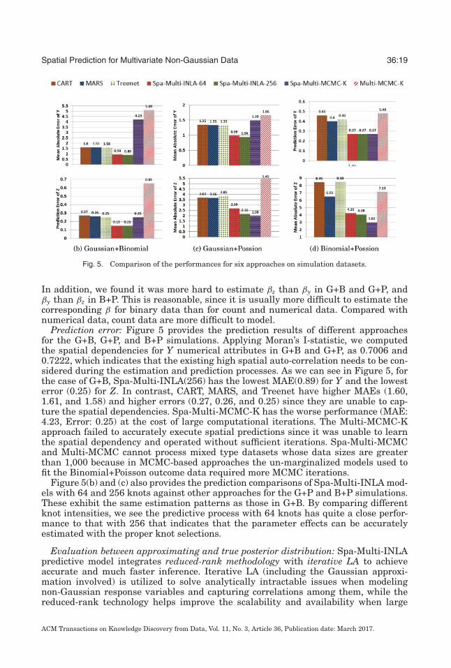
Fig. 5. Comparison of the performances for six approaches on simulation datasets.

In addition, we found it was more hard to estimate βz than βy in G+B and G+P, andβy than βz in B+P. This is reasonable, since it is usually more difficult to estimate thecorresponding β for binary data than for count and numerical data. Compared withnumerical data, count data are more difficult to model.

Prediction error: Figure 5 provides the prediction results of different approachesfor the G+B, G+P, and B+P simulations. Applying Moran’s I-statistic, we computedthe spatial dependencies for Y numerical attributes in G+B and G+P, as 0.7006 and0.7222, which indicates that the existing high spatial auto-correlation needs to be con-sidered during the estimation and prediction processes. As we can see in Figure 5, forthe case of G+B, Spa-Multi-INLA(256) has the lowest MAE(0.89) for Y and the lowesterror (0.25) for Z. In contrast, CART, MARS, and Treenet have higher MAEs (1.60,1.61, and 1.58) and higher errors (0.27, 0.26, and 0.25) since they are unable to cap-ture the spatial dependencies. Spa-Multi-MCMC-K has the worse performance (MAE:4.23, Error: 0.25) at the cost of large computational iterations. The Multi-MCMC-Kapproach failed to accurately execute spatial predictions since it was unable to learnthe spatial dependency and operated without sufficient iterations. Spa-Multi-MCMCand Multi-MCMC cannot process mixed type datasets whose data sizes are greaterthan 1,000 because in MCMC-based approaches the un-marginalized models used tofit the Binomial+Poisson outcome data required more MCMC iterations.

Figure 5(b) and (c) also provides the prediction comparisons of Spa-Multi-INLA mod-els with 64 and 256 knots against other approaches for the G+P and B+P simulations.These exhibit the same estimation patterns as those in G+B. By comparing differentknot intensities, we see the predictive process with 64 knots has quite a close perfor-mance to that with 256 that indicates that the parameter effects can be accuratelyestimated with the proper knot selections.

Evaluation between approximating and true posterior distribution: Spa-Multi-INLApredictive model integrates reduced-rank methodology with iterative LA to achieveaccurate and much faster inference. Iterative LA (including the Gaussian approxi-mation involved) is utilized to solve analytically intractable issues when modelingnon-Gaussian response variables and capturing correlations among them, while thereduced-rank technology helps improve the scalability and availability when large


36:20 X. Liu et al.

Table VI. Comparisons of Approximated and True Posterior Distribution in G+B��Approach

Paraβy βz φ σ 2

y σ 2z σ 2

yz τ 2 Time(s) MAEy Accz

True values

[0.600.60

] [0.150.15

]25 5.76 3.24 3.02 1.00 – – –

Spa-Multi-INLA(64)

[0.40(0.06)0.50(0.06)

] [−0.49(0.07)−0.07(0.01)

]8.38

(2.42)7.65

(3.87)2.60

(0.79)1.56

(1.10)1.49

(0.06)38.62 1.2495 0.7525

Spa-Multi-INLA-Full

[−2.13(0.15)−0.70(0.14)

] [−1.41(0.14)−4.38(0.13)

]19.59(4.20)

6.17(1.65)

4.81(1.67)

1.91(0.55)

0.99(0.07)

7082.41 1.1765 0.77

Spa-Multi-MCMC-Knots

[0.04(6.98)

−0.08(7.02)

] [−0.44(0.13)−0.19(0.13)

]18.73(3.04)

9.71(4.69)

0.01(0.29)

0.90(0.12)

0.11(0.14)

321.39 1.584 0.6375

amounts of data are being collected. Table VI evaluates the performances for param-eter estimation and prediction error of the Spa-Multi-INLA-Full (LA-based spatialmultivariate predictive model with full dataset), Spa-Multi-INLA(64) (LA-basedspatial multivariate predictive model with 64 knots) and Spa-Mulit-MCMC-Knots(MCMC-based spatial multivariate predictive model with 64 knots) models for oneGaussion+Binary simulation.

The best prediction results were generated by Spa-Multi-INLA-Full, which achievedperformances around 5% and 25% better than those of Spa-Multi-INLA(64) and Spa-Multi-MCMC-Knots(64), respectively. When estimating parameters, Spa-Multi-INLA-Full was able to capture spatial random effects across different locations more ac-curately. This can be verified by comparing the estimated values of σy, σz, and σyz,which exhibited improvements of 25% and more better than the knot-based approaches.Meanwhile, the Spa-Multi-INLA(64) was better modeling relationships between depen-dent and explanatory variables; its estimated values of βy and βz were around 20%–50%better than those generated by Spa-Multi-INLA-Full and Spa-Multi-MCMC-Knots.Theoretically, Spa-Multi-INLA-Full should have the best performance for spatial pre-dictive inference, because it models the predictive process with a far larger trainingdataset (1,000), while the knot-based approaches (Spa-Multi-INLA(64) and Spa-Multi-MCMC-knots) use only a relatively small number of points (64 of 1,000). However, inpractice this is not always the case. Since Spa-Multi-INLA is a complex model wheremany parameters are involved, the existence of outliers or noises requires the inferenceprocess to incorporate these into the model, which on occasion can mean that the spa-tial statistical model describes the random error as an underlying relationship. Thisoverfitting issue can adversely affect the estimation accuracy of several parameters.

Spa-Multi-INLA(64) has a similar parameter estimation and predictive capability tothat of the full predictive process. But there was a clear reduction in the computationcost when using the reduced-rank technique with the time required for the predictionprocess dropping from 7082.41 s (full process) to 38.62 s (knot-based process). Ifthere is an appropriate selection of knots that covers most of the domain knowledge,Gaussian and LA techniques can clearly provide accurate parameter estimation muchfaster. This approach has the added advantage of avoiding mistaking random errorsas underlying relationships, the well-known overfitting issue described above. Asshown in Table VI, when estimating βy and βz, Spa-Multi-INLA(64) better capturesthe relationship between the observed responses (Y and Z) and spatially referencedpredictors (X).

In order to measure the closeness of the approximated posterior distribution achievedby the new approach proposed here to the true posterior distribution, we calculatedthe root mean squared error (RMSE) values between the MAP estimation of model



Table VII. Comparison of RMSE on Estimated Parameters of Spa-Multi-INLA Among Different Data Sizes in G+B��Size

Para.βy βz φ σ 2

y σ 2z σ 2

yz τ2 Avg

200[0.27; 0.25

] [0.54; 0.57

]17.6 11.82 1.57 1.31 0.26 3.8

400[0.21; 0.18

] [0.35; 0.35

]17.66 9.73 1.29 1.25 0.36 3.48

600[0.14; 0.14

] [0.29; 0.3

]16.98 6.24 1.25 1.43 0.39 3.02

800[0.12; 0.12

] [0.22; 0.23

]16.83 4.4 1.27 1.54 0.41 2.79

1,000[0.11; 0.1

] [0.22; 0.2

]15.55 4.47 1.26 1.59 0.43 2.66

Table VIII. Settings in the Four Real Datasets

Dataset Size Ntr Nte Y Z Spatial dependence on YBEF spBayes[2012]

437 337 100 BE basal area EH basal area 0.1672

Lake Varinet al. [2005]

371 271 100 Troutabundance

Lake acidity 0.0072

MLST Dubin[1992]

211 150 61 House price If located in county 0.1753

House Pace andBarry [1997]

20,6402,0005,000

200500

House price House age 0.2529

parameters based on our approximated posterior and the true posterior. Because thetrue posterior is analytically intractable and it is difficult to evaluate the closenessto our approximated posterior at different sample sizes, we approximated the MAPestimation of the true posterior distribution by adjusting the parameters used to gen-erate the simulations. The comparison results shown in Table VII indicate that as thesample size increases, the MAP estimation of model parameters obtained using ournew approach becomes closer to the true model parameters.

Computational Cost: The last column in Tables III, IV, and V shows the comput-ing times required to deliver the estimation and prediction results for each of thesimulations. For the MCMC-based approaches, the main evaluation cost is the ma-trix inversion at O((2 ∗ 1000)3). For the Spa-Multi-INLA model, the main cost isO(2 ∗ n ∗ (2 ∗ m)2)(m = 64 or 256), which is the cost of building the required inverseand determinant of the size (2m+ 2p) × (2m+ 2p) matrix Q as shown in Equation (30),which assumes m � p. As shown in Tables III, IV and V, there is a clear reductionin the computational cost when using the Spa-Multi-INLA approach and the predic-tive process with 64 knots has a similar prediction capability but lower computationalburden compared to that 256 knots. Integrating the LA into the spatial multivariatepredictive model clearly helps achieve sufficiently five results in a moderate time.

6.2. Real-Life Datasets

We validated our approach using four real datasets, which are all G+B datasets.Table VIII summarizes the main information used in our experiment. The spatialdependencies were computed using Moran’s I-statistic function.

6.2.1. Experimental Results.Prediction error: Figure 6 summarizes the comparisons among Spa-Multi-INLA(64),

the four MCMC-based approaches, CART, MARS, and Treenet. The data name“Lake.271.100.1” indicates that it is the first realization generated from the original


36:22 X. Liu et al.

Fig. 6. Comparison of the performances for eight approaches on real-life datasets.

Lake data, with 271 training data and 100 test data points. By learning their spatialdependencies, we determined that most of the real datasets have lower spatial auto-correlations, which suggests that non-spatial attributes will contribute substantially tothe prediction of the outcome variables. For the predicted Y (numerical observations),the MAEs were computed to demonstrate the prediction performance. Neither Multi-MCMC nor Spa-Multi-MCMC could process the House data because of the large datasizes (2,000 and 5,000 points) involved. The MAE values from Spa-Multi-MCMC-K andMulti-MCMC-K were also much higher (around 10 times) than those (0.21–0.33) of theothers. When plotting the performance comparisons among Spa-Multi-INLA, CART,MARS, and Treenet, we did not include the MCMC-based plots for House as all theMCMC-based approaches generated poor results due to the large datasets involved(2,000 and 5,000), which incurred excessive computation times of around 2 days. In ourexperiments, the iteration values for all the datasets were set to 3,000, although thisstill cost around 1–3.5 hours with Multi-MCMC-K, and 2.5–4.5 hours with Spa-Multi-MCMC-K for the House datasets. As shown in Figure 6(a), Spa-Multi-INLA achieved anaverage 10% improvement over CART, MARA, and Treenet, 40–50% over Spa-Multi-MCMC-K and Spa-Multi-MCMC, and 60–70% over Multi-MCMC-K and Multi-MCMC.



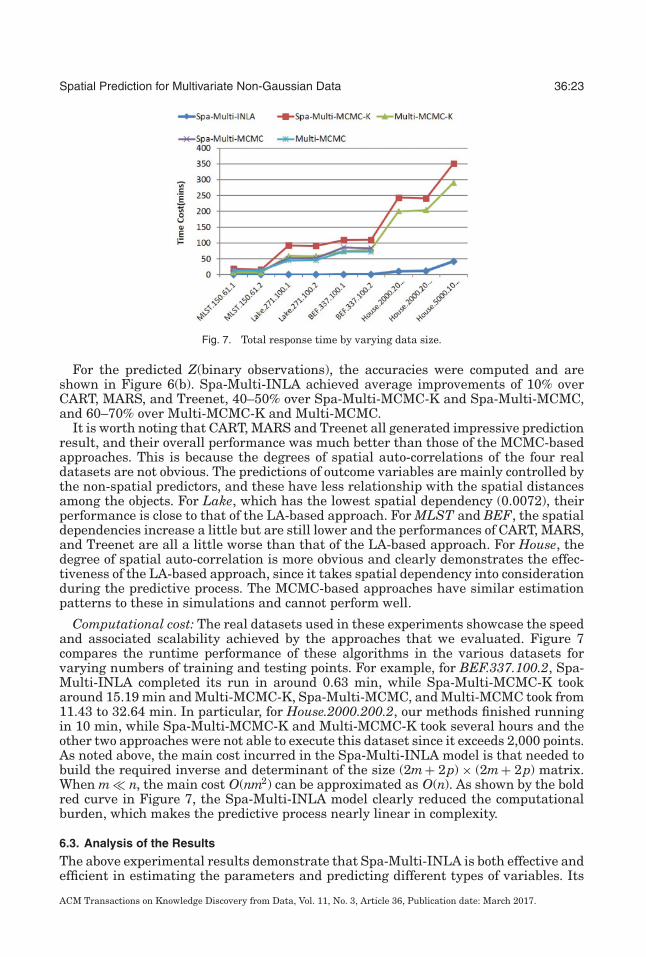
Fig. 7. Total response time by varying data size.

For the predicted Z(binary observations), the accuracies were computed and areshown in Figure 6(b). Spa-Multi-INLA achieved average improvements of 10% overCART, MARS, and Treenet, 40–50% over Spa-Multi-MCMC-K and Spa-Multi-MCMC,and 60–70% over Multi-MCMC-K and Multi-MCMC.

It is worth noting that CART, MARS and Treenet all generated impressive predictionresult, and their overall performance was much better than those of the MCMC-basedapproaches. This is because the degrees of spatial auto-correlations of the four realdatasets are not obvious. The predictions of outcome variables are mainly controlled bythe non-spatial predictors, and these have less relationship with the spatial distancesamong the objects. For Lake, which has the lowest spatial dependency (0.0072), theirperformance is close to that of the LA-based approach. For MLST and BEF, the spatialdependencies increase a little but are still lower and the performances of CART, MARS,and Treenet are all a little worse than that of the LA-based approach. For House, thedegree of spatial auto-correlation is more obvious and clearly demonstrates the effec-tiveness of the LA-based approach, since it takes spatial dependency into considerationduring the predictive process. The MCMC-based approaches have similar estimationpatterns to these in simulations and cannot perform well.

Computational cost: The real datasets used in these experiments showcase the speedand associated scalability achieved by the approaches that we evaluated. Figure 7compares the runtime performance of these algorithms in the various datasets forvarying numbers of training and testing points. For example, for BEF.337.100.2, Spa-Multi-INLA completed its run in around 0.63 min, while Spa-Multi-MCMC-K tookaround 15.19 min and Multi-MCMC-K, Spa-Multi-MCMC, and Multi-MCMC took from11.43 to 32.64 min. In particular, for House.2000.200.2, our methods finished runningin 10 min, while Spa-Multi-MCMC-K and Multi-MCMC-K took several hours and theother two approaches were not able to execute this dataset since it exceeds 2,000 points.As noted above, the main cost incurred in the Spa-Multi-INLA model is that needed tobuild the required inverse and determinant of the size (2m+ 2p) × (2m+ 2p) matrix.When m � n, the main cost O(nm2) can be approximated as O(n). As shown by the boldred curve in Figure 7, the Spa-Multi-INLA model clearly reduced the computationalburden, which makes the predictive process nearly linear in complexity.

6.3. Analysis of the Results

The above experimental results demonstrate that Spa-Multi-INLA is both effective andefficient in estimating the parameters and predicting different types of variables. Its


36:24 X. Liu et al.

Fig. 8. Prediction Performance of Spa-Multi-MCMC-K by varying iterations.

identification quality is clearly superior to that of existing techniques, achieving around10–30% improvement over CART, MARs, and Treetnet, and 40–50% over MCMC-basedapproaches. The experimental results verified three observations. (1) Appropriate KnotSelection. If there is an appropriate selection of knots that covers most of the domain ofinterest, the cost of the predictive process will be significantly reduced to a linear order.For the Spa-Multi-INLA model, the main cost is to compute the mode and Hessian ma-trix of the posterior distribution of latent variables, which costs O(n∗m2). When m � n,the predictive process becomes linear in complexity. (2) Efficient Approximation Pro-cess. When combined with numerical routines, Gaussian and LA techniques can providemuch faster and more accurate parameter estimation than MCMC-based algorithmsfor spatial multivariate non-Gaussian prediction. (3) Effectiveness for Large SpatialData Analysis. When processing more complicated datasets, such as the simulationdata shown in Figure 4, MCMC-based approaches need a very high number of iter-ations to achieve acceptable results, thus incurring unacceptably high computationalcosts, and CART MARS and Treenet cannot handle data with high spatial dependen-cies, but the new approach proposed here can complete the prediction computation inmoderate times with no loss of accuracy.

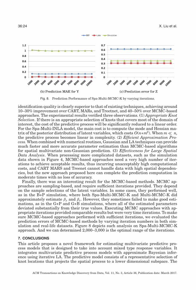
Finally, there was an interesting result for the MCMC-based methods. MCMC ap-proaches are sampling-based, and require sufficient iterations provided. They dependon the sample selections of the latent variables. In some cases, they performed well,as in the B+P simulation, where both Spa-Multi-MCMC-K and Multi-MCMC-K didapproximately estimate βy and βz. However, they sometimes failed to make good esti-mations, as in the G+P and G+B simulations, where all of the estimated parametersdeviated substantially from their true values. Executing MCMC approaches with ap-propriate iterations provided comparable results but were very time iterations. To makesure MCMC-based approaches performed with sufficient iterations, we evaluated theprediction errors of MCMC-based methods by varying iteration numbers in both sim-ulation and real-life datasets. Figure 8 depicts such analysis on Spa-Multi-MCMC-Kapproach. And we can determined 2,000–3,000 is the optimal range of the iterations.

7. CONCLUSIONS

This article proposes a novel framework for estimating multivariate predictive pro-cess models that is designed to take into account mixed type response variables. Itintegrates multivariate predictive process models with approximate Bayesian infer-ence using iterative LA. The predictive model consists of a representative selection ofknot locations that projects the spatial process to a lower dimensional subspace. The



approximation process provides more accurate and much faster inference for spatialmultivariate predictive models. Experimental results for synthetic and real datasetsconclusively demonstrated that our proposed non-Gaussian prediction model is capableof achieving a much higher processing capability in terms of prediction accuracy andcomputation time.

REFERENCES

T. C. Bailey and W. J. Krzanowski. 2000. Extensions to spatial factor methods with an illustration in geo-chemistry. Mathematical Geology 32, 6 (2000), 657–682. DOI:http://dx.doi.org/10.1023/A:1007589505425

S. Bandyopadhyay. 2005. Simulated annealing using a reversible jump Markov Chain Monte Carlo algorithmfor fuzzy clustering. IEEE Transactions on Knowledge and Data Engineering 17, 4 (2005), 479–490.

Sudipto Banerjee, Alan E. Gelfand, Andrew O. Finley, and Huiyan Sang. 2008. Gaussian predictive pro-cess models for large spatial data sets. Journal of the Royal Statistical Society: Series B (StatisticalMethodology) 70, 4 (2008), 825–848. DOI:http://dx.doi.org/10.1111/j.1467-9868.2008.00663.x

Mario Boley and Henrik Grosskreutz. 2008. A randomized approach for approximating the number of fre-quent sets. In Proceedings of the 2008 8th IEEE International Conference on Data Mining. 43–52.DOI:http://dx.doi.org/10.1109/ICDM.2008.85

Edwin V. Bonilla, Kian M. Chai, and Christopher Williams. 2008. Multi-task Gaussian process prediction.Advances in Neural Information Processing Systems, J. C. Platt, D. Koller, Y. Singer, and S. T. Roweis(Eds.). Vol. 20. Curran Associates, Inc., 153–160. http://papers.nips.cc/paper/3189-multi-task-gaussian-process-prediction.pdf.

Stephen Boyd and Lieven Vandenberghe. 2004. Convex Optimization. Cambridge University Press, NewYork, NY.

Leo Breiman, J. H. Friedman, R. A. Olshen, and C. J. Stone. 1984. Classification and Regression Trees.Wadsworth.

Catherine A. Calder. 2007. Dynamic factor process convolution models for multivariate space time data withapplication to air quality assessment. Environmental and Ecological Statistics 14, 3 (2007), 229–247.

Pierrette Chagneau, Frederic Mortier, Nicolas Picard, and Jean-NoAnl Bacro. 2010. HierarchicalBayesian model for Gaussian, Poisson and ordinal random fields. In Quantitative Geology and Geo-statistics, P. M. Atkinson and C. D. Lloyd (Eds.), Vol. 16. Springer, The Netherlands, 333–344.DOI:http://dx.doi.org/10.1007/978-90-481-2322-3_29

Pierrette Chagneau, Fradaric Mortier, Nicolas Picard, and Jean-Nol Bacro. 2011. A hierarchical Bayesianmodel for spatial prediction of multivariate non-Gaussian random fields. Biometrics 67, 1 (2011), 97–105.http://dx.doi.org/10.1111/j.1541-0420.2010.01415.x

Jorge Chica-Olmo. 2007. Prediction of housing location price by a multivariate spatial method: Cokriging.Journal of Real Estate Research 29, 1 (2007), 95–114.

Jungsoon Choi, Brian J. Reich, Montserrat Fuentes, and Jerry M. Davis. 2009. Multivariate spatial-temporal modeling and prediction of speciated fine particles 3, 2 (2009), 407–418. DOI:http://dx.doi.org/10.1080/15598608.2009.10411933

William F. Christensen and Yasuo Amemiya. 2001. Generalized shifted-factor analysis method for mul-tivariate geo-referenced data. Mathematical Geology 33, 7 (2001), 801–824. DOI:http://dx.doi.org/10.1023/A:1010998730645

William F. Christensen and Yasuo Amemiya. 2002. Latent variable analysis of multivariate spatial data.Journal of the American Statistical Association 97 (2002), 302–317.

Noel Cressie. 1991. Statistics for Spatial Data. Wiley-Interscience.N. Cressie and G. Johannesson. 2008. Fixed rank kriging for very large spatial data sets. Journal of the

Royal Statistical Society: Series B (Statistical Methodology) 70, 1 (2008), 209–226.Robin A. Dubin. 1992. Spatial autocorrelation and neighborhood quality. Regional Science and Urban Eco-

nomics 22, 3 (September 1992), 433–452.Andrew O. Finley, Huiyan Sang, Sudipto Banerjee, and Alan E. Gelfand. 2009. Improving the performance

of predictive process modeling for large datasets. Computational Statistics & Data Analysis 53, 8 (2009),2873–2884.

Jerome H. Friedman. 1991. Rejoinder: Multivariate adaptive regression splines. The Annals of Statistics 19,1 (1991), 123–141.

Jerome H. Friedman. 2000. Greedy function approximation: A gradient boosting machine. Annals of Statistics29 (2000), 1189–1232.


http://dx.doi.org/10.1023/A:1007589505425

http://dx.doi.org/10.1111/j.1467-9868.2008.00663.x

http://dx.doi.org/10.1109/ICDM.2008.85

http://dx.doi.org/10.1007/978-90-481-2322-3_29

http://dx.doi.org/10.1111/j.1541-0420.2010.01415.x

http://dx.doi.org/10.1080/15598608.2009.10411933

http://dx.doi.org/10.1080/15598608.2009.10411933

http://dx.doi.org/10.1023/A:1010998730645

http://dx.doi.org/10.1023/A:1010998730645

36:26 X. Liu et al.

A. E. Gelfand and S Banerjee. 2010. Multivariate spatial process models. In Handbook of Spatial Statistics.Chapman & Hall/CRC Press, 495–515.

A. E. Gelfand, A. M. Schmidt, S. Banerjee, and C. F. Sirmans. 2004. Nonstationary multivariate processmodeling through spatially varying coregionalization (with discussion). Test 13, 2 (2004), 1–50.

P. Goovaerts. 1997. Geostatistics for Natural Resources Evaluation. Oxford University Press, USA.Michel Grzebyk and Hans Wackernagel. 1994. Multivariateanalysis and spatial/temporal scales: Real and

complex models. Retrieved from http://citeseerx.ist.psu.edu/viewdoc/summary?doi=10.1.1.50.3893.Mikhail Kanevski. 2012. Multitask learning of environmental spatial data. In 6th International Congress on

Environmental Modelling and Software Society (iEMSs). Leipzig, Germany.B. M. Golam Kibria, Li Sun, James V. Zidek, and Nhu D. Le. 2002. Bayesian spatial prediction of random

space-time fields with application to mapping PM2.5 exposure. Journal of the American StatisticalAssociation 97 (2002), 112–124.

Guichong Li, Nathalie Japkowicz, Trevor J. Stocki, and R. Kurt Ungar. 2008. Border sampling throughcoupling Markov Chain Monte Carlo. (2008), 393–402. DOI:http://dx.doi.org/10.1109/ICDM.2008.52

Wei Liu, Yu Zheng, Sanjay Chawla, Jing Yuan, and Xie Xing. 2011. Discovering spatio-temporal causalinteractions in traffic data streams. In Proceedings of the 17th ACM SIGKDD International Con-ference on Knowledge Discovery and Data Mining (KDD’11). ACM, New York, NY, 1010–1018.DOI:http://dx.doi.org/10.1145/2020408.2020571

A. B. McBratney, I. O. A. Odeh, T. F. A. Bishop, M. S. Dunbar, and T. M. Shatar. 2005. An overview ofpedometric techniques for use in soil survey. Geoderma 97, 3–4 (2005), 293–327.

Marco Minozzo and Clarissa Ferrari. 2013. Multivariate geostatistical mapping of radioactive contaminationin the maddalena archipelago (Sardinia, italy): Spatial special issue. AStA Advances in StatisticalAnalysis 97, 2 (2013), 195–213. DOI:http://dx.doi.org/10.1007/s10182-012-0201-x

Marco Minozzo and Daniela Fruttini. 2004. Loglinear spatial factor analysis: An application to diabetesmellitus complications. Environmetrics 15, 5 (2004), 423–434. DOI:http://dx.doi.org/10.1002/env.675

Marco Minozzo and Laura Ferracuti. 2012. On the existence of some skew-normal stationary processes.Chilean Journal of Statistics 3 (2012), 157–170.

Seyed H. Mohammadi, Vandana Pursnani Janeja, and Aryya Gangopadhyay. 2009. Discretized spatio-temporal scan window. In Proceedings of the SIAM International Conference on Data Mining, SDM2009. 1195–1206. DOI:http://dx.doi.org/proceedings/datamining/2009/dm09_109_mohammadis.pdf

Daniel B. Neill and Andrew W. Moore. 2004. Rapid detection of significant spatial clusters. In Proceedings ofthe 10th ACM SIGKDD International Conference on Knowledge Discovery and Data Mining. 256–265.DOI:http://dx.doi.org/10.1145/1014052.1014082

Orlando Ohashi and Luıs Torgo. 2012. Spatial interpolation using multiple regression. In Proceedings ofICDM. 1044–1049.

Victor De Oliveira. 2000. Bayesian prediction of clipped Gaussian random fields. Computational Statisticsand Data Analysis 34, 3 (2000), 299–314.

Kelley Pace and Ronald Barry. 1997. Sparse spatial autoregressions. Statistics & Probability Letters 33, 3(1997), 291–297.

Gregory Piatetsky-Shapiro, Chabane Djeraba, Lise Getoor, Robert Grossman, Ronen Feldman, andMohammed Zaki. 2006. What are the grand challenges for data mining? KDD-2006 panel report.SIGKDD Explorations Newsletter 8, 2 (December 2006), 70–77. DOI:http://dx.doi.org/10.1145/1233321.1233330

Brian J. Reich and Montserrat Fuentes. 2007. A multivariate semiparametric Bayesian spatial modelingframework for hurricane surface wind fields. The Annals of Applied Statistics 1, 1 (2007), 249–264.

Qian Ren and Sudipto Banerjee. 2013. Hierarchical factor models for large spatially misaligned data: Alow-rank predictive process approach. Biometrics 69, 1 (2013), 19–30.

Greg Ridgeway and David Madigan. 2002. Bayesian analysis of massive datasets via particle filters. InProceedings of the 8th ACM SIGKDD International Conference on Knowledge Discovery and Data Mining(KDD’02). ACM, New York, NY, USA, 5–13.

Havard Rue and Leonhard Held. 2005. Gaussian Markov Random Fields: Theory and Applications, Mono-graphs on Statistics and Applied Probability, Vol. 104. Chapman & Hall, London.

Havard Rue, Sara Martino, and Nicolas Chopin. 2009. Approximate Bayesian inference for latentGaussian models by using integrated nested laplace approximations. Journal of the Royal Statis-tical Society: Series B (Statistical Methodology) 71, 2 (2009), 319–392. DOI:http://dx.doi.org/10.1111/j.1467-9868.2008.00700.x

A. Schmidt and M. Rodriguez. 2011. Modelling multivariate counts varying continuously in space. BayesianStatistic (2011).


http://citeseerx.ist.psu.edu/viewdoc/summary?doi$=$10.1.1.50.3893

http://dx.doi.org/10.1109/ICDM.2008.52

http://dx.doi.org/10.1145/2020408.2020571

http://dx.doi.org/10.1007/s10182-012-0201-x

http://dx.doi.org/10.1002/env.675

http://dx.doi.org/proceedings/datamining/2009/dm09_109_mohammadis.pdf

http://dx.doi.org/10.1145/1014052.1014082

http://dx.doi.org/10.1145/1233321.1233330

http://dx.doi.org/10.1145/1233321.1233330

http://dx.doi.org/10.1111/j.1467-9868.2008.00700.x

http://dx.doi.org/10.1111/j.1467-9868.2008.00700.x


Salford Systems. 2017. Homepage. Retrieved from http://www.salford-systems.com/.spBayes. 2012. spBayes: Univariate and multivariate spatial modeling. Retrieved from http://cran.r-project.

org/web/packages/spBayes/.Luis Torgo and Orlando Ohashi. 2011. 2D-interval predictions for time series. In Proceedings of the 17th

ACM SIGKDD International Conference on Knowledge Discovery and Data Mining (KDD’11). ACM, NewYork, NY, 787–794. DOI:http://dx.doi.org/10.1145/2020408.2020546

Cristiano Varin, Gudmund Host, and Oivind Skare. 2005. Pairwise likelihood inference in spatial generalizedlinear mixed models. Computational Statistics & Data Analysis 49, 4 (June 2005), 1173–1191.

H. Wackernagel. 2003. Multivariate Geostatistics: An Introduction with Applications (2nd ed.). Springer-Verlag. 381.

F. Wang and M. M. Wall. 2003. Generalized common spatial factor model. Biostatistics (Oxford, England) 4,4 (October 2003), 569–582.

R. Webster and M. A. Oliver. 1990. Statistical Methods in Soil and Land Resource Survey. Oxford UniversityPress, 316.

M. A. Wibrin, P. Bogaert, and D. Fasbender. 2006. Combining categorical and continuous spatial informa-tion within the Bayesian Maximum Entropy paradigm. Stochastic Environmental Research and RiskAssessment 20, 6 (2006), 423–433.

Robert L. Wolpert and Katja Ickstadt. 1997. Poisson/gamma random field models for spatial statistics.Biometrika 85, 2 (1997), 251–267.

Elizabeth Wu, Wei Liu, and Sanjay Chawla. 2008. Spatio-temporal outlier detection in precipitation data.In Proceedings of the KDD Workshop on Knowledge Discovery from Sensor Data. 115–133.

Mingxi Wu, Chris Jermaine, Sanjay Ranka, Xiuyao Song, and John Gums. 2010. A model-agnostic frameworkfor fast spatial anomaly detection. TKDD 4, 4 (2010), 20.

Mingxi Wu, Xiuyao Song, Chris Jermaine, Sanjay Ranka, and John Gums. 2009. A LRT framework forfast spatial anomaly detection. In Proceedings of the 15th ACM SIGKDD International Conferenceon Knowledge Discovery and Data Mining. Paris, France, 887–896. DOI:http://doi.acm.org/10.1145/1557019.1557116

Harry Zhang and Shengli Sheng. 2004. Learning weighted naive Bayes with accurate ranking. In Proceedingsof the Fourth IEEE International Conference on Data Mining. 567–570.

J. Zhu, J. C. Eickhoff, and P. Yan. 2005. Generalized linear latent variable models for repeated mea-sures of spatially correlated multivariate data. Biometrics 61, 3 (2005), 674–683. DOI:http://dx.doi.org/10.1111/j.1541-0420.2005.00343.x

Wei Zhuo, Prabhat, Chris Paciorek, Cari Kaufman, and Wes Bethel. 2011. Parallel kriging analysis for largespatial datasets. In Proceedings of ICDM Workshops’11. 38–44.

Received November 2014; revised May 2015; accepted November 2016


http://www.salford-systems.com/

http://cran.r-project.org/web/packages/spBayes/

http://cran.r-project.org/web/packages/spBayes/

http://dx.doi.org/10.1145/2020408.2020546

http://doi.acm.org/10.1145/1557019.1557116

http://doi.acm.org/10.1145/1557019.1557116

http://dx.doi.org/10.1111/j.1541-0420.2005.00343.x

http://dx.doi.org/10.1111/j.1541-0420.2005.00343.x

Date post:	23-Mar-2022
Category:	Documents
Upload:	others
View:	8 times
Download:	0 times

36 Spatial Prediction for Multivariate Non-Gaussian Data

Documents