3D Face Mask Presentation Attack Detection Based on ... · 3D Face Mask Presentation Attack...

3D Face Mask Presentation Attack Detection Based onIntrinsic Image Analysis

Lei Lia, Zhaoqiang Xiaa, Xiaoyue Jianga, Yupeng Maa, Fabio Rolib,a, Xiaoyi Fenga

aSchool of Electronics and Information, Northwestern Polytechnical University, Xi’an, Shaanxi, ChinabDepartment of Electrical and Electronic Engineering, University of Cagliari, Cagliari, Sardinia, Italy

Abstract

Face presentation attacks have become a major threat to face recognition systems and

many countermeasures have been proposed in the past decade. However, most of them

are devoted to 2D face presentation attacks, rather than 3D face masks. Unlike the real

face, the 3D face mask is usually made of resin materials and has a smooth surface,

resulting in reflectance differences. So, we propose a novel detection method for 3D

face mask presentation attack by modeling reflectance differences based on intrinsic

image analysis. In the proposed method, the face image is first processed with intrinsic

image decomposition to compute its reflectance image. Then, the intensity distribu-

tion histograms are extracted from three orthogonal planes to represent the intensity

differences of reflectance images between the real face and 3D face mask. After that,

the 1D convolutional network is further used to capture the information for describing

different materials or surfaces react differently to changes in illumination. Extensive

experiments on the 3DMAD database demonstrate the effectiveness of our proposed

method in distinguishing a face mask from the real one and show that the detection

performance outperforms other state-of-the-art methods.

Keywords: 3D face PAD, Intrinsic Image Analysis, Deep Learning

1. Introduction

Face presentation attack detection (PAD) has become an important issue in face

recognition, since the biometric technologies have been applied in various verification

systems and mobile devices. For instance, Apple’s face ID for iPhone X has been

Preprint submitted to Elsevier March 28, 2019

arX

iv:1

903.

1130

3v1

[cs

.CV

] 2

7 M

ar 2

019

used to unlock cell phones and complete mobile payments. However, D. Oberhaus [1]

reported that some researchers at the Vietnamese cybersecurity firm Bkav had made a

mask that could fool the Face ID system. Considering such urgent security situation,

an effective and reliable 3D face mask PAD method must be developed.

Based on different presented fake faces, four kinds of presentation attacks can be

considered: printed photo, displayed image, replayed video and 3D mask. The printed

photo, displayed image and replayed video attacks usually print or display a face im-

age in 2D medium (e.g., paper and LCD screen). But for 3D face mask scenario, the

attacker wears a 3D mask to deceive face recognition system. Compared to 2D face

presentation attacks, 3D face masks contain the structural and depth information simi-

lar to real faces. Fig. 1 shows an example of different face presentation attacks.

In the last decade, many face PAD approaches have been proposed [2, 3, 4, 5, 6,

7, 8, 9, 10, 11, 12, 13]. However, the main focus of them has been on tackling the

problem of 2D face presentation attacks, while 3D attacks have received much less

attention. It is because detecting 3D face masks and distinguish them from real faces

more challenging for common cameras. For instance, Liu et al. [14] estimated face

depth by a CNN-RNN model and used the depth information to detect presented fake

faces. This method can solve the 2D face PAD successfully. Whereas, this detection

method cannot work well in a 3D mask attack as the mask also has depth information.

In another work, Li et al. [15] tackled the 3D mask attacks by detecting the pulse from

videos, which may be sensitive to camera settings and light conditions. Besides, it

becomes easier to obtain 3D masks by attackers with the development of 3D printing.

Thus, it is necessary to develop new methods for detecting 3D face mask.

In this work, we propose to analyze the intrinsic image for 3D face mask PAD.

Intrinsic image decomposition can divide a single image into a reflectance image and a

shading image [16]. For the reflectance image, it gives the albedo at each point, which

describes the reflectance characteristics and is only decided by the material itself. In

contrast, the shading image gives the total light flux incident at each point. Comparing

the real face with face mask, we can find that their constituted materials are fairly

different. Furthermore, due to the influence of hair follicles, the surface of 3D face

mask is smoother than the surface of real face. More specifically, the face skin consists

2

Figure 1: Samples of face presentation attacks. From left to right: printed face photos, displayed face images

or replayed videos, and 3D masks.

describes the reflectance characteristics and is only decided by the material itself. In

contrast, the shading image gives the total light flux incident at each point. Comparing

the real face with face mask, we can find that their constituted materials are fairly

different. Furthermore, due to the influence of hair follicles, the surface of 3D face

mask is smoother than the surface of real face. More specifically, the face skin consists35

of three layers: epidermis, dermis and subcutaneous fat 1 as illustrated in Fig. 2 (left).

But for the 3D face mask, it is often made of resin materials as shown in Fig. 2 (right).

These material or surface differences can be revealed in reflectance images and further

used for analyzing visual difference.

Our proposed method can be divided into three procedures: (i) the captured face40

image is first decomposed into a reflectance image and a shading image based on

correlation-based intrinsic image extraction (CIIE) [17]; (ii) the intensity distribution

histograms of reflectance images are calculated from three orthogonal planes and the

1D convolutional neural network (CNN) is introduced to extract the differences in re-

flectance images; (iii) the extracted features are fed into a Support Vector Machine45

(SVM) classifier to detect 3D face mask attack. The main contributions of this work

1https://www.webmd.com/skin-problems-and-treatments/ss/slideshow-skin-infections

3

Figure 1: Samples of face presentation attacks. From left to right: printed face photos, displayed face images

or replayed videos, and 3D masks.

of three layers: epidermis, dermis and subcutaneous fat 1 as illustrated in Fig. 2 (left).

But for the 3D face mask, it is often made of resin materials as shown in Fig. 2 (right).

These material or surface differences can be revealed in reflectance images and further

used for analyzing visual difference.

Our proposed method can be divided into three procedures: (i) the captured face

image is first decomposed into a reflectance image and a shading image based on

correlation-based intrinsic image extraction (CIIE) [17]; (ii) the intensity distribution

histograms of reflectance images are calculated from three orthogonal planes and the

1D convolutional neural network (CNN) is introduced to extract the differences in re-

flectance images; (iii) the extracted features are fed into a Support Vector Machine

(SVM) classifier to detect 3D face mask attack. The main contributions of this work

are summarized:

� Unlike most previous works on 3D face mask PAD are based on analyzing visible

cues (e.g. texture) directly, we propose a novel and appealing countermeasure from the

view of intrinsic image decomposition.

� We design an intensity distribution feature for describing the difference of re-

1https://www.webmd.com/skin-problems-and-treatments/ss/slideshow-skin-infections

3

Face skin Resin

Face MaskReal Face

Figure 2: The difference between real face (left) and face mask (right) in skin material. For the real face

skin, it consists of three layers: epidermis, dermis and subcutaneous fat. But for the face mask, it is often

made of resin materials.

are summarized:

⋄ Unlike most previous works on 3D face mask PAD are based on analyzing visible

cues (e.g. texture) directly, we propose a novel and appealing countermeasure from the

view of intrinsic image decomposition.50

⋄ We design an intensity distribution feature for describing the difference of re-

flectance images between the real face and 3D face mask and introduce 1D CNN to

represent different materials or surfaces react differently to the changes in variational

illumination.

⋄ We evaluate the proposed method on 3DMAD dataset and achieve the state-of-55

the-art performance.

2. Related Work

2.1. Methods for 2D Face PAD

Texture-analysis based methods. Due to the limitations of printers and display de-

vices, the printed or replayed fake faces generally present blurred textures compared to60

4

Figure 2: The difference between real face (left) and face mask (right) in skin material. For the real face

skin, it consists of three layers: epidermis, dermis and subcutaneous fat. But for the face mask, it is often

made of resin materials.

flectance images between the real face and 3D face mask and introduce 1D CNN to

represent different materials or surfaces react differently to the changes in variational

illumination.

� We evaluate the proposed method on 3DMAD dataset and achieve the state-of-

the-art performance.

2. Related Work

2.1. Methods for 2D Face PAD

Texture-analysis based methods. Due to the limitations of printers and display de-

vices, the printed or replayed fake faces generally present blurred textures compared to

the real ones. Thus, using texture information has been a natural approach to tackling

2D face presentation attack. For instance, many works employed hand-crafted features,

such as local binary pattern (LBP) [4], Haralick features [18] and scale-invariant feature

transform (SIFT) [19], and then used traditional classifiers, such as SVM and LDA. To

capture the color differences in chrominance, the texture features extracted from differ-

4

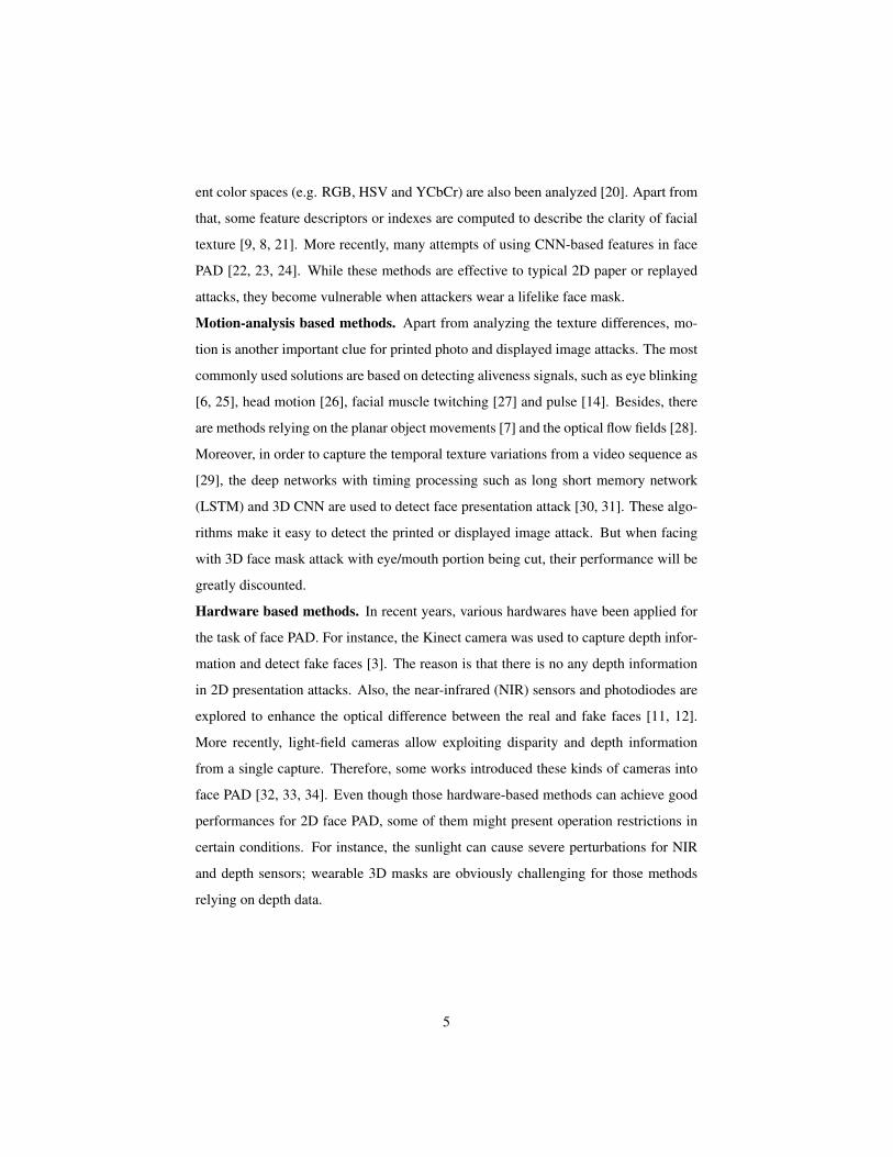
ent color spaces (e.g. RGB, HSV and YCbCr) are also been analyzed [20]. Apart from

that, some feature descriptors or indexes are computed to describe the clarity of facial

texture [9, 8, 21]. More recently, many attempts of using CNN-based features in face

PAD [22, 23, 24]. While these methods are effective to typical 2D paper or replayed

attacks, they become vulnerable when attackers wear a lifelike face mask.

Motion-analysis based methods. Apart from analyzing the texture differences, mo-

tion is another important clue for printed photo and displayed image attacks. The most

commonly used solutions are based on detecting aliveness signals, such as eye blinking

[6, 25], head motion [26], facial muscle twitching [27] and pulse [14]. Besides, there

are methods relying on the planar object movements [7] and the optical flow fields [28].

Moreover, in order to capture the temporal texture variations from a video sequence as

[29], the deep networks with timing processing such as long short memory network

(LSTM) and 3D CNN are used to detect face presentation attack [30, 31]. These algo-

rithms make it easy to detect the printed or displayed image attack. But when facing

with 3D face mask attack with eye/mouth portion being cut, their performance will be

greatly discounted.

Hardware based methods. In recent years, various hardwares have been applied for

the task of face PAD. For instance, the Kinect camera was used to capture depth infor-

mation and detect fake faces [3]. The reason is that there is no any depth information

in 2D presentation attacks. Also, the near-infrared (NIR) sensors and photodiodes are

explored to enhance the optical difference between the real and fake faces [11, 12].

More recently, light-field cameras allow exploiting disparity and depth information

from a single capture. Therefore, some works introduced these kinds of cameras into

face PAD [32, 33, 34]. Even though those hardware-based methods can achieve good

performances for 2D face PAD, some of them might present operation restrictions in

certain conditions. For instance, the sunlight can cause severe perturbations for NIR

and depth sensors; wearable 3D masks are obviously challenging for those methods

relying on depth data.

5

2.2. Methods for 3D Face Mask PAD

3D face mask presentation attack is a new threat to face biometric systems and few

countermeasures have been proposed compared to conventional 2D attacks. To address

this issue, Erdogmus et al. [35] released the first 3D mask attack dataset (3DMAD).

Different from printed or replayed fake faces, the attackers in 3DMAD wear 3D face

masks of targeted persons. Inspired by [4], Erdogmus et al. utilized multi-scale LBP

based texture representation for 3D face mask PAD. In addition, Liu et al. [36] pre-

sented an rPPG-based method to cope with 3D mask attacks. In another work, Li et al.

[15] tackled the 3D mask attacks based on pulse detection. These two methods mainly

analyze the different heartbeat signals between real faces and 3D masks. However,

they may be sensitive to camera settings and light conditions. More recently, Shao et

al. [37] extracted optical flow features from a pre-trained VGG-net [38] to estimate

subtle motion.

3. Proposed Method

3.1. Rationale and Motivations

As aforementioned, the constituted materials of real face and 3D face mask are

different and these differences can be revealed in reflectance images, which are shown

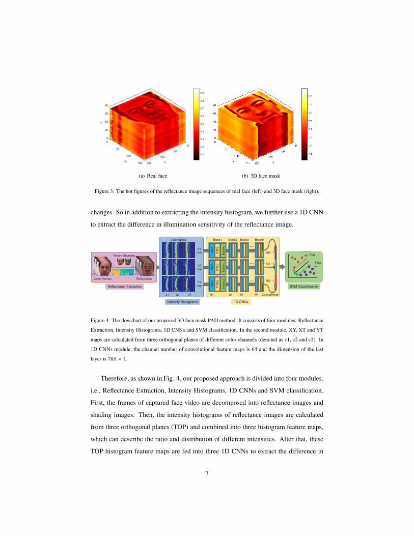
in Fig. 3(a) and 3(b). From the example, it can be found that the reflectance images of

real face have low intensity and uniform distribution while the reflectance images of 3D

face mask have high intensity and non-uniform distribution. Based on this observation,

we propose a new method to discriminate the reflectance difference of real faces and

3D face masks.

In reflectance images of real and spoofing faces, reflectance images often present

obvious intensity difference due to different materials and surface structures. To de-

scribe the intensity differences, we extract intensity histograms from the view of albedo

intensity. Furthermore, the skin surface of the real face is rougher than the 3D face

mask, which is caused by hair follicles, etc. When lighting changes or the face shake,

the reflectance images of real face and 3D face mask also show different responses.

For instance, the reflectance image of a smooth surface is more sensitive to lighting

6

(a) Real face (b) 3D face mask

Figure 3: The hot figures of the reflectance image sequences of real face (left) and 3D face mask (right).

mask, which is caused by hair follicles, etc. When lighting changes or the face shake,120



changes. So in addition to extracting the intensity histogram, we further use a 1D CNN

to extract the difference in illumination sensitivity of the reflectance image.

Reflectance Extraction

75 75

Video Frames Reflectance

Intensity Histograms

XY

map

XT

map

YT

map

Conv

ReLU

Poolin

g

Conv

ReLU

Poolin

g

Conv

ReLU

Poolin

g

1D CNNs

SVM Classification

Real

Fake

Texture Segment

c1 c2 c3 Concatenate64 6464 64

Color Space Block1 Block2 Block3 Block6

768 1

768 1

768 1

Figure 4: The flowchart of our proposed 3D face mask PAD method. It consists of four modules: Reflectance

Extraction, Intensity Histograms, 1D CNNs and SVM classification. In the second module, XY, XT and YT

maps are calculated from three orthogonal planes of different color channels (denoted as c1, c2 and c3). In

1D CNNs module, the channel number of convolutional feature maps is 64 and the dimension of the last

layer is 768 × 1.

Therefore, as shown in Fig. 4, our proposed approach is divided into four modules,125

i.e., Reflectance Extraction, Intensity Histograms, 1D CNNs and SVM classification.

First, the frames of captured face video are decomposed into reflectance images and

shading images. Then, the intensity histograms of reflectance images are calculated

7

(a) Real face(a) Real face (b) 3D face mask








75 75



XY

map

XT

map

YT

map

Conv

ReLU

Poolin

g

Conv

ReLU

Poolin

g

Conv

ReLU

Poolin

g

1D CNNs

SVM Classification

Real

Fake

Texture Segment



768 1

768 1

768 1





layer is 768 × 1.





7

(b) 3D face mask




(a) Real face (b) 3D face mask








75 75



XY

map

XT

map

YT

map

Conv

ReLU

Poolin

g

Conv

ReLU

Poolin

g

Conv

ReLU

Poolin

g

1D CNNs

SVM Classification

Real

Fake

Texture Segment



768 1

768 1

768 1





layer is 768 × 1.





7





layer is 768× 1.

Therefore, as shown in Fig. 4, our proposed approach is divided into four modules,




from three orthogonal planes (TOP) and combined into three histogram feature maps,

which can describe the ratio and distribution of different intensities. After that, these

TOP histogram feature maps are fed into three 1D CNNs to extract the difference in

7

illumination sensitivity, respectively. Finally, an SVM classifier is employed to distin-

guish whether the concatenated deep features are oriented from a valid access or a 3D

face mask.

3.2. Intrinsic Image Decomposition

Based on the Lambertian theory [16], the intensity value I(x, y) of every pixel in

an image is the product of the shading S(x, y) and the reflectanceR(x, y) at that point:

I(x, y) = S(x, y) × R(x, y). The shading S(x, y) represents illumination changes

and is decided by external light intensity. R(x, y) gives the albedo at each point. In

addition, albedo completely describes the reflectance characteristics for Lambertian

(perfectly diffusing) surfaces. Considering different materials of real face and 3D face

mask, we will analyze the reflectance images of them. In the context, we utilize the

CIIE algorithm [17] to decompose the original face image.

More specifically, the steerable filters are first used to decompose the face image

into its constituent orientation/frequency bands. Then, the filter bank is applied to es-

timate the luminance components (LMij) and the variations in local amplitude (AM ),

texture (TM ), and hue (HM ), respectively. Based on this assumption that luminance

variations are either due to reflectance or illumination but not both, the estimated shad-

ing and reflectance can be reconstructed as follows:

S = FS ⊗

Crec shdij × LMij ifCrec shd

ij > 0

0 ifCrec shdij ≤ 0

(1)

R = FS ⊗

Crec refij × LMij ifCrec ref

ij > 0

0 ifCrec refij ≤ 0

(2)

where ij is the index of LM and ⊗ is the reconstruction of steerable filters FS with

weighted LMij . Crec shdij and Crec ref

ij are correlation coefficients for reconstructed

shading and reflectance, respectively.

During image reconstruction, some LM components will be set to zero and re-

sulting images may lose their DC values. Meanwhile, some AM components will

represent small variations in reflectance not shading. Thus two cost functions are used

8

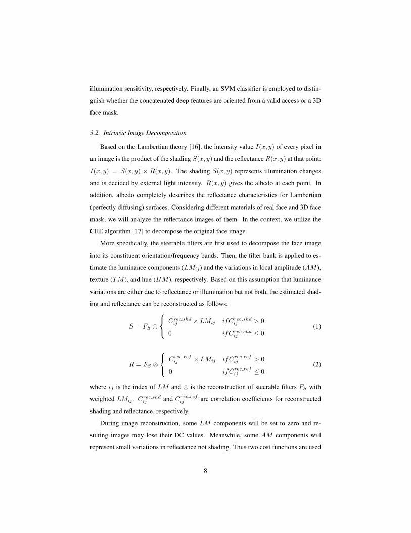
to optimize S and R, as illustrated in Eq. 3 and Eq. 4.

ES(VDC) = argminTi

∑

i

Ftxt(I

S + VDC, Ti) (3)

ER = argmink∑

i

Ftxt( ˆLM ij , Tk) + λEcst(Fadj) (4)

where VDC is the DC value to be optimized. The function Ftxt(I , Ti) represents texture

consistency evaluated for image I against the texture segmentation result. ˆLM ij is

modelled as a normal distribution and Ecst(Fadj) constrains the maximum rescaling

produced by the adjustment function. Fig. 3 shows the reflectance image sequences of

a real face and a 3D face mask.

Table 1: The configuration parameters in 1D CNN. aPool is the operation of average pooling and Trans is

the operation of matrix transpose.layer 1 2 3 4 5 6 7 8 9 10 11

type Conv ReLU aPool Conv ReLU aPool Conv ReLU aPool Conv ReLU

filt size [3, 1] − − [3, 1] − − [3, 1] − − [3, 1] −filt dim 1 − − 64 − − 64 − − 64 −

num filts 64 − − 64 − − 64 − − 64 −stride 1 1 [2, 1] 1 1 [2, 1] 1 1 [2, 1] 1 1

pad [1, 0] 0 0 [1, 0] 0 0 [1, 0] 0 0 [1, 0] 0

layer 12 13 14 15 16 17 18 19 20 21 22

type aPool Conv ReLU aPool Conv ReLU Conv Trans FC SoftMax −

filt size − [3, 1] − − [2, 1] − [1, 1] − [1, 1] − −filt dim − 64 − − 64 − 64 − 64 − −

num filts − 64 − − 64 − 64 − 2 − −stride [2, 1] 1 1 [2, 1] 1 1 1 1 1 1 −pad 0 [1, 0] 0 0 0 0 0 0 0 0 −

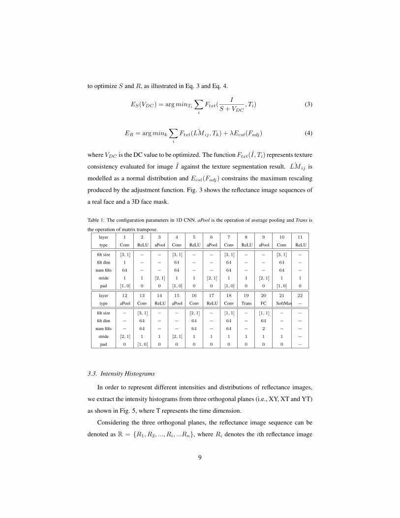
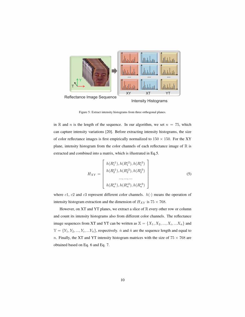
3.3. Intensity Histograms

In order to represent different intensities and distributions of reflectance images,

we extract the intensity histograms from three orthogonal planes (i.e., XY, XT and YT)

as shown in Fig. 5, where T represents the time dimension.

Considering the three orthogonal planes, the reflectance image sequence can be

denoted as R = {R1, R2, ..., Ri, ...Rn}, where Ri denotes the ith reflectance image

9

Y

T

XY XT YTReflectance Image Sequence


Figure 5: Extract intensity histograms from three orthogonal planes.

Considering the three orthogonal planes, the reflectance image sequence can be

denoted as R = {R1, R2, ..., Ri, ...Rn}, where Ri denotes the ith reflectance image

in R and n is the length of the sequence. In our algorithm, we set n = 75, which170

can capture intensity variations [20]. Before extracting intensity histograms, the size

of color reflectance images is first empirically normalized to 150 × 150. For the XY

plane, intensity histogram from the color channels of each reflectance image of R is

extracted and combined into a matrix, which is illustrated in Eq.5.

HXY =

h(Rc11 ), h(Rc2

1 ), h(Rc31 )

h(Rc12 ), h(Rc2

2 ), h(Rc32 )

..., ..., ...

h(Rc1n ), h(Rc2

n ), h(Rc3n )

(5)

where c1, c2 and c3 represent different color channels. h(·) means the operation of175

intensity histogram extraction and the dimension of HXY is 75 × 768.

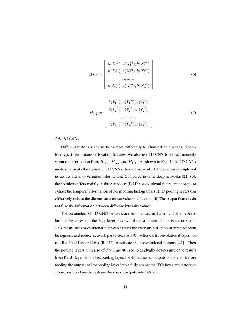
However, on XT and YT planes, we extract a slice of R every other row or column

and count its intensity histograms also from different color channels. The reflectance

image sequences from XT and YT can be written as X = {X1, X2, ..., Xi, ...Xn} and

Y = {Y1, Y2, ..., Yi, ...Yn}, respectively. n and n are the sequence length and equal to180

n. Finally, the XT and YT intensity histogram matrices with the size of 75 × 768 are

obtained based on Eq. 6 and Eq. 7.

10

Figure 5: Extract intensity histograms from three orthogonal planes.

in R and n is the length of the sequence. In our algorithm, we set n = 75, which

can capture intensity variations [20]. Before extracting intensity histograms, the size

of color reflectance images is first empirically normalized to 150 × 150. For the XY

plane, intensity histogram from the color channels of each reflectance image of R is

extracted and combined into a matrix, which is illustrated in Eq.5.

HXY =

h(Rc11 ), h(Rc2

1 ), h(Rc31 )

h(Rc12 ), h(Rc2

2 ), h(Rc32 )

..., ..., ...

h(Rc1n ), h(Rc2

n ), h(Rc3n )

(5)

where c1, c2 and c3 represent different color channels. h(·) means the operation of

intensity histogram extraction and the dimension of HXY is 75× 768.

However, on XT and YT planes, we extract a slice of R every other row or column

and count its intensity histograms also from different color channels. The reflectance

image sequences from XT and YT can be written as X = {X1, X2, ..., Xi, ...Xn} and

Y = {Y1, Y2, ..., Yi, ...Yn}, respectively. n and n are the sequence length and equal to

n. Finally, the XT and YT intensity histogram matrices with the size of 75 × 768 are

obtained based on Eq. 6 and Eq. 7.

10

HXT =

h(Xc11 ), h(Xc2

1 ), h(Xc31 )

h(Xc12 ), h(Xc2

2 ), h(Xc32 )

..., ..., ...

h(Xc1n ), h(Xc2

n ), h(Xc3n )

(6)

HY T =

h(Y c11 ), h(Y c2

1 ), h(Y c31 )

h(Y c12 ), h(Y c2

2 ), h(Y c32 )

..., ..., ...

h(Y c1n ), h(Y c2

n ), h(Y c3n )

(7)

3.4. 1D CNNs

Different materials and surfaces react differently to illumination changes. There-

fore, apart from intensity location features, we also use 1D CNN to extract intensity

variation information from HXY , HXT and HY T . As shown in Fig. 4, the 1D CNNs

module presents three parallel 1D CNNs. In each network, 1D operation is employed

to extract intensity variation information. Compared to other deep networks [22, 39],

the solution differs mainly in three aspects: (i) 1D convolutional filters are adopted to

extract the temporal information of neighboring histograms; (ii) 1D pooling layers can

effectively reduce the dimension after convolutional layers; (iii) The output features do

not fuse the information between different intensity values.

The parameters of 1D CNN network are summarized in Table 1. For all convo-

lutional layers except the 16th layer, the size of convolutional filters is set to 3 × 1.

This means the convolutional filter can extract the intensity variation in three adjacent

histograms and reduce network parameters as [40]. After each convolutional layer, we

use Rectified Linear Units (ReLU) to activate the convolutional outputs [41]. Then

the pooling layers with size of 2 × 1 are utilized to gradually down-sample the results

from ReLU layer. In the last pooling layer, the dimension of outputs is 1×768. Before

feeding the outputs of last pooling layer into a fully connected (FC) layer, we introduce

a transposition layer to reshape the size of outputs into 768× 1.

11

100 200 300 400 500 600 700

10

20

30

40

50

60

70

0

0.005

0.01

0.015

0.02

0.025

(a) Real face: XY histogram matrix

0 100 200 300 400 500 600 700 800-12

-10

-8

-6

-4

-2

0

2

(b) Real face: Output of 1D CNN

100 200 300 400 500 600 700

10

20

30

40

50

60

70

0

0.002

0.004

0.006

0.008

0.01

0.012

0.014

0.016

0.018

0.02

(c) 3D mask: XY histogram matrix

0 100 200 300 400 500 600 700 800-10

-8

-6

-4

-2

0

2

(d) 3D mask: Output of 1D CNN

Figure 6: The input and output of 1D CNN network. (a) and (b) are the results of a real face reflectance

image sequence, and (c) and (d) are the results of a 3D face mask reflectance image sequence. To make the

histogram matrix better visualized, we use jet colormap in (a) and (c). (b) and (d) plot the area of the output

of 1D CNNs.

For face PAD, its essence is to classify whether the input is a real face or a pre-

sented 3D face mask. Thus, after FC layer, the most commonly used SoftMax loss

function is employed to train the network parameters [42]. In testing stage, we extract

the outputs of the last Conv layer as the finally features of HXY , HXT and HY T de-205

noted as CXY , CXT and CY T . Fig. 6 shows the intensity histogram matrixes and the

learned intensity variation features of the reflectance image sequences of the real face

and the 3D face mask in XY plane of RGB color space. After feature extraction, we

concatenate CXY , CXT and CY T into a feature vector with stronger representation,

which are fed into an SVM classifier.210

In training stage, the stochastic gradient descent (SGD) algorithm [43] is used to

12


100 200 300 400 500 600 700

10

20

30

40

50

60

70

0

0.005

0.01

0.015

0.02

0.025


0 100 200 300 400 500 600 700 800-12

-10

-8

-6

-4

-2

0

2


100 200 300 400 500 600 700

10

20

30

40

50

60

70

0

0.002

0.004

0.006

0.008

0.01

0.012

0.014

0.016

0.018

0.02


0 100 200 300 400 500 600 700 800-10

-8

-6

-4

-2

0

2





of 1D CNNs.











12


100 200 300 400 500 600 700

10

20

30

40

50

60

70

0

0.005

0.01

0.015

0.02

0.025


0 100 200 300 400 500 600 700 800-12

-10

-8

-6

-4

-2

0

2


100 200 300 400 500 600 700

10

20

30

40

50

60

70

0

0.002

0.004

0.006

0.008

0.01

0.012

0.014

0.016

0.018

0.02


0 100 200 300 400 500 600 700 800-10

-8

-6

-4

-2

0

2





of 1D CNNs.











12


100 200 300 400 500 600 700

10

20

30

40

50

60

70

0

0.005

0.01

0.015

0.02

0.025


0 100 200 300 400 500 600 700 800-12

-10

-8

-6

-4

-2

0

2


100 200 300 400 500 600 700

10

20

30

40

50

60

70

0

0.002

0.004

0.006

0.008

0.01

0.012

0.014

0.016

0.018

0.02


0 100 200 300 400 500 600 700 800-10

-8

-6

-4

-2

0

2





of 1D CNNs.











12





of 1D CNNs.




the outputs of the last Conv layer as the finally features of HXY , HXT and HY T de-





which are fed into an SVM classifier.

12


learn the network parameters. The learning rate is set to 10−3. The momentum is set

to 0.9 and weight decay 0.0005. In addition, we realize the 1D CNNs and SVM based

on MatConvNet with the version 1.0-beta20 2 and liblinear with the version 1.96 3,

respectively.

4. Experimental Setup

4.1. Experimental Data

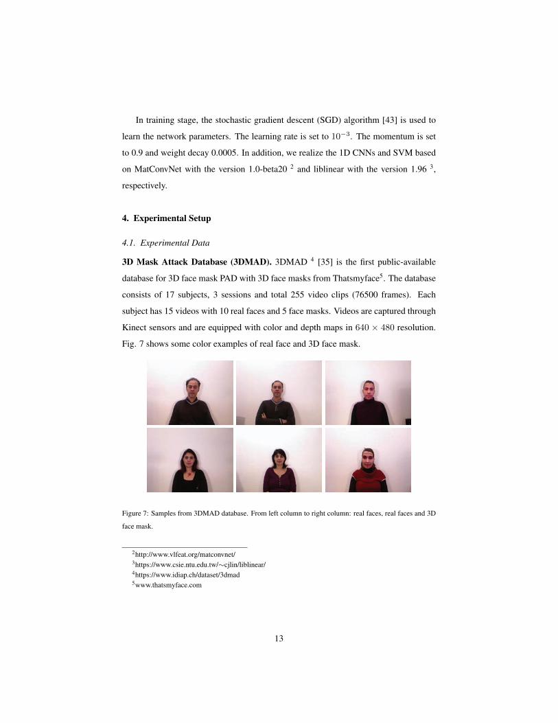
3D Mask Attack Database (3DMAD). 3DMAD 4 [35] is the first public-available

database for 3D face mask PAD with 3D face masks from Thatsmyface5. The database

consists of 17 subjects, 3 sessions and total 255 video clips (76500 frames). Each

subject has 15 videos with 10 real faces and 5 face masks. Videos are captured through

Kinect sensors and are equipped with color and depth maps in 640 × 480 resolution.

Fig. 7 shows some color examples of real face and 3D face mask.

learn the network parameters. The learning rate is set to 10−3. The momentum is set

to 0.9 and weight decay 0.0005. In addition, we realize the 1D CNNs and SVM based

on MatConvNet with the version 1.0-beta20 2 and liblinear with the version 1.96 3,

respectively.215

4. Experimental Setup

4.1. Experimental Data

3D Mask Attack Database (3DMAD). 3DMAD 4 [35] is the first public-available

database for 3D face mask PAD with 3D face masks from Thatsmyface5. The database

consists of 17 subjects, 3 sessions and total 255 video clips (76500 frames). Each220

subject has 15 videos with 10 real faces and 5 face masks. Videos are captured through

Kinect sensors and are equipped with color and depth maps in 640 × 480 resolution.

Fig. 7 shows some color examples of real face and 3D face mask.

Figure 7: Samples from 3DMAD database. From left column to right column: real faces, real faces and 3D

face mask.

HKBU-MARs V1. HKBU-MARs V1 6 [36] is a supplementary database for 3D face

2http://www.vlfeat.org/matconvnet/3https://www.csie.ntu.edu.tw/∼cjlin/liblinear/4https://www.idiap.ch/dataset/3dmad5www.thatsmyface.com6http://rds.comp.hkbu.edu.hk/mars/

13

Figure 7: Samples from 3DMAD database. From left column to right column: real faces, real faces and 3D

face mask.

2http://www.vlfeat.org/matconvnet/3https://www.csie.ntu.edu.tw/∼cjlin/liblinear/4https://www.idiap.ch/dataset/3dmad5www.thatsmyface.com

13

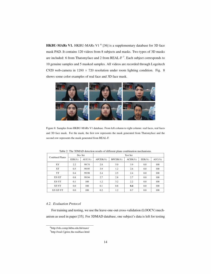
HKBU-MARs V1. HKBU-MARs V1 6 [36] is a supplementary database for 3D face

mask PAD. It contains 120 videos from 8 subjects and masks. Two types of 3D masks

are included: 6 from Thatsmyface and 2 from REAL-F 7. Each subject corresponds to

10 genuine samples and 5 masked samples. All videos are recorded through Logeitech

C920 web-camera in 1280 × 720 resolution under room lighting condition. Fig. 8

shows some color examples of real face and 3D face mask.

mask PAD. It contains 120 videos from 8 subjects and masks. Two types of 3D masks225

are included: 6 from Thatsmyface and 2 from REAL-F 7. Each subject corresponds to

10 genuine samples and 5 masked samples. All videos are recorded through Logeitech

C920 web-camera in 1280 × 720 resolution under room lighting condition. Fig. 8

shows some color examples of real face and 3D face mask.

Figure 8: Samples from HKBU-MARs V1 database. From left column to right column: real faces, real faces

and 3D face mask. For the mask, the first row represents the mask generated from Thatsmyface and the

second row represents the mask generated from REAL-F.

Table 2: The 3DMAD detection results of different plane combination mechanisms.

Combined PlanesDev Set Test Set

EER(%) AUC(%) APCER(%) BPCER(%) ACER(%) EER(%) AUC(%)

XY 2.2 99.74 2.8 5.0 3.9 0.0 100

XT 0.5 99.95 3.9 1.2 2.6 0.0 100

YT 0.4 99.98 2.4 2.5 2.4 0.0 100

XY-XT 0.8 99.94 2.7 2.8 2.7 0.0 100

XY-YT 0.1 100 1.2 3.2 2.2 0.0 100

XT-YT 0.0 100 0.1 0.8 0.4 0.0 100

XY-XT-YT 0.0 100 0.2 1.2 0.7 0.0 100

4.2. Evaluation Protocol230

For training and testing, we use the leave-one-out cross-validation (LOOCV) mech-

anism as used in paper [35]. For 3DMAD database, one subject’s data is left for testing

while the data of the remaining 16 subjects is divided into two subject-disjoint halves

7http://real-f.jp/en the-realface.html

14

Figure 8: Samples from HKBU-MARs V1 database. From left column to right column: real faces, real faces

and 3D face mask. For the mask, the first row represents the mask generated from Thatsmyface and the

second row represents the mask generated from REAL-F.

Table 2: The 3DMAD detection results of different plane combination mechanisms.

Combined PlanesDev Set Test Set


XY 2.2 99.74 2.8 5.0 3.9 0.0 100

XT 0.5 99.95 3.9 1.2 2.6 0.0 100

YT 0.4 99.98 2.4 2.5 2.4 0.0 100

XY-XT 0.8 99.94 2.7 2.8 2.7 0.0 100

XY-YT 0.1 100 1.2 3.2 2.2 0.0 100

XT-YT 0.0 100 0.1 0.8 0.4 0.0 100

XY-XT-YT 0.0 100 0.2 1.2 0.7 0.0 100

4.2. Evaluation Protocol

For training and testing, we use the leave-one-out cross-validation (LOOCV) mech-

anism as used in paper [35]. For 3DMAD database, one subject’s data is left for testing

6http://rds.comp.hkbu.edu.hk/mars/7http://real-f.jp/en the-realface.html

14

while the data of the remaining 16 subjects is divided into two subject-disjoint halves

as training and development sets in each fold of cross validations. However, for KBU-

MARs V1 database, we only use this database for inter-test as one person’s video data

is not published.

With performance evaluation, the results are reported in term of recently stan-

dardized ISO/IEC 30107-3 metrics [44]: Attack Presentation Classification Error Rate

(APCER) and Bona Fide Presentation Classification Error Rate (BPCER). It is noted

that the APCER and BPCER depend on the decision threshold estimated by Equal Er-

ror Rate (EER) on the development set. To compare the overall system performance

in a single value, the Average Classification Error Rate (ACER) is computed, which is

the average of the APCER and the BPCER [45]. To compare with existing works, we

also report the results of EER and Area Under Curve (AUC) on the test set.

5. Experimental Results and Discussion

In this part, the intensity histograms of different planes are firstly evaluated on the

detection performance. Then, various color spaces are analyzed for 3D face mask PAD.

Furthermore, we extract the intensity histograms from original face images and com-

pare the detection results with intrinsic images. After that, the inter-test experiments

are performed on HKBU-MARs V1 database. Finally, the performance of our method

is compared against the state-of-the-art approaches.

Table 3: The 3DMAD detection results of different color spaces.

Color SpaceDev Set Test Set


RGB 9.9 96.55 5.3 12.3 8.8 3.2 98.53

YCbCr 0.5 99.97 0.8 1.3 1.0 0.0 100

HSV 0.0 100 0.1 0.8 0.4 0.0 100

5.1. Three Orthogonal Planes

Table 2 illustrates the results of the intensity histograms extracted from different

planes and combined using different mechanisms. From the table, we can clearly find

that all averaged EERs and all averaged AUCs of test sets are 0.0% and 100%. This

15

means that our proposed method can accurately distinguish between real faces and 3D

masks by the decision threshold determined by the data set itself. However, when the

test set uses the threshold of the development set, the detection performance of the

algorithm in the test set will decrease. In addition, for combining different intensity

histograms, it is shown that simultaneously concatenating TOP histograms will not

improve the detection accuracy. We conjecture that the reason may lie in that the

feature dimension is too high for the classifier to overfit. Rather, when cascading the

intensity histograms extracted from XT and YT planes, our algorithm achieve the best

results with APCER=0.1%, BPCER=0.8% and ACER=0.4%. This reflects the fact that

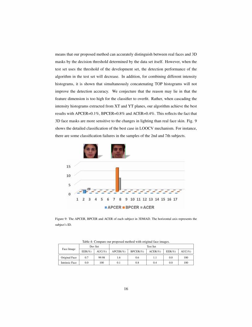
3D face masks are more sensitive to the changes in lighting than real face skin. Fig. 9

shows the detailed classification of the best case in LOOCV mechanism. For instance,

there are some classification failures in the samples of the 2nd and 7th subjects.

masks by the decision threshold determined by the data set itself. However, when the

test set uses the threshold of the development set, the detection performance of the

algorithm in the test set will decrease. In addition, for combining different intensity

histograms, it is shown that simultaneously concatenating TOP histograms will not260

improve the detection accuracy. We conjecture that the reason may lie in that the

feature dimension is too high for the classifier to overfit. Rather, when cascading the

intensity histograms extracted from XT and YT planes, our algorithm achieve the best

results with APCER=0.1%, BPCER=0.8% and ACER=0.4%. This reflects the fact that

3D face masks are more sensitive to the changes in lighting than real face skin. Fig. 9265

shows the detailed classification of the best case in LOOCV mechanism. For instance,

there are some classification failures in the samples of the 2nd and 7th subjects.

Figure 9: The APCER, BPCER and ACER of each subject in 3DMAD. The horizontal axis represents the

subject’s ID.

Table 4: Compare our proposed method with original face images.

Face ImageDev Set Test Set


Original Face 0.7 99.98 1.6 0.6 1.1 0.0 100

Intrinsic Face 0.0 100 0.1 0.8 0.4 0.0 100

16

Figure 9: The APCER, BPCER and ACER of each subject in 3DMAD. The horizontal axis represents the

subject’s ID.

Table 4: Compare our proposed method with original face images.

Face ImageDev Set Test Set


Original Face 0.7 99.98 1.6 0.6 1.1 0.0 100

Intrinsic Face 0.0 100 0.1 0.8 0.4 0.0 100

16

Table 5: The detection results of inter-test.

Face MaskTrained on 3DMAD Test on HKBU

APCER(%) BPCER(%) ACER(%) EER(%) AUC(%)

Thatsmyface 100 0 50 57.2 49.99

REAL-F 100 0 50 89.8 4.4

5.2. Different Color Spaces

Furthermore, we extract the histograms from different color spaces (i.e. RGB,

YCbCr and HSV), and compare the detection results in Table 3. The table shows

that the color is a very important clue for 3D face mask PAD. Compared to the RGB

color space, the YCbCr and HSV display color and brightness in different channels.

For instance, the HSV shows the brightness information in H channel and the color

information in S and V channels. When the intensity histograms are extracted from the

color channel and brightness channel respectively, the detection performance of our

algorithm can be significantly improved. It can be observed in Table 3 that the ACER

of HSV is 22 times lower than the ACER of the RGB color space.

5.3. Comparison with Original Face Image

In order to verify the validity of the proposed intrinsic image analysis, we extract

the intensity histograms from original face images in HSV color space and calculate

the intensity variational information also using 1D CNN. The comparison results are

shown in Table 4. When extracting the intensity histograms from original face images,

the EER of dev set and ACER of test set are 0.7% and 1.1%, respectively. Compared

the results of our proposed intrinsic image analysis based method, the ACER is reduced

by nearly three times. This shows that it is reasonable and effective to detect 3D face

mask in intrinsic image space.

5.4. Cross Database Evaluation

To gain insight into the generalization capabilities of our proposed detection method,

we conduct a cross-database evaluation. To be more specific, the countermeasure is

trained and tuned on 3DMAD and then tested on HKBU-MARs V1 database. The ob-

tained detection results are summarized in Table 5. During the experiment, the first 9

17

subjects in 3DMAD are used to train our algorithm, and the remaining 8 subjects are

used as the development set. When classifying according to the threshold of 3DMAD

database, all 3D face masks are detected incorrectly with APCER=100% and all real

faces are correctly classified with BPCER=0%. The reason may lie in that the materials

of face mask of these two databases are different. From these results, we conclude that

our proposed method is only for detecting the 3D face masks with specific material.

Table 6: Comparison between our proposed countermeasure and state-of-the-art methods on 3DMAD

database.

MethodsTest Set

ACER(%) EER(%) AUC(%)

MS-LBP [35]† - 5.2 98.65

fc-CNN [25]† - 3.2 98.36

LBP-TOP [29]† - 1.4 99.92

rPPG[36]† - 8.6 96.81

DCCTL [37] - 0.6 99.99

Pulse [15] 7.9 4.7 -

Our Method 0.4 0.0 100

† the results are reported in [37].

5.5. Comparison with the State of the Art

Table 6 gives a comparison with the state-of-the-art in 3D face mask PAD tech-

niques proposed in the literature. It can be seen that our proposed intrinsic image

analysis based method outperforms the-state-of-the-art algorithms on the EERs of de-

velopment set test set. Especially compared with the pulse detection based algorithms

[36, 15], the ACER of our proposed method is 0.4%, which is nearly 20 times better

than the ACER obtained by [15]. As aforementioned, the reason may lie in the pulse

detection based methods are sensitive to camera settings and light conditions. For LBP-

TOP [29] and DCCTL [37], their EERs are 1.4% and 0.6%, respectively. Even though

the performances are better than pulse detection based methods, they can be interfered

by the attacker’s head shake. Unfortunately, for 3D face mask PAD, there is only one

fully public database (i.e. 3DMAD) so far, which makes it difficult to fully verify the

effectiveness of our algorithm.

18

6. Conclusion

In this article, we addressed the problem of 3D face mask PAD from the viewpoint

of intrinsic image analysis. We designed a new feature for reflectance characteristic

description. Apart from that, we also introduced 1D CNN to extract intensity varia-

tion features. Extensive experiments on 3DMAD database showed excellent results.

However, deep features extracted from three orthogonal planes should have different

weights, but in our approach we simply concatenate them together. Therefore, we will

design a attention model to tackle this problem. For the generalization capability, we

think developing a 3D face mask PAD method with interoperability is big open issue,

which is far from the current state of the art. So we leave it to future work.

References

References

[1] D. Oberhaus, iphone x’s face id can be fooled with a 3d-printed mask,

https://motherboard.vice.com/en_us/article/qv3n77/

iphone-x-face-id-mask-spoof?utm_source=mbfb (Nov 2017).

[2] I. Chingovska, A. Anjos, S. Marcel, On the effectiveness of local binary patterns

in face anti-spoofing, in: Biometrics Special Interest Group, 2012, pp. 1–7.

[3] N. Erdogmus, S. Marcel, Spoofing in 2d face recognition with 3d masks and

anti-spoofing with kinect, in: IEEE Sixth International Conference on Biomet-

rics: Theory, Applications and Systems, 2013, pp. 1–6. doi:10.1109/BTAS.

2013.6712688.

[4] J. Maatta, A. Hadid, M. Pietikainen, Face spoofing detection from single images

using micro-texture analysis, in: International Joint Conference on Biometrics,

2011, pp. 1–7. doi:10.1109/IJCB.2011.6117510.

[5] Z. Boulkenafet, J. Komulainen, A. Hadid, Face anti-spoofing based on color tex-

ture analysis, in: IEEE International Conference on Image Processing, 2015, pp.

2636–2640. doi:10.1109/ICIP.2015.7351280.

19

https://motherboard.vice.com/en_us/article/qv3n77/iphone-x-face-id-mask-spoof?utm_source=mbfb

https://motherboard.vice.com/en_us/article/qv3n77/iphone-x-face-id-mask-spoof?utm_source=mbfb

http://dx.doi.org/10.1109/BTAS.2013.6712688


http://dx.doi.org/10.1109/IJCB.2011.6117510

http://dx.doi.org/10.1109/ICIP.2015.7351280

[6] G. Pan, L. Sun, Z. Wu, S. Lao, Eyeblink-based anti-spoofing in face recogni-

tion from a generic webcamera, in: IEEE International Conference on Computer

Vision, 2007, pp. 1–8. doi:10.1109/ICCV.2007.4409068.

[7] Y. Li, X. Tan, An anti-photo spoof method in face recognition based on the anal-

ysis of fourier spectra with sparse logistic regression, in: Chinese Conference on

Pattern Recognition, 2009, pp. 1–5. doi:10.1109/CCPR.2009.5344092.

[8] Z. Zhang, J. Yan, S. Liu, Z. Lei, D. Yi, S. Z. Li, A face antispoofing database with

diverse attacks, in: International Conference on Biometrics, 2012, pp. 26–31.

doi:10.1109/ICB.2012.6199754.

[9] X. Tan, Y. Li, J. Liu, L. Jiang, Face liveness detection from a single image with

sparse low rank bilinear discriminative model, in: European Conference on Com-

puter Vision, 2010, pp. 504–517. doi:10.1007/978-3-642-15567-3_

37.

[10] H. Li, S. Wang, A. C. Kot, Face spoofing detection with image quality regression,

in: International Conference on Image Processing Theory Tools and Applications,

2016, pp. 1–6. doi:10.1109/IPTA.2016.7821027.

[11] I. Pavlidis, P. Symosek, The imaging issue in an automatic face/disguise detection

system, in: IEEE Workshop on Computer Vision Beyond the Visible Spectrum:

Methods and Applications, 2000, pp. 15–24. doi:10.1109/CVBVS.2000.

855246.

[12] Z. Zhang, D. Yi, Z. Lei, S. Z. Li, Face liveness detection by learning multispectral

reflectance distributions, in: IEEE International Conference on Automatic Face

and Gesture Recognition and Workshops, 2011, pp. 436–441. doi:10.1109/

FG.2011.5771438.

[13] L. Li, P. L. Correia, A. Hadid, Face recognition under spoofing attacks: coun-

termeasures and research directions, IET Biometrics 7 (1) (2018) 3–14. doi:

10.1049/iet-bmt.2017.0089.

20

http://dx.doi.org/10.1109/ICCV.2007.4409068

http://dx.doi.org/10.1109/CCPR.2009.5344092

http://dx.doi.org/10.1109/ICB.2012.6199754

http://dx.doi.org/10.1007/978-3-642-15567-3_37

http://dx.doi.org/10.1007/978-3-642-15567-3_37

http://dx.doi.org/10.1109/IPTA.2016.7821027

http://dx.doi.org/10.1109/CVBVS.2000.855246

http://dx.doi.org/10.1109/CVBVS.2000.855246

http://dx.doi.org/10.1109/FG.2011.5771438

http://dx.doi.org/10.1109/FG.2011.5771438

http://dx.doi.org/10.1049/iet-bmt.2017.0089

http://dx.doi.org/10.1049/iet-bmt.2017.0089

[14] Y. Liu, A. Jourabloo, X. Liu, Learning deep models for face anti-spoofing: Binary

or auxiliary supervision, in: IEEE Conference on Computer Vision and Pattern

Recognition, 2018, pp. 389–398.

[15] X. Li, J. Komulainen, G. Zhao, P. C. Yuen, M. Pietikainen, Generalized face

anti-spoofing by detecting pulse from face videos, in: International Conference

on Pattern Recognition, 2017, pp. 4244–4249. doi:10.1109/ICPR.2016.

7900300.

[16] Y. Ma, X. Feng, X. Jiang, Z. Xia, J. Peng, Intrinsic image decomposition: A com-

prehensive review, in: Image and Graphics, Springer International Publishing,

Cham, 2017, pp. 626–638.

[17] X. Jiang, A. J. Schofield, J. L. Wyatt, Correlation-based intrinsic image extraction

from a single image, in: European Conference on Computer Vision, Springer,

2010, pp. 58–71.

[18] A. Agarwal, R. Singh, M. Vatsa, Face anti-spoofing using haralick features, in:

IEEE International Conference on Biometrics Theory, Applications and Systems,

2016, pp. 1–6. doi:10.1109/BTAS.2016.7791171.

[19] K. Patel, H. Han, A. K. Jain, Secure face unlock: Spoof detection on smartphones,

IEEE transactions on information forensics and security 11 (10) (2016) 2268–

2283.

[20] Z. Boulkenafet, J. Komulainen, A. Hadid, Face spoofing detection using colour

texture analysis, IEEE Transactions on Information Forensics and Security 11 (8)

(2016) 1818–1830. doi:10.1109/TIFS.2016.2555286.

[21] D. Wen, H. Han, A. K. Jain, Face spoof detection with image distortion analysis,

IEEE Transactions on Information Forensics and Security 10 (4) (2015) 746–761.

doi:10.1109/TIFS.2015.2400395.

[22] J. Yang, Z. Lei, S. Z. Li, Learn convolutional neural network for face anti-

spoofing, Computing Research Repository abs/1408.5601 (2014) 373–384.

21

http://dx.doi.org/10.1109/ICPR.2016.7900300

http://dx.doi.org/10.1109/ICPR.2016.7900300


http://dx.doi.org/10.1109/TIFS.2016.2555286


[23] L. Li, X. Feng, Z. Boulkenafet, Z. Xia, M. Li, A. Hadid, An original face anti-

spoofing approach using partial convolutional neural network, in: International

Conference on Image Processing Theory Tools and Applications, 2016, pp. 1–6.

doi:10.1109/IPTA.2016.7821013.

[24] L. Li, X. Feng, X. Jiang, Z. Xia, A. Hadid, Face anti-spoofing via deep local

binary patterns, in: IEEE International Conference on Image Processing, 2018,

pp. 101–105. doi:10.1109/ICIP.2017.8296251.

[25] L. Sun, G. Pan, Z. Wu, S. Lao, Blinking-based live face detection using condi-

tional random fields, in: Advances in Biometrics, Springer Berlin Heidelberg,

Berlin, Heidelberg, 2007, pp. 252–260.

[26] A. Anjos, S. Marcel, Counter-measures to photo attacks in face recognition: A

public database and a baseline, in: International Joint Conference on Biometrics,

2011, pp. 1–7. doi:10.1109/IJCB.2011.6117503.

[27] B. Zhang, Y. Gao, S. Zhao, J. Liu, Local derivative pattern versus local binary

pattern: Face recognition with high-order local pattern descriptor, IEEE Trans-

actions on Image Processing 19 (2) (2010) 533–544. doi:10.1109/TIP.

2009.2035882.

[28] W. Bao, H. Li, N. Li, W. Jiang, A liveness detection method for face recogni-

tion based on optical flow field, in: International Conference on Image Analy-

sis and Signal Processing, 2009, pp. 233–236. doi:10.1109/IASP.2009.

5054589.

[29] T. d. Freitas Pereira, J. Komulainen, A. Anjos, J. M. De Martino, A. Ha-

did, M. Pietikainen, S. Marcel, Face liveness detection using dynamic texture,

EURASIP Journal on Image and Video Processing 2014 (1) (2014) 2. doi:

10.1186/1687-5281-2014-2.

[30] Z. Xu, S. Li, W. Deng, Learning temporal features using lstm-cnn architecture

for face anti-spoofing, in: Asian Conference on Pattern Recognition, 2015, pp.

141–145. doi:10.1109/ACPR.2015.7486482.

22

http://dx.doi.org/10.1109/IPTA.2016.7821013


http://dx.doi.org/10.1109/IJCB.2011.6117503

http://dx.doi.org/10.1109/TIP.2009.2035882

http://dx.doi.org/10.1109/TIP.2009.2035882

http://dx.doi.org/10.1109/IASP.2009.5054589

http://dx.doi.org/10.1109/IASP.2009.5054589

http://dx.doi.org/10.1186/1687-5281-2014-2

http://dx.doi.org/10.1186/1687-5281-2014-2

http://dx.doi.org/10.1109/ACPR.2015.7486482

[31] H. Li, P. He, S. Wang, A. Rocha, X. Jiang, A. C. Kot, Learning generalized deep

feature representation for face anti-spoofing, IEEE Transactions on Information

Forensics and Security (2018) 1–14doi:10.1109/TIFS.2018.2825949.

[32] S. Kim, Y. Ban, S. Lee, Face liveness detection using a light field camera, Sensors

14 (12) (2014) 22471–22499. doi:10.3390/s141222471.

[33] Z. Ji, H. Zhu, Q. Wang, Lfhog: A discriminative descriptor for live face detection

from light field image, in: IEEE International Conference on Image Processing,

2016, pp. 1474–1478. doi:10.1109/ICIP.2016.7532603.

[34] F. P. A. Sepas-Moghaddam, P. Correia, Light field local binary patterns descrip-

tion for face recognition, in: IEEE International Conference on Image Processing,

2017, pp. 3815–3819. doi:10.1109/ICIP.2017.8296996.

[35] N. Erdogmus, S. Marcel, Spoofing face recognition with 3d masks, IEEE trans-

actions on information forensics and security 9 (7) (2014) 1084–1097.

[36] S. Liu, P. C. Yuen, S. Zhang, G. Zhao, 3d mask face anti-spoofing with remote

photoplethysmography, in: European Conference on Computer Vision, Springer,

2016, pp. 85–100.

[37] R. Shao, X. Lan, P. C. Yuen, Deep convolutional dynamic texture learning with

adaptive channel-discriminability for 3d mask face anti-spoofing, in: IEEE Inter-

national Joint Conference on Biometrics (IJCB), IEEE, 2017, pp. 748–755.

[38] K. Simonyan, A. Zisserman, Very deep convolutional networks for large-scale

image recognition, Computing Research Repository abs/1409.1556. arXiv:

1409.1556.

[39] K. Patel, H. Han, A. K. Jain, Cross-database face antispoofing with robust feature

representation, in: Chinese Conference on Biometric Recognition, 2016, pp. 611–

619. doi:10.1007/978-3-319-46654-5_67.

[40] M. S. M. Sajjadi, B. Scholkopf, ichael Hirsch, Enhancenet: Single image super-

resolution through automated texture synthesis, CoRR abs/1612.07919. arXiv:

23


http://dx.doi.org/10.3390/s141222471



http://arxiv.org/abs/1409.1556


http://dx.doi.org/10.1007/978-3-319-46654-5_67




1612.07919.

URL http://arxiv.org/abs/1612.07919

[41] X. Glorot, A. Bordes, Y. Bengio, X. Glorot, A. Bordes, Y. Bengio, Deep sparse

rectifier neural networks, in: International Conference on Artificial Intelligence

and Statistics, 2011, pp. 315–323.

[42] O. M. Parkhi, A. Vedaldi, A. Zisserman, Deep face recognition, in: British Ma-

chine Vision Conference, 2015, pp. 1–12.

[43] L. Bottou, Large-scale machine learning with stochastic gradient descent, in: Pro-

ceedings of COMPSTAT’2010, Physica-Verlag HD, 2010, pp. 177–186. doi:

10.1007/978-3-7908-2604-3_16.

[44] Iso/iec jtc 1/sc 37 biometrics. information technology - biometric presentation

attack detection - part 1: Framework, Tech. rep., International Organization for

Standardization (2016).

[45] Z. Boulkenafet, J. Komulainen, L. Li, X. Feng, A. Hadid, Oulu-npu: A mobile

face presentation attack database with real-world variations, in: IEEE Interna-

tional Conference on Automatic Face & Gesture Recognition (FG 2017), IEEE,

2017, pp. 612–618.

24



http://dx.doi.org/10.1007/978-3-7908-2604-3_16

http://dx.doi.org/10.1007/978-3-7908-2604-3_16

Date post:	28-May-2020
Category:	Documents
Upload:	others
View:	18 times
Download:	0 times

3D Face Mask Presentation Attack Detection Based on ... · 3D Face Mask Presentation Attack...

Documents