Int. J. MAr. Sci. Eng., 4(1), 37-46, Winter & Spring 2014

ISSN 2251-6743

© IAU

3D Finite element modeling for Dynamic Behavior Evaluation of

Marin Risers Due to VIV and Internal Flow

* M. Ghodsi Hassanabad; A. Fardad

Marine industries group, Science and research branch, Islamic Azad University, Tehran, Iran

Received 17 January 2014; Revised 28 March 2014; Accepted 20 April 2014

ABSTRACT: The complete 3D nonlinear dynamic problem of extensible, flexible risers conveying fluid is

considered. For describing the dynamics of the system, the Newtonian derivation procedure is followed. The velocity

field inside the pipe formulated using hydrostatic and Bernoulli equations. The hydrodynamic effects of external

fluids are taken into consideration through the nonlinear drag forces in various time steps and the added inertia due to

the hydrodynamic mass. Following the Newtonian derivation, the dynamics of the pipes element with effects of

internal fluid are considered separately and the final governing set is derived by combining the equations of inertia

equilibrium. The study focuses specifically on the effect of the inner flow to the global dynamics of the riser. This

task is accomplished using time domain teachings and the Finite Element method is used as a powerful numerical

method. Moreover the Euler-Bernoulli beam theory is used response to model the dynamic behavior of the flexible

risers.

Keywords: risers, inner flow, dynamic response, Finite Element Method (FEM)

INTRODUCTION

1 The dynamic behavior of cylindrical pipes with axial

flow has been extensively investigation in the past

(Paidoussis, 1998; Paidoussis, 2001).There is an

enormous amount of works reported in the literature

that treat a bulk of important engineering application.

An interesting subject in this context is the

application of flexible pipes that transport fluids,

especially when they operate in a wet environment

and they are subjected to external motions and

hydrodynamic forces. (Paidoussis, 2005)

Indicative examples of studies on the dynamics of

flexible Risers transporting fluid are those due to

(Misra, et al, 1988; Jain and Jayaraman, 1990;

Dupuis and Rousselet, 1992; Semler, et al, 1994;

Petrakis and Karahalios, 1997; Qiao et al, 2006; Lin

et al, 2007). The investigation concerns mainly 2D

formulation, while there are also studies that examine

problems in 3D, such as the work reported by

(Taniguchi et al, 2007) who investigated the out-of-

plane vibrations of flexible risers due to pulsating

flow and (Chai and Varyani, 2006) who presented a

general absolute coordinate formulation for the 3D

analysis of flexible pipe structure including the effect

of internal flow. The authors used a similar line of

approach adopted by (Paulling and Webster, 1986).

Recently, (Wadham-Gagnon, 2007) developed the

*Corresponding Author Email: m.ghodsi.h@gmail.com

nonlinear equation of 3D motion for unrestrained and

restrained cantilevered pipes conveying fluid. For the

unrestrained pipes, the equation of motions where

derived by assuming that the fluid is incompressible,

the flow is of constant velocity and the pipe behaves

as a nonlinear Euler-Bernoulli beam. Moreover, the

strain of the pipe was considered small while the

rotary inertia and the shear deformation were

neglected.

Typically, marine risers or free span pipe lines are

lengthy structures, subjected to externally imposed

excitations of various amplitudes and frequencies and

they are characterized by a relatively small equivalent

elasticity 𝐸𝐴

𝐿 due to their large length. In addition,

instability phenomena are difficult to be detected due

to the drastic contribution of drag forces.

Furthermore, the treatment of the problem in tow

dimensions is admittedly a short approximation as

these structure can be subjected to high frequency

cycling motions due to the externally imposed

excitations that originate from the behavior is

primarily governed by the imposed motions which

are normally applied at one end. Never the less, it is

very interesting to investigate the details of the 3D

dynamic of the associated nonlinear system under the

combined contribution of both sources of excitation,

namely external motions and internal flow. (Lecunff

and Biolley, 2005; Chatjigeorgiou and Damy, 2007)

M. Ghodsi Hassanabad and A. Fardad

38

Most of the studies on the dynamic of risers, at least

at they reviewed by (Chakrabarti and Frampton,

1982; Jain, 1994; Patel and Seyed, 1995) omit the

contribution of the internal flow. Moreover, with

regard to the works that consider the effect of the

fluid's velocity inside the pipe, it appears that special

attention is given to 2D formulation. Relevant

examples are the works of (Wu and Lou, 1991; Bar-

Avi, 2000; Chucheepsakul et al, 2003; kuiper et al,

2004; Chatjigergiou and Mavrakos, 2005;

Kaewunruen et al, 2005; Kupier and Metrikine, 2005;

Monprapussorn et al, 2007; Kuiper et al, 2008).

There are also studies special effects induced by

internal flow such as Vortex-induced-vibration or

Whipping phenomena. (Bordalo et al, 2008)

The present paper is dedicated to the formulation and

the solution of the complete 3D dynamic problem of

a flexible riser including the effect of the internal

flow. Effort has been made in developing a generic

formulation that could describe the dynamics of

general shapes of flexible risers or free span

pipelines. The work extends the research of the

present author on nonlinear dynamics of flexible

risers using an efficient finite element methods.

(Chatjigeorgiou et al, 2008) This is achieved by

extending the existing 2D formulation to 3D and

incorporating the internal flow.

The dynamic problem is also treated in the time

domain. The main goal in this context is the

derivation of the transfer functions of all dynamic

components, both in-plane and out-of-plane, that

influence the dynamics of the structures. The results

from the solution in the time domain is of paramount

importance as the transfer functions of the concerned

variables can easily demonstrate the details of the

dynamic behavior of the structure subjected to the

effect of the internal flow and the impacts of forced

excitations, while in addition this can be done with a

very descriptive way.

MATERIALS AND METHODS

Mathematical formulation and governing differential

equations

In this section the mathematical formulations for a

vertical pin-end beam subjected to the varying

tensions to the top tensions and the internal flow

effects and the impacts of hydrodynamic forced due

to the effects of the external fluid are explained.

In beams with high aspect ratio such as riser pipes,

Euler-Bernoulli beam theory can be used to model the

dynamics, because the transverse shear can be

neglected. When the diameter or width of the cross-

section is small compared to the length of the beam, it

can be considered that the planes perpendicular of the

axis remain plane and perpendicular to the axis after

deformation. (HueraHuarte, 2006)

The system of dynamic equilibrium is formulated

under the following assumptions: (i) the flow inside

the pipe is inviscous, incompressible and irrotational;

(ii) the pipe behaves as a nonlinear Euler-Bernoulli

beam; (iii) the centerline of the pipe is extensible

obeying to a liner stress-strain relations; (iv) shear,

bending and torsion effects are incorporated in to the

mathematical model but the final equations are solved

omitting torsion; (v) the ends of the pipe are pinned;

(vi) planar surfaces orthogonal to the axis of the

beam, remain planar and orthogonal to the axis after

the deformation.

A cartesian reference with its origin at the bottom of

the riser has been used, in which the X axis is parallel

to the external flow velocity, Z coincides with the

vertical axis of the riser in its undeflected

configuration and the Y is perpendicular to both. u(z,

t), v(z, t) and w(z, t) are defined as the time variant

in-line, cross-flow and the axial motions respectively.

With these set of displacements a point in the

centerline of the beam can be spatially described.

Combinations of translations and rotations around the

beam axis describe states of torsion, and the states of

bending are described by displacements and rotations

around the two axes contained in the plane

perpendicular to the beam axis. Because the riser was

attached to the supporting structures at its ends with

universal joints, torsion motions were avoided, but

the fact that the riser model was free to move in-line

and cross-flow at the same time, meant that small

twisting motions were inevitable. Moreover when the

first derivative in space of the transverse motions is

small 𝜕𝑢

𝜕𝑧≈ 0 and

𝜕𝑣

𝜕𝑧≈ 0 , as in the case presented

here, the non-linear terms in the stress equations

disappear and both transverse and axial motions

become uncoupled. (Reddy, 1993) and (Reddy,

2005).

Therefore, in problems involving small displacement

the motions in the planes XZ and YZ can be treated

independently.

Equation for the transverse motion (X or Y

directions)

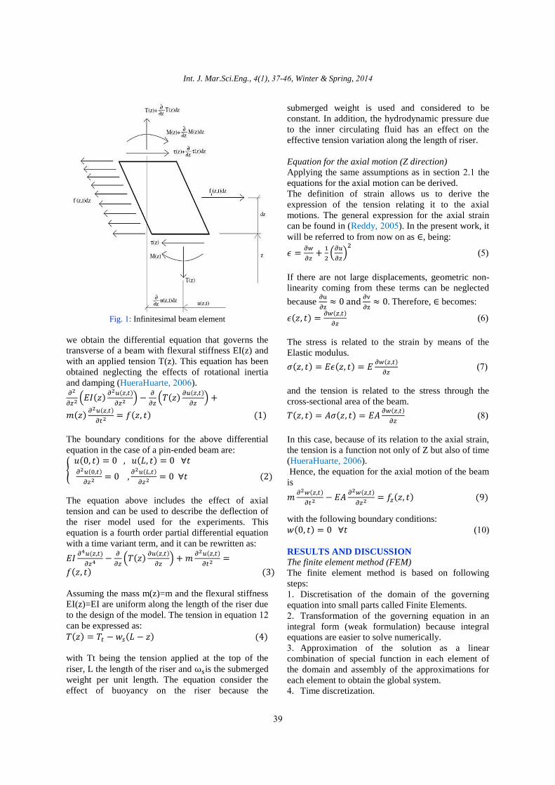
The transverse deformation of a generic beam can be

described with a fourth order differential equation

which can be derived by applying force and

momentum equilibrium to an infinitesimal section of

the beam, see the free-body diagram in Figure (1).

The formulation can be similarly applied to any of the

tow transverse directions, X or Y. where f is the

external fluid force, fi is the inertia force and τ is the

shear force, all referred to one of the transverse

directions, X or Y.

Int. J. Mar.Sci.Eng., 4(1), 37-46, Winter & Spring, 2014

39

Fig. 1: Infinitesimal beam element

we obtain the differential equation that governs the

transverse of a beam with flexural stiffness EI(z) and

with an applied tension T(z). This equation has been

obtained neglecting the effects of rotational inertia

and damping (HueraHuarte, 2006). 𝜕2

𝜕𝑧2 (𝐸𝐼(𝑧)𝜕2𝑢(𝑧,𝑡)

𝜕𝑧2 ) −𝜕

𝜕𝑧(𝑇(𝑧)

𝜕𝑢(𝑧,𝑡)

𝜕𝑧) +

𝑚(𝑧)𝜕2𝑢(𝑧,𝑡)

𝜕𝑡2 = 𝑓(𝑧, 𝑡) (1)

The boundary conditions for the above differential

equation in the case of a pin-ended beam are:

{ 𝑢(0, 𝑡) = 0 , 𝑢(𝐿, 𝑡) = 0 ∀𝑡 𝜕2𝑢(0,𝑡)

𝜕𝑧2 = 0 ,𝜕2𝑢(𝐿,𝑡)

𝜕𝑧2 = 0 ∀𝑡 (2)

The equation above includes the effect of axial

tension and can be used to describe the deflection of

the riser model used for the experiments. This

equation is a fourth order partial differential equation

with a time variant term, and it can be rewritten as:

𝐸𝐼𝜕4𝑢(𝑧,𝑡)

𝜕𝑧4 −𝜕

𝜕𝑧(𝑇(𝑧)

𝜕𝑢(𝑧,𝑡)

𝜕𝑧) + 𝑚

𝜕2𝑢(𝑧,𝑡)

𝜕𝑡2 =

𝑓(𝑧, 𝑡) (3)

Assuming the mass m(z)=m and the flexural stiffness

EI(z)=EI are uniform along the length of the riser due

to the design of the model. The tension in equation 12

can be expressed as:

𝑇(𝑧) = 𝑇𝑡 − 𝑤𝑠(𝐿 − 𝑧) (4)

with Tt being the tension applied at the top of the

riser, L the length of the riser and ωsis the submerged

weight per unit length. The equation consider the

effect of buoyancy on the riser because the

submerged weight is used and considered to be

constant. In addition, the hydrodynamic pressure due

to the inner circulating fluid has an effect on the

effective tension variation along the length of riser.

Equation for the axial motion (Z direction)

Applying the same assumptions as in section 2.1 the

equations for the axial motion can be derived.

The definition of strain allows us to derive the

expression of the tension relating it to the axial

motions. The general expression for the axial strain

can be found in (Reddy, 2005). In the present work, it

will be referred to from now on as ∈, being:

𝜖 =𝜕𝑤

𝜕𝑧+

1

2(

𝜕𝑢

𝜕𝑧)

2

(5)

If there are not large displacements, geometric non-

linearity coming from these terms can be neglected

because ∂u

∂z≈ 0 and

∂v

∂z≈ 0. Therefore, ∈ becomes:

𝜖(𝑧, 𝑡) =𝜕𝑤(𝑧,𝑡)

𝜕𝑧 (6)

The stress is related to the strain by means of the

Elastic modulus.

𝜎(𝑧, 𝑡) = 𝐸𝜖(𝑧, 𝑡) = 𝐸𝜕𝑤(𝑧,𝑡)

𝜕𝑧 (7)

and the tension is related to the stress through the

cross-sectional area of the beam.

𝑇(𝑧, 𝑡) = 𝐴𝜎(𝑧, 𝑡) = 𝐸𝐴𝜕𝑤(𝑧,𝑡)

𝜕𝑧 (8)

In this case, because of its relation to the axial strain,

the tension is a function not only of Z but also of time

(HueraHuarte, 2006).

Hence, the equation for the axial motion of the beam

is

𝑚𝜕2𝑤(𝑧,𝑡)

𝜕𝑡2 − 𝐸𝐴𝜕2𝑤(𝑧,𝑡)

𝜕𝑧2 = 𝑓𝑧(𝑧, 𝑡) (9)

with the following boundary conditions:

𝑤(0, 𝑡) = 0 ∀𝑡 (10)

RESULTS AND DISCUSSION

The finite element method (FEM)

The finite element method is based on following

steps:

1. Discretisation of the domain of the governing

equation into small parts called Finite Elements.

2. Transformation of the governing equation in an

integral form (weak formulation) because integral

equations are easier to solve numerically.

3. Approximation of the solution as a linear

combination of special function in each element of

the domain and assembly of the approximations for

each element to obtain the global system.

4. Time discretization.

3D Finite element modeling for Dynamic Behavior Evaluation of Marin Risers

40

After these steps the initial partial differential

equation are transformed into an algebraic system and

much easier to solve.

Discretization of the riser

The flexible riser is idealized as a one-dimensional

domain with the neutral axis of the structure. A mesh

formed by one-dimensional elements can be used, in

which a generic finite element Ωe consists of tow

nodes, and is referred to, as

Ω𝑒 = [𝑧1𝑒 , 𝑧2

𝑒] (11)

with the length of element defined as

ℎ𝑒 = 𝑧2𝑒−𝑧1

𝑒 (12)

being z1e and z2

e the global coordinate of the finite

element at the first and the second node respectively.

The number of element, ne is

𝑛𝑒 =𝐿

ℎ𝑒 (13)

and the number of nodes

𝑛 = 𝑛𝑒 + 1 (14)

The solution of the equation 3 in each element will be

approximated with

𝑢𝑒(𝑧, 𝑡) ≃ ue(t)Ψ𝑒(𝑧) = ∑ 𝑢𝑗𝑒

𝑁𝑡

𝑗=1

(𝑡)𝜓𝑗𝑒(𝑧) (15)

𝜐𝑒(𝑧, 𝑡) ≃ 𝑉𝑒(𝑡)Ψ𝑒(𝑧) = ∑ 𝜐𝑗𝑒𝑁𝑡

𝑗=1 (𝑡)𝜓𝑗𝑒(𝑧) (16)

𝑤𝑒(𝑧, 𝑡) ≃ 𝑊𝑒(𝑡)𝐿𝑒(𝑧) = ∑ 𝑤𝑗𝑒

𝑁𝑎

𝑗=1

(𝑡)𝑙𝑗𝑒(𝑧) (17)

According to this approximation, the transverse

deflections of the riser in each finite element,

depending on time and position, ue(z, t) and ve(z, t),

are the linear combination of the time dependent

deflections at the node j that is uje(t) and vj

e(t),

multiplied by spatial approximation functions ψje(t),

according to each of the Nt degrees of freedom in

both nodes of the finite element. The same applies of

the axial motions ωje(t) with the spatial functions

lje(t)s and Na degree of freedom. The approximation

function are known as shape functions.

The bending states result from motions and rotations

(first derivatives in space of the displacements), so

the finite elements for the transverse case must be

able to represent tow degrees of freedom at each

node, and it implies Nt=4 degrees of freedom. The

rotations, around the axis of the pipe are neglected,

and this result in only one degree of freedom at each

nodes of the finite element associated to the axial

displacements with Na=2 degree of freedom.

Weak formulation

The need for an integral form of equation 3 comes

from the fact that if equations 15 and 16 are

substituted in the governing equation 3, it is possible

that the resultant system would not always have the

required number of linearly independent algebraic

equations needed to find the coefficients Uje(t),

Vje(t), that represent the solution of our system at

each node. The same could happen with Wje(t) when

substituting eq.17 in the axial equation of motion,

eq.9. A way to obtain the correct number of linearly

independent equations is to final the integral weak

formulation of the governing equation (Reddy, 1993).

A weight function υ(z) is used for the purpose,

multiplying the governing equation and integrating

along the element to find the weak form of the

differential equation.

Weak formulation for transverse equations of motion

(X or Y direction)

In the case of the transverse equations of motion the

procedure is valid for both the equations modeling the

motion in the XZ and YX planes. Introducing the

weight function υ(z) into equation 3,

∫ 𝜗(𝑧) [𝐸𝐼𝜕4𝑢(𝑧,𝑡)

𝜕𝑧4 −𝜕

𝜕𝑧(𝑇(𝑧)

𝜕𝑢(𝑧,𝑡)

𝜕𝑧) + 𝑚

𝜕2𝑢(𝑧,𝑡)

𝜕𝑡2 −𝑧2

𝑒

𝑧1𝑒

𝑓(𝑧, 𝑡)] 𝑑𝑧 = 0 (18)

Integration by parts once in the second order term,

and twice in the fourth order one, allows to obtain the

weak formulation of the differential equation as

fallow:

∫ [𝑇(𝑧)𝜕𝜗

𝜕𝑧

𝜕𝑢

𝜕𝑧+ 𝐸𝐼

𝜕2𝜗

𝜕𝑧2

𝜕2𝑢

𝜕𝑧2 + 𝑚𝑤𝜕2𝑢

𝜕𝑡2 − 𝑤𝑓] 𝑑𝑧 −𝑧2

𝑒

𝑧1𝑒

𝑄1𝜗( 𝑧1𝑒) − 𝑄2𝜗(𝑧2

𝑒) − 𝑄1 (𝜕𝜗

𝜕𝑧(𝑧1

𝑒)) −

𝑄2 (𝜕𝜗

𝜕𝑧(𝑧2

𝑒)) = 0 (19)

Because it is a fourth order differential equation we

have two primary variables u(z,t) and ∂u

∂z(z, t). That

means each nodes has associated with it two degrees

of freedom, one for each primary variable on the

other hand, the secondary variables are:

𝑄1(𝑡) = [−𝑇(𝑧)𝜕𝑢

𝜕𝑧+

𝜕

𝜕𝑧(𝐸𝐼

𝜕2𝑢

𝜕𝑧2)]𝑧=𝑧1

𝑒 (20)

𝑄2(𝑡) = − [−𝑇(𝑧)𝜕𝑢

𝜕𝑧+

𝜕

𝜕𝑧(𝐸𝐼

𝜕2𝑢

𝜕𝑧2)]𝑧=𝑧2

𝑒 (21)

𝑄1̅(𝑡) = 𝐸𝐼𝜕2𝑢

𝜕𝑧2|𝑧=𝑧1

𝑒 (22)

𝑄2̅(𝑡) = 𝐸𝐼𝜕2𝑢

𝜕𝑧2|𝑧=𝑧2

𝑒 (23)

Where the first ones represent shear forces and the

second ones bending moments. equation 24 results in

Int. J. Mar. Sci. Eng., 4(1), 37-46, Winter & Spring, 2014

41

a system of algebraic equations that gives the

approximate solution of 3 in the generic element Ωe.

It is the algebraic equation for both transverse

motions, either X or Y. It can be expressed in matrix

form as:

𝐾𝑒𝑈𝑒 + 𝑀𝑒�̈�𝑒 = 𝐹𝑥𝑒 + 𝑄𝑥

𝑒 In-line (24)

𝐾𝑒𝑉𝑒 + 𝑀𝑒�̈�𝑒 = 𝐹𝑦𝑒 + 𝑄𝑦

𝑒 Cross-flow (25)

where the vectors Ue and Ve gives the displacements

along the axis of the cylinder in the transverse

directions. The matrices are [4*4] because there are

two nodes and at each of them, two degrees of

freedom. Note that the displacements victor Ue is

formed by ui and - ∂u

∂z at each node, then its

components are Ue=[u1 u2 u3 u4]T. u1is the

displacement at the first node (Z1e), u2 = −

∂u

∂z is the

rotation in the first node. u3is the displacement at the

second node (Z2e) and u4 = −

∂u

∂z the rotation at the

second node. Ke is the stiffness matrix, Me is the

consistent mass matrix Fe is the transverse nodal

forces vector, and finally Qe is the secondary

variables vector. The reader must notice that Ke and

Me are valid for any of the two transverse directions,

X or Y. They are both symmetric and calculated as

follows,

𝐾𝑒 = 𝐾𝑒1+𝐾𝑒2

(26)

𝐾𝑒 = [𝐾𝑎

𝑒 𝐾𝑏𝑒

𝐾𝑐𝑒 𝐾𝑑

𝑒] (27)

where

𝐾𝑎𝑒 = [

𝐾11 𝐾12

𝐾21 𝐾22] 𝐾𝑏

𝑒 = [𝐾13 𝐾14

𝐾23 𝐾24] 𝐾𝑐

𝑒 =

[𝐾31 𝐾32

𝐾41 𝐾42] 𝐾𝑑

𝑒 = [𝐾33 𝐾34

𝐾43 𝐾44] (28)

taking into account that the same nomenclature is

followed for the mass matrix Me.

Weak formulation for axial equations of motion (Z

direction) The procedure of the case of the axial equation of

motion is the same. The weight functions are

introduced in equation follow multiplying all its

terms and then the integration is developed.

∫ 𝜗(𝑧) [𝐸𝐼𝜕4𝑢(𝑧,𝑡)

𝜕𝑧4 −𝜕

𝜕𝑧(𝑇(𝑧)

𝜕𝑢(𝑧,𝑡)

𝜕𝑧) + 𝑚

𝜕2𝑢(𝑧,𝑡)

𝜕𝑡2 −𝑧2

𝑒

𝑧1𝑒

𝑓(𝑧, 𝑡)] 𝑑𝑧 = 0 (29)

Integration by parts once in the second order term,

and twice in the fourth order one, allows to obtain the

weak formulation of the differential equation.

∫ [𝑇(𝑧)𝜕𝜗

𝜕𝑧

𝜕𝑢

𝜕𝑧+ 𝐸𝐼

𝜕2𝜗

𝜕𝑧2

𝜕2𝑢

𝜕𝑧2 + 𝑚𝑤𝜕2𝑢

𝜕𝑡2 − 𝑤𝑓] 𝑑𝑧 −𝑧2

𝑒

𝑧1𝑒

𝑄1𝜗( 𝑧1𝑒) − 𝑄2𝜗(𝑧2

𝑒) − 𝑄1 (𝜕𝜗

𝜕𝑧(𝑧1

𝑒)) −

𝑄2 (𝜕𝜗

𝜕𝑧(𝑧2

𝑒)) = 0 (30)

where

𝑄1𝑎(𝑡) = 𝐸𝐴

𝜕𝑤

𝜕𝑧|

𝑧=𝑧1𝑒 (31)

𝑄2𝑎(𝑡) = 𝐸𝐴

𝜕𝑤

𝜕𝑧|

𝑧=𝑧2𝑒 (32)

Where the first ones represent shear and the second

ones bending moments.

The equations can be written in matrix from as

follows:

𝐾𝑧𝑒𝑊𝑒+𝑀𝑧

𝑒�̈�𝑒 = 𝐹𝑧𝑒 + 𝑄𝑧

𝑒 (33)

Where 𝑊𝑒 = [𝑤1 𝑤2]𝑇, with its components the

displacements at the first (𝑍1𝑒) and second node (𝑍2

𝑒).

Because EA, and m are constant along the length of

the riser model, they do not vary for the different

elements composing the mesh and are easy to solve

analytically, result in,

𝐾𝑧𝑒 =

𝐸𝐴

ℎ𝑒 [1 −1

−1 1] , 𝑀𝑧

𝑒 =𝑚ℎ𝑒

6[2 11 2

] , 𝐹𝑧𝑒 =

ℎ𝑒𝑓

2[11

]

(34)

Approximation of the solution as a linear

combination of special function in each element of the

domain and assembly of the approximations for each

element to obtain the global system.

once the solution is approximated in a generic

element Ωe, we have to extrapolate the solution to the

whole mesh in order to obtain the assembled system

that gives the approximate solution for the complete

model. The assembly of the equations is based on tow

concept:

1. Continuity of the primary variables.

2. Equilibrium of the secondary variables.

The first concept is directly solved from local

notation to global notation, this means the values of

the variables at the second node of element Ωn−1

must be equal to the value of the variables at the first

node of the Ωn element. Then if the local notation for

the second node of element Ωn−1 was 𝑧2𝑛−1 it now

becomes 𝑧𝑛, the same for the first node of Ωn that

was before 𝑧1𝑛.This scheme is valid for K and M, and

allows us to have the global system of equations that

give approximate solution of equations 3 and 9 for

the riser model.

M. Ghodsi Hassanabad and A. Fardad

42

(35)

𝐾. 𝑟 + 𝑀. �̈� = 𝐹𝑄 + 𝑄 = 𝐹 (36)

Q is the vector of secondary variables, and it is

previously known. In all the nodes inside the domain.

(𝑄2𝑒 + 𝑄1

𝑒+1 = 0)

Numerical results

Numerical results from the static analysis of the

differential equations in Fig. 2 which shows the

response of the structure when the time is zero (t=0).

In this position the maximum static deflection is

occured in lengths between 0 to 300m.

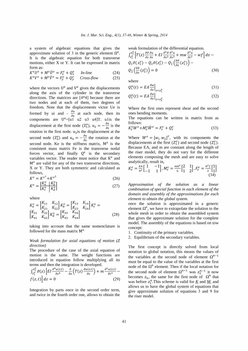
Fig. 3 provides an answer on how the internal

pressure and especially the perturbation component

affects the internal loading along the riser. The curves

in Fig. 3 show snapshots of the axial force F due to

the internal pressure for one excitation period after a

steady. State response has been attained. The

maximum of F occurs adequately far from the lower

end and the node of the maximum static moment.

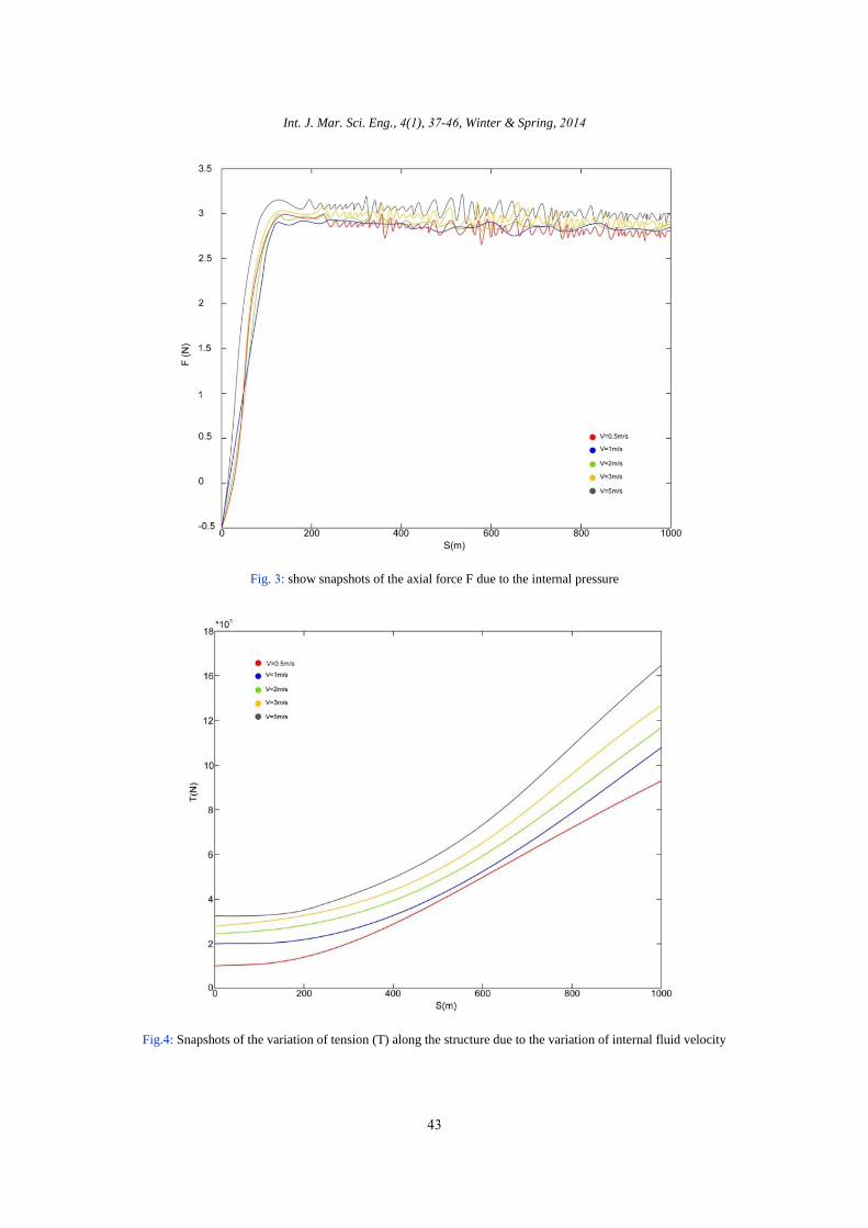
The effect of the flow inside the pipe can be

accurately represented by the simplified flow model.

To support this statement calculation, have been

performed with the contribution of the perturbation

component of the velocity field 𝜙 and the associated

results are depict in Fig. 4 These figures show

respectively the variation of tension T, for different

quantities of internal flow velocities, the in-line

bending moment and the out-of-plane bending

moment.

Fig. 5 and 6 show the response of the structure for

limited time domain under the velocity hydrodynamic

forces. In Fig. 5 the curves show the amount of

deflections.

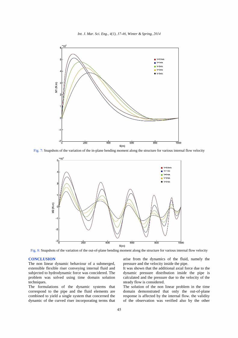
And finally Fig. 7 and 8 shows the variation of the in-

plane and out-of-plane bending moment along the

structure for various internal flow velocities. In fact

this curves are the results for solutions of differential

Equations.

Fig. 2: The response of the flexible riser under the static equilibrium

Int. J. Mar. Sci. Eng., 4(1), 37-46, Winter & Spring, 2014

43

Fig. 3: show snapshots of the axial force F due to the internal pressure

Fig.4: Snapshots of the variation of tension (T) along the structure due to the variation of internal fluid velocity

3D Finite element modeling for Dynamic Behavior Evaluation of Marin Risers

44

Fig. 5: Snapshots of the variations of the response the structure for the in-plane-direction

Fig. 6: Snapshots of the variations of the response the structure for the Out-of-plane-direction

Int. J. Mar. Sci. Eng., 4(1), 37-46, Winter & Spring, 2014

45

Fig. 7: Snapshots of the variation of the in-plane bending moment along the structure for various internal flow velocity

Fig. 8: Snapshots of the variation of the out-of-plane bending moment along the structure for various internal flow velocity

CONCLUSION

The non linear dynamic behaviour of a submerged,

extensible flexible riser conveying internal fluid and

subjected to hydrodynamic force was concidered. The

problem was solved using time domain solution

techniques.

The formulations of the dynamic systems that

correspond to the pipe and the fluid elements are

combined to yield a single system that concerned the

dynamic of the curved riser incorporating terms that

arise from the dynamics of the fluid, namely the

pressure and the velocity inside the pipe.

It was shown that the additional axial force due to the

dynamic pressure distribution inside the pipe is

calculated and the pressure due to the velocity of the

steady flow is considered.

The solution of the non linear problem in the time

domain demonstrated that only the out-of-plane

response is affected by the internal flow. the validity

of the observation was verified also by the other

M. Ghodsi Hassanabad and A. Fardad

46

numerical solution, that name is finite difference

method. It was shown that the Coriolis forces which

are incorporated into the dynamic system of the riser

due to the steady velocity term affect only the out-of-

plane motions reducing the magnitudes of the

associated dynamic components along the complete

length of the structure.

REFERENCES

Bar-Avi P., (2000). Dynamic response of risers

conveying fluid. Offshore Mech. Arctic. Eng. 122,

188- 193.

Chai Y.T., Varyani K.S., (2006). An absolute

coordinate formulation for three-dimensional

flexible pipe analysis. Ocean Eng 33, 23-58.

Chatjigeorgiou I.K., Damy G., Boulluec M., (2007).

Experimental investigation for the dynamic

behavior of a catenary riser under top imposed

excitations. In: Proceedings of the 7th

international

conference on cable dynamics, Paper No. 28.

Chatjigeorgiou I.K., Damy G., Le Boulluec M.,

(2007). Numerical and experimental investigation

for the dynamic behavior of a catenary riser under

top imposed excitations. In: Proceeding of the 7th

international conference on cable dynamics, Paper

No. 57.

Chucheepsakul S., Monprapussorn T., Huang T.,

(2003). Large strain formulation of extensible

flexible marine pipes transporting fluid. Fluids

struct. 17, 185 – 224.

Dupuis C., Rousselet J., (1992). The equations of

motion of curved pipes conveying fluid. Sound

Vibration 153, 473-489.

Francisco J., Huera H., (2006). Multi-mode Vortex-

Induced vibrations of a flexible circular cylinder.

PHD thesis, Department of aeronautics, university

of London.

Jain A.K., (1994). Review of flexible risers and

articulated storage systems. Ocean Engineering 21,

733-750.

Jain R., Jayaraman G.,(1990). On the steady laminar

flow in a curved pipe of varying elliptic cross-

section. Fluid Dynamics research 5, 351-362.

Kuiper G.L., Metrikine A.V., Efthymiou M., (2004).

Instability of a simplified model of a free hanging

riser conveying fluid. In: proceeding of the 23rd

international conference on offshore mechanics and

arctic engineering, Paper No.51.

LeCunff C., Biolley F., Damy G., (2005).

Experimental and numerical study of heave induced

lateral motion (HILM). In: Proceedings of the 24th

international conference on offshore mechanics and

arctic engineering, Paper No. 67.

Lin W., Qiao N., Yuying H., (2007). Dynamical

behaviors of a fluid-conveying curved pipe

subjected to motion constrains and harmonic

excitation. Sound Vibration 306, 955-967.

Misra A.K., Paidoussis M.P., Van K.S.,(1988). On

the dynamics of curved pipes transporting fluid.

Part II: Extensive theory. Fluids Struct. 2, 245-261.

Paidoussis M.P., (1998). Fluid-structure interactions:

Slender structures and axial flow. London

Academic Press 1, 24.

Paidoussis MP., (2001). Fluid-structure interactions:

Slender structures and axial flow. London

Academic press 2, 20

Paidoussis MP., (2005). Some unresolved issues in

fluid-structure interactions. Fluids struct 20, 871-

890

Patel HM, Seyed FB.,(1995). Review of flexible

risers modeling and analysis techniques.

Engineering Struct 17, 293 -304

Paulling J.R., Webster W.C., (1986). A consistent

large amplitude analysis of the coupled response of

a TLP and tendon system. In: Proceeding of the 5th

international conference on offshore mechanics and

arctic engineering, 126-133.

Petrakis M.A., Karahalios G.T., (1997).

Exponentially decaying flow in a gently curved

annular pipe. Int. J. of Non-Linear Mech. 32, 823-

835.

Qiao N., Lin W., Qin Q., (2006). Bifurcations and

chaotic motions of a curved pipe conveying fluid

with nonlinear constrains. Comput. Struct. 84, 708-

717.

Semler C., Li G.X., Paidoussis M.P., (1994). The

nonlinear equations of motion of pipes conveying

fluid. Sound Vibration 169,577-599.

Taniguchi A., Tanaka S., Yamashita K., Yoshizaw

M., (2007). Out-of-plane vibration of curved pipes

due to pulsating flow. In: EUROMECH colloquium

483, geometrically non-linear vibrations of

structures, 265- 268.

Wadham-Gagnon M, Paidoussis MP, Semler

C.,(2007). Dynamics of cantilevered pipes

conveying fluid. Part 1: Nonlinear equations of

three-dimensional motion. Fluid Struct 23, 545 -

567

Wu M.C., Lou J.Y.K., (1991). Effects of rigidity and

internal flow on marine riser dynamics. Appl.

Ocean Reaserch 13, 235 -244.

How to cite this article: (Harvard style)

Ghodsi Hassanabad, M *.; Fardad, A., (2014). 3D Finite element modeling for Dynamic Behavior Evaluation

of Marin Risers Due to VIV and Internal Flow. Int. J. Mar. Sci. Eng., 4 (1), 37-46.