3D Tomographic SAR Imaging: a status report

Lang Feng, Jan-Peter Muller

Imaging Group, Mullard Space Science Laboratory

(MSSL), University College London, Department of Space

& Climate Physics, Holmbury St Mary, Surrey, RH5 6NT,

UK – lang.feng.14@ucl.ac.uk, j.muller@ucl.ac.uk

3D&4D TomoSAR workflow

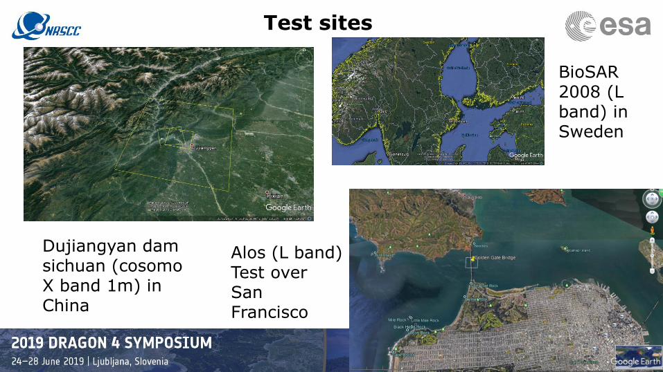
Test sites

BioSAR 2008 (L band) in Sweden

Dujiangyan dam sichuan (cosomoX band 1m) in China

Alos (L band) Test over San Francisco

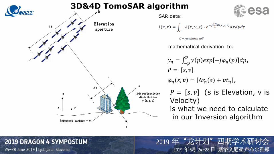
𝑦𝑛 = 𝑝−𝑝𝛾 𝑝 𝑒𝑥𝑝 −𝑗𝜑𝑛 𝑝 𝑑𝑝,

𝑃 = 𝑠, 𝑣

𝜑𝑛 𝑠, 𝑣 = ∆𝑟𝑛 𝑠 + 𝑣𝑡𝑛 ,

b

Elevation aperture

3-D reflectivity distributionγ(x,r,s)

Reference surface = 0

z

x y

Δb

Δs

γ

s

𝑃 = 𝑠, 𝑣 (s is Elevation, v isVelocity) is what we need to calculatein our Inversion algorithm

3D&4D TomoSAR algorithmSAR data:

mathematical derivation to:

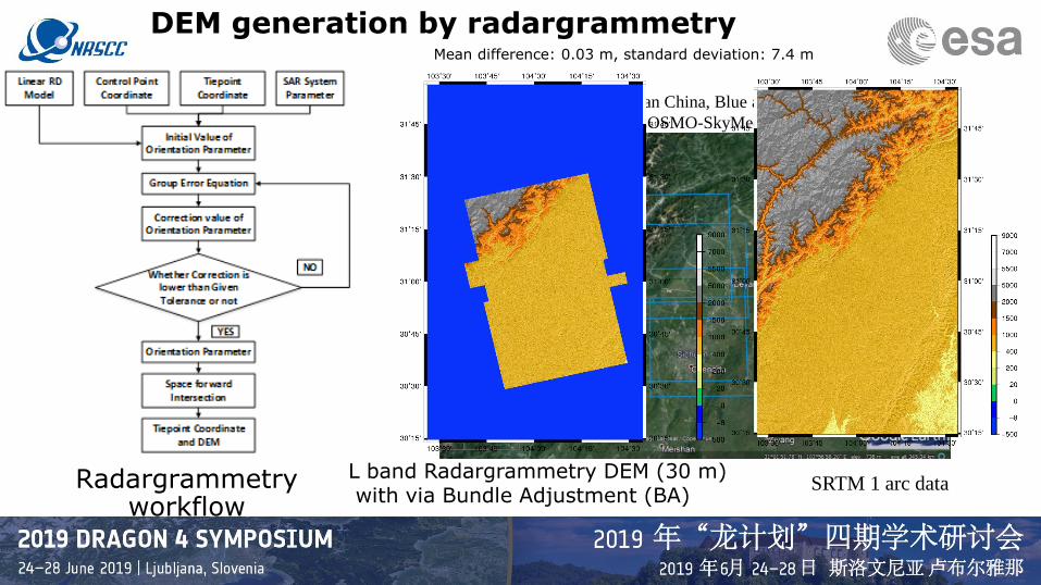
DEM generation by radargrammetry

L band Radargrammetry DEM (30 m)with via Bundle Adjustment (BA)

Radargrammetry workflow

SRTM 1 arc data

The test site in Sichuan China, Blue area is ALOS/PALSAR

data stacks, yellow area is COSMO-SkyMed Spotlight data stacks

Mean difference: 0.03 m, standard deviation: 7.4 m

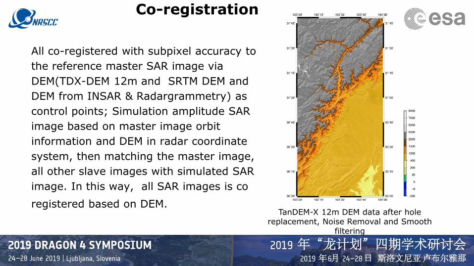
Co-registration

All co-registered with subpixel accuracy to

the reference master SAR image via

DEM(TDX-DEM 12m and SRTM DEM and

DEM from INSAR & Radargrammetry) as

control points; Simulation amplitude SAR

image based on master image orbit

information and DEM in radar coordinate

system, then matching the master image,

all other slave images with simulated SAR

image. In this way, all SAR images is co

registered based on DEM.TanDEM-X 12m DEM data after hole

replacement, Noise Removal and Smooth filtering

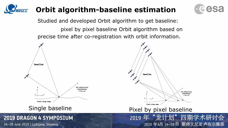
Orbit algorithm-baseline estimation

Studied and developed Orbit algorithm to get baseline:

pixel by pixel baseline Orbit algorithm based on

precise time after co-registration with orbit information.

Single baseline Pixel by pixel baseline

baseline

3-D reflectivity distributionγ(x,r,s)

Pixels along range

z

x y

s

baseline

3-D reflectivity distributionγ(x,r,s)

Pixels along range

z

x y

s

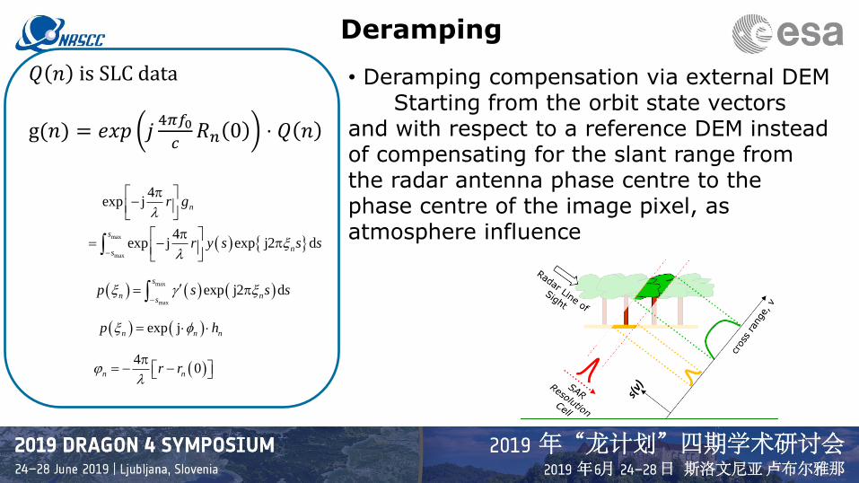
Deramping

4exp j nr g

−

( ) max

max

4exp j exp j2 d

s

ns

r y s s s−

= −

( ) ( ) ( )max

max

exp j2 ds

n ns

p s s s −

=

( ) ( )exp jn n np h =

( )4

0n nr r

= − −

• Deramping compensation via external DEMStarting from the orbit state vectors

and with respect to a reference DEM instead of compensating for the slant range from the radar antenna phase centre to the phase centre of the image pixel, as atmosphere influence

𝑄 𝑛 is SLC data

g(𝑛) = 𝑒𝑥𝑝 𝑗4𝜋𝑓0

𝑐𝑅𝑛 0 ⋅ 𝑄 𝑛

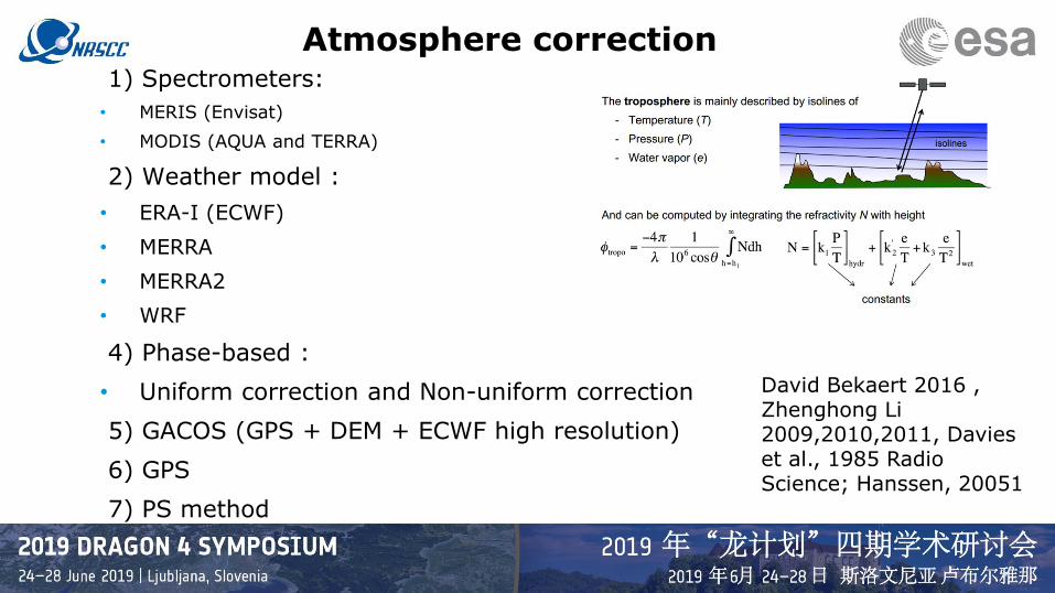
Atmosphere correction 1) Spectrometers:

• MERIS (Envisat)

• MODIS (AQUA and TERRA)

2) Weather model :

• ERA-I (ECWF)

• MERRA

• MERRA2

• WRF

4) Phase-based :

• Uniform correction and Non-uniform correction

5) GACOS (GPS + DEM + ECWF high resolution)

6) GPS

7) PS method

David Bekaert 2016 , Zhenghong Li 2009,2010,2011, Davies et al., 1985 Radio Science; Hanssen, 20051

TomoSAR- PS for atmosphere correction

Time and baseline plot

PS points in test area

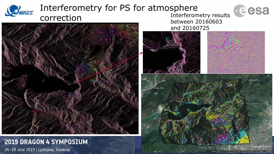
Interferometry for PS for atmosphere correction Interferometry results

between 20160603 and 20160725

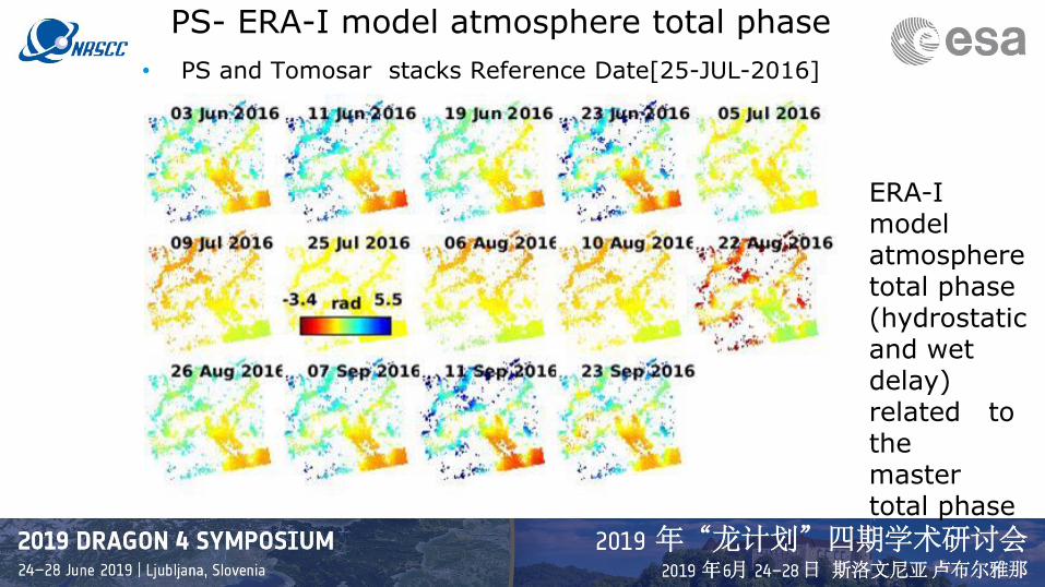
PS- ERA-I model atmosphere total phase

• PS and Tomosar stacks Reference Date[25-JUL-2016]

ERA-I model atmosphere total phase (hydrostatic and wet delay) related to the master total phase

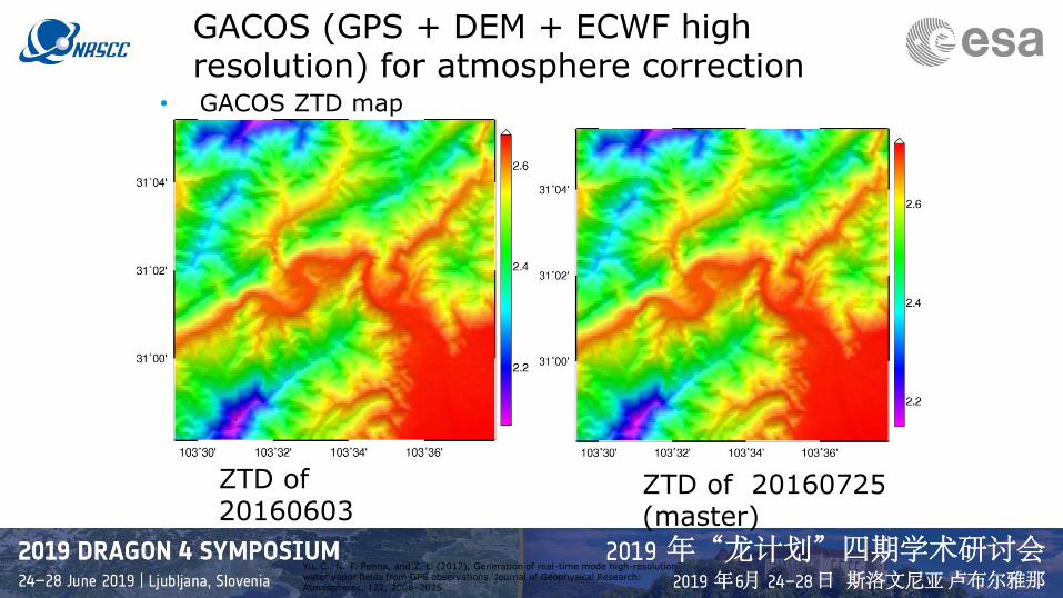
GACOS (GPS + DEM + ECWF high resolution) for atmosphere correction

• GACOS ZTD map

ZTD of 20160603

Yu, C., N. T. Penna, and Z. Li (2017), Generation of real-time mode high-resolution water vapor fields from GPS observations, Journal of Geophysical Research: Atmospheres, 122, 2008–2025.

ZTD of 20160725 (master)

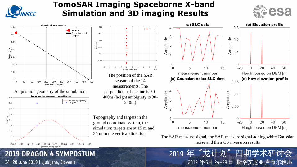
TomoSAR Imaging Spaceborne X-band Simulation and 3D imaging Results

Acquisition geometry of the simulation

Topography and targets in the

ground coordinate system, the

simulation targets are at 15 m and

35 m in the vertical directionThe SAR measure signal, the SAR measure signal adding white Gaussian

noise and their CS inversion results

The position of the SAR

sensors of the 14

measurements. The

perpendicular baseline is 50-

400m (height ambiguity is 30-

240m)

TomoSAR Results in Sweden

a) BioSAR 2008 in Sweden – ESA

b) SAR imaging in Sweden

c) Tomogram of red line in fig b via FFT

d) Coherence e) Orbit in x y plane

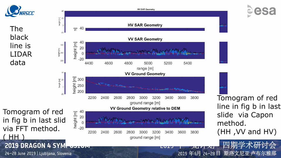
Tomogram of red line in fig b in last slide via FFT method. ( HH )

Tomogram of red line in fig b in last slide via Capon method. (HH ,VV and HV)

The black line is LIDAR data

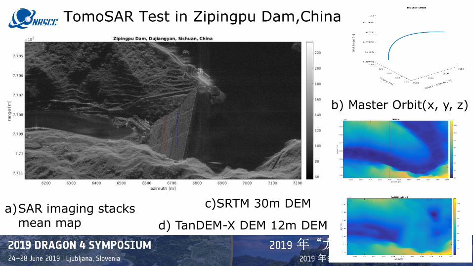
TomoSAR Test in Zipingpu Dam,China

a)SAR imaging stacks mean map d) TanDEM-X DEM 12m DEM

b) Master Orbit(x, y, z)

c)SRTM 30m DEM

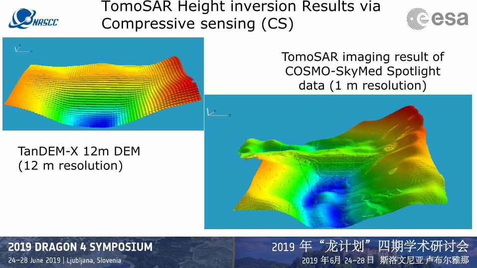
TanDEM-X 12m DEM (12 m resolution)

TomoSAR imaging result of COSMO-SkyMed Spotlight

data (1 m resolution)

TomoSAR Height inversion Results via Compressive sensing (CS)

TomoSAR Height and deformation Results via CS

(a) (b)

(c) (d)

1

D-TomoSAR velocity at

Zipingpu dam

3D display TomoSAR point cloud results at Zipingpu DAM ,China

3D display TomoSAR results

Field work for validation at Zipingpu dam

Difference map between X-band

TomoSAR imaging result and LIDAR data

Lidar point cloud of Zipingpu dam Chinese Gao fen Image

Basic Stats Area Min Max Mean(m) Stdev σ(m)

TomoSAR- LIDAR Dam and mountain trees 0 8.6 0.77 1.88

TomoSAR- LIDAR Dam 0 5.3 0.18 0.98

1

(b) 30 m SRTM data (c) 1m LIDAR DSM data

(d) final fused DEM data (5 m) (e) difference map between (c) and (d)

1

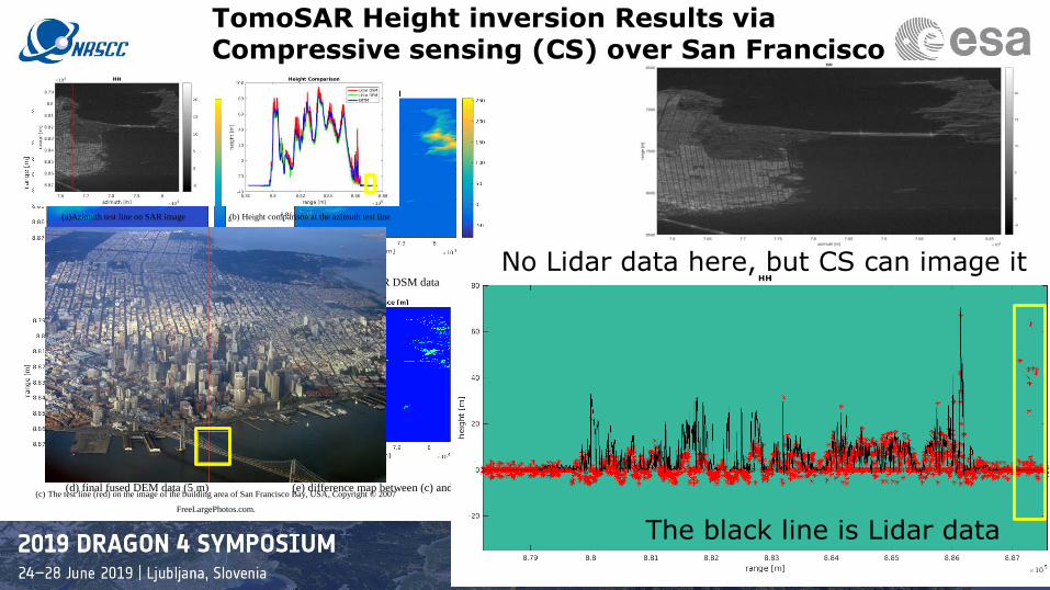
TomoSAR Height inversion Results via Compressive sensing (CS) over San Francisco

(a)Azimuth test line on SAR image (b) Height comparison at the azimuth test line

(c) The test line (red) on the image of the building area of San Francisco Bay, USA, Copyright © 2007

FreeLargePhotos.com.

1

No Lidar data here, but CS can image it

The black line is Lidar data

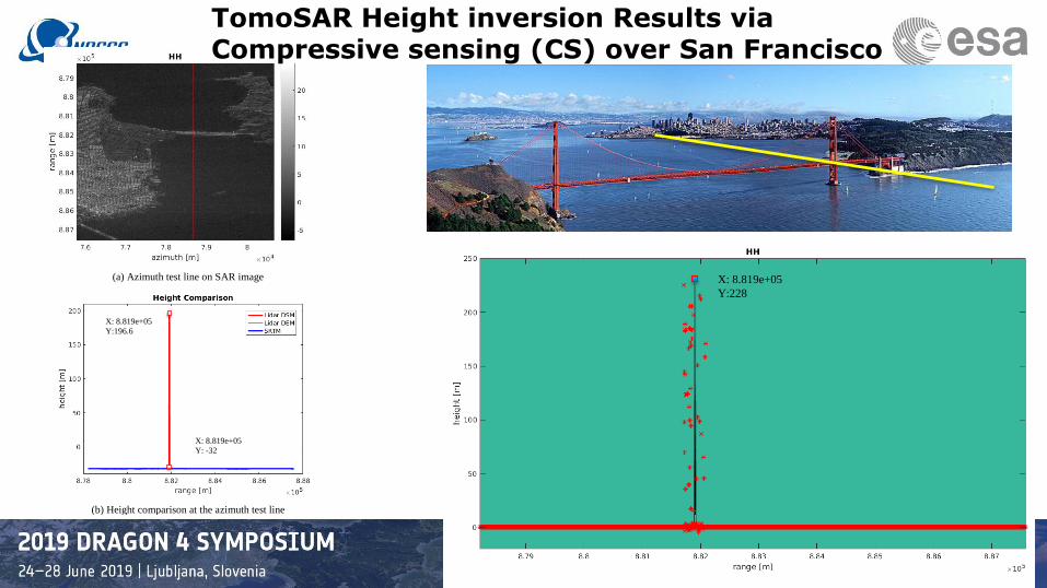
X: 8.819e+05

Y:228

(a) Azimuth test line on SAR image

(b) Height comparison at the azimuth test line

(c) The test line (yellow) on the image of the Golden Gate bridge of San Francisco Bay, USA ,

Copyright 2002 Strength in Perspective

1

X: 8.819e+05

Y:196.6

X: 8.819e+05

Y: -32

TomoSAR Height inversion Results via Compressive sensing (CS) over San Francisco

Conclusion• Tomographic data exhibit a more complex dependence of terrain

topography than traditional SAR data.

• Lidar forest height is not matched in Sar geometry, while it is well

matched in ground geometry relative to DEM.

• Orbital, tropospheric phase distortion and DEM correction are

indispensable in 3-D SAR imaging (SAR tomography) and 4-D SAR imaging

methods via Compressive sensing.

• The results demonstrate that L band data are fit for the structure

reconstruction of forests and manufacture facilities (bridge, building, and so

on), but the resolution is not very high. X band has little penetration

capability, which cannot be used for forest structure reconstruction.

However, it can be used for 3D TomoSAR imaging, the retrieval of the top

position of the canopy, the shape of the man-made structure (dam,

buildings and manufactured facilities) and the top of the 3D terrain, which

is best for high resolution DSM acquisition and target detection.

Acknowledgement

• Many thanks to CSC and UCL MAPS Dean prize through a PhD studentship at

UCL-MSSL.

• Many thanks to Space Catapult, Harwell space campus and Terri Freemantle,

in particular, for arranging the provision of CORSAIR011 data.

• Many thanks to Prof. jingfa Zhang, Dr. Qisong Jiao and Dr. Hongbo Jiang from

Institute of Crustal Dynamics, China Earthquake Administration for 2017 field work

and collaborations.

• Many thanks to Prof. Zhenhong Li for his valuable advice and providing GACOS

data.

• Many thanks to COMET for organizing INSAR TRAINING WORKSHOP 2017.

• Many thanks to Randolph Kirk (USGS), Elpitha Howington-Kraus (USGS) for

DEM code.

• Many thanks to Stefano Tebaldini (Politecnicodi Milano) , Laurent Ferro-Famil (

University of Rennes) for data and code and ESA for data and organizing the ESA

4th advanced course on radar polarimetry .