dvances in Optics and Photonics 2, 1–59 (2010) doi:10.1364/AOP.2.000001 2
Sfi
A
N
S
Tsntsmn
�
�
�
�
�
�
�
µ
�
�
�
�
�
A
A
c
f
G
G
g
h
k
L
Ln
n
N
NP
A
timulated Brillouin scattering in opticalbers
ndrey Kobyakov, Michael Sauer, and Dipak Chowdhury
otation
ymbols Used in the Text
he most frequently used symbols in this review are defined below, and corre-ponding units are given in square brackets. Dimensionless quantities are de-oted [ ]. The SI unit system is used throughout the review. Quantities related tohe optical power P can also be expressed in dBm �10 log10P �mW��. Italic sub-cripts denote running indices. Vector quantities are indicated in bold roman. Theagnitude of a vector is given by the corresponding italic letter, e.g., �B�=B. Acro-
yms used in the symbol table are defined in the acronym list below.
Symbol Unit Definition
�m−1� Loss coefficient of the optical fiber
R �m−1� Loss coefficient at the wavelength of Raman pump
�m−1 W−1� Peak SBS efficiency for fibers with a single dominant acoustic mode
m �m−1 W−1� Peak SBS efficiency corresponding to the mth acoustic mode
R �m−1 W−1� Raman efficiency
[ ] Dimensionless SBS efficiency
p [m] Pump wavelength
[ ] Fraction of the Stokes power relative to the pump power in the SBST definition
m �s−1� Brillouin frequency shift for the mth acoustic mode, �m=�p−�S��B for all m
p �s−1� Pump frequency, �p=2��p
S �s−1� Stokes frequency, �S=2��S
0 �kg/m3� Mean value of the material density
[W] Thermal noise power in the BGS bandwidth
m [ ] mth acoustic mode profile
[rad/s] Acoustic phonon frequency (single dominant acoustic mode), �=�p−�S
eff �m2� Optical effective area
mao �m2� Acousto-optic effective area corresponding to the mth acoustic mode
[m/s] Speed of light in vacuum
�r� [ ] Optical mode profile
��� [ ] Gain coefficient for the Stokes power in the noise initiated process
amp [ ] Gain coefficient in the Brillouin amplifier, PS�z=0�=GampPseed
m [m/W] Peak Brillouin gain for the mth acoustic mode
[J s] Planck’s constant
[J/K] Boltzmann’s constant
[m] Fiber length
��� [ ] Lorentzian profile of the Brillouin gain as a function of frequency
[ ] Effective refractive index of the fiber
sp [ ] Spontaneous emission factor in the SBS process
[ ] Number of photons emitted in the backward direction
A [ ] Numerical aperture of the fiber
p [W] Pump (forward propagating) power
dvances in Optics and Photonics 2, 1–59 (2010) doi:10.1364/AOP.2.000001 3
P
P
P
P
p
r
S
T
v
w
z
L
1
M1bpiRLUad
Bopap
A
0 [W] Input pump power, P0=Pp�z=0�
S [W] Stokes (backward propagating) power
seed [W] Input Stokes power into Brillouin amplifier, Pseed=PS�z=L�
th [W] SBST
12 [ ] Component of the electrostriction tensor
[m] Radial direction in the cylindrical coordinate system
[ ] Number of segments in a concatenated fiber link
[K] Absolute temperature
A [m/s] Acoustic velocity in the medium
m �s−1� FWHM of the BGS peak corresponding to the mth acoustic mode
[m] Coordinate along the fiber length
ist of Acronyms Used
BFABrillouin fiber amplifierBGSBrillouin gain spectrumDCFdispersion-compensating fiber
olecular scattering became a subject of intensive research in the 1920s and930s. Today, scattering from optical phonons (quantized states of the lattice vi-ration) is known as the Raman process, while interaction of light with acoustichonons is named after Léon Brillouin, who theoretically predicted light scatter-ng from thermally excited acoustic waves in 1922 [1]. Besides investigations byaman in India and Brillouin in France, molecular scattering was studied byandsberg and Mandelshtam in Russia, Smekal in Austria, and Wood in thenited States. Priorities of discoveries made at that time as well as the appropri-
teness of credits given are still being debated (see, e.g., [2,3], for a historicaliscussion).
rillouin scattering is one of the most prominent optical effects. In a spontane-us process, a photon from an incident light wave is transformed into a scatteredhoton and a phonon. The scattered wave is downshifted in frequency. It is calledStokes wave after George Stokes, who found the frequency downshift in the
rocess of luminescence in the 19th century. Typically, the scattering cross sec-
dvances in Optics and Photonics 2, 1–59 (2010) doi:10.1364/AOP.2.000001 4
tosttfwwie
Tpvltdqfipgt
S((ttTasS
A
ion of the Stokes light is quite low, but in optical fibers light can propagate tensf kilometers without significant attenuation. This makes (stimulated) Brillouincattering a noticeable and often undesirable effect in optical fibers. The scat-ered light has a certain angular distribution, but the fiber geometry selects onlywo preferred directions—forward and backward. As will be discussed below,orward Brillouin scattering in optical fibers is very weak. Therefore, the Stokesave propagates mainly in the direction opposite to the input, or pump, opticalave. At a particular level of the pump power, the process becomes stimulated,
.e., strongly dependent on the pump power. This is characterized by efficient en-rgy conversion from the input light to the backscattered wave.
he most prominent origin of stimulated Brillouin scattering (SBS) is a physicalhenomenon called electrostriction (see, e.g., [4]), which manifests itself in aariation of the medium’s density by action of light. The backscattered Stokesight interferes with the input pump light and generates an acoustic wave throughhe effect of electrostriction. Effectively, the propagating light creates a movingensity grating from which it scatters in the backward direction. Thus, the fre-uency downshift of the Stokes wave can also be explained by the Doppler ef-ect. The light scattering mechanism is schematically shown in Fig. 1. With thencreased intensity of the Stokes wave the interference pattern becomes moreronounced, and the acoustic wave increases in amplitude. The forward propa-ating acoustic wave acts as a Bragg grating, which scatters even more light inhe backward direction.
Figure 1
input opticalwave (pump)
spontaneouslybackscattered(Stokes) wave
input + reflectedinterference
spontaneousscattering
acoustic wavedue toelectrostriction
stimulatedscattering
stronger Stokeswave due toreflection frommoving grating
strongerinterference
pontaneous (top) and stimulated (bottom) Brillouin scattering. BackscatteredStokes) light (blue) from acoustic noise interferes with the input (pump) waveblack). The interference pattern is shown in red. The abscissa of the curves ishe coordinate along the medium length. The ordinate is the amplitude of the op-ical waves (black and blue curves) and the intensity of the interference (red).he amplitude of the acoustic wave is proportional to the optical intensity. Thecoustic wave generated as a result of electrostriction further stimulates back-cattering, which in turn enhances the interference between the pump and thetokes waves and reinforces the acoustic wave.
dvances in Optics and Photonics 2, 1–59 (2010) doi:10.1364/AOP.2.000001 5
Apsirp
Veidit[aBptbttSacScfit[is
RhsweeBia
Ocfootwborhs
A
lthough spontaneous Brillouin scattering was predicted in 1922, the stimulatedrocess, when the acoustic wave is created by the light beam itself, was only ob-erved in 1964 [5]. SBS is a nonlinear process, i.e., its efficiency depends on thenput power. The input signal power at which the Stokes wave power increasesapidly and may even be comparable with the input power is called the thresholdower or simply the SBS threshold (SBST).
arious fundamental and applied aspects of SBS were studied in the past. Forxample, the electrostrictive contribution to the intensity-dependent refractivendex was investigated both theoretically [6–10] and experimentally [11–14]. Aetailed model of a temporal response of the fiber’s refractive index is presentedn [10,15]. The effect of the refractive index profile on the Brillouin gain spec-rum (BGS) [16–21] and on the magnitude of the Brillouin gain coefficient22–28] was also the subject of numerous studies. The effect of Ge doping on thecoustic damping coefficient of silica fibers was studied in [29]. A very largerillouin gain coefficient was found in chalcogenide glasses [30,31]. Other im-ortant topics related to Brillouin scattering include polarization properties ofhe scattered light and acousto-optic polarization coupling [32–34], an interplayetween SBS and nonlinear four-wave mixing [35–38] or cross-phase modula-ion [39], as well as instabilities caused by the four-wave-mixing–SBS interac-ion [40,41], multicascaded SBS supported by Rayleigh backscattering [42],BS in distributed Er-doped fiber amplifiers (EDFAs) [43–45] and in Ramanmplifiers [46–50], the effect of spectrally broadened pump on scattering effi-iency [51,52], SBS in fiber Bragg gratings [53,54], and dynamic behavior ofBS [55–57], to mention only a few. The list of application areas where SBS be-omes relevant is even more extensive. One of the most prominent examples isber-optic telecommunications, where, for example, SBS may manifest itself
hrough the electrostrictive interaction between solitons in optical fibers58–64]. The impact of SBS on digital intensity-modulated signals is reviewedn [65,66], while SBS in amplitude-modulated cable television systems wastudied in [67–69].
esearch in SBS remains an actively developing area of nonlinear optics withundreds of papers published annually. It is certainly beyond the scope of aingle review to appropriately cover all the aspects of SBS. Therefore, in thisork we restrict ourselves to SBS in optical fibers and in particular focus on sev-ral of the most recent advances in the field. An extensive bibliography on thearlier work can be found in [70–72]. A detailed description of the physics ofrillouin scattering including the quantum-mechanical treatment can be found
n, e.g., [73,74], whereas topics related to fiber-optic telecommunication aspectsre covered in [75].
ur main goal in this review is twofold. First, we are going to discuss the spe-ifics of SBS in optical fibers. One key difference from SBS in crystals comesrom the extended spatial interaction between the pump and the Stokes waves inptical fibers. As a result, one needs to account for optical loss in noise initiationf SBS or in Brillouin amplification. Another difference from the bulk interac-ion is due to the guided nature of both optical and acoustic waves in the fiber. Itas recently observed that the guiding of longitudinal acoustic modes by the fi-er core is a very important effect. The dependence of the acoustic mode profilen the radial variation of the refractive index due to doping in the fiber core di-ectly affects the Brillouin gain magnitude. Fibers with different index profilesave different BGS and therefore different SBS thresholds [22,25,76]. Under-
tanding the acousto-optic interaction in a cylindrical guided wave geometry al-
dvances in Optics and Photonics 2, 1–59 (2010) doi:10.1364/AOP.2.000001 6
lstcdapiS
TscgoSmt
2S
Aeftottqc(eii
IonwS
T
fsaa
A
ows control of the Brillouin gain by index profile design. It should be empha-ized that guiding of both optical and acoustic modes is critical for an accurateheoretical description of the scattering process. For completeness, mathemati-al details of the derivation of the governing equations are presented in Appen-ix A. The second goal in our work is to give an overview of novel technologyreas where SBS plays an important role. These, for example, include high-ower fiber lasers, slow light, and optical delay lines for optical memory or SBSn Raman amplifiers and in radio-over-fiber transmission. We also briefly discussBS in multimode and photonic crystal fibers (PCFs)
he review is organized as follows. In Section 2 we outline the physics of thecattering process and introduce key concepts and parameters. We analyze theoupled evolutional equations derived in Appendix A to calculate the SBST andain of Brillouin fiber amplifiers (BFAs). Approaches to enhance the SBST ofptical fibers are discussed in Section 3, while several applications based onBS are reviewed in Section 4. Other fiber-optic issues such as SBS in multi-ode or microstructured fibers are considered in Section 5. Section 6 concludes
he paper.
. Key Physical Concepts of Inelastic Lightcattering
s was mentioned above, Brillouin scattering is caused by modulation of the di-lectric permittivity of the medium. The key distinction of Brillouin scatteringrom other types of molecular scattering is the acoustic type of the relevant lat-ice vibrations of the medium. For the acoustic mode, the direction of vibrationf the two neighboring atoms is the same, i.e., atoms oscillate with a small rela-ive phase shift. The type of dispersion relation of the acoustic mode (Fig. 2) de-ermines several key features of the scattered light such as a small relative fre-uency shift �10−5. The polarization induced by modulation of the refractive indexontains terms describing oscillations at the sum (anti-Stokes) and the differenceStokes) frequencies. The anti-Stokes emission is much weaker than the Stokesmission. In addition, it requires a seed wave at the sum frequency. Moreover, duringnteraction with the incident wave, the anti-Stokes wave is attenuated, i.e., its energys transferred to the incident pump wave [72,74].
n a quantum mechanical formulation, the process can be viewed as annihilationf the incident photon and creation of a scattered photon and an acoustic pho-on. The energy and the momentum of the interacting quanta must be conserved,hich results in a relation for the frequencies of the pump photon ��p�, thetokes photon ��S�, and the acoustic phonon ���,
�S = �p − � . �1�
he momentum conservation requires
�S = �p − B �2�
or the corresponding wave vectors. These relations can be shown in the disper-ion diagram (Fig. 2) on the coordinate plane �� ,�� [73]. Conservation laws (1)nd (2) then require a closed vector diagram for dispersion vectors �S, �p,
nd B.
dvances in Optics and Photonics 2, 1–59 (2010) doi:10.1364/AOP.2.000001 7
Tp2
natoB
wrEbqtmi
([dapzaostt
A
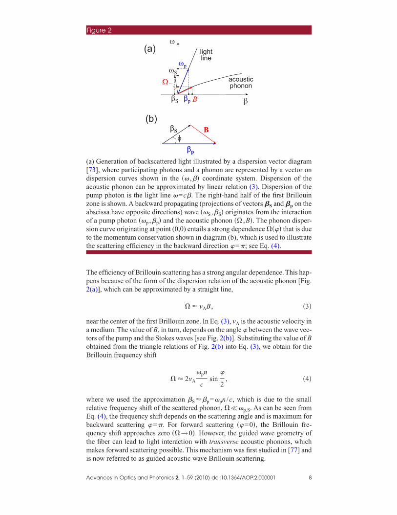
he efficiency of Brillouin scattering has a strong angular dependence. This hap-ens because of the form of the dispersion relation of the acoustic phonon [Fig.(a)], which can be approximated by a straight line,
� � vAB , �3�
ear the center of the first Brillouin zone. In Eq. (3), vA is the acoustic velocity inmedium. The value of B, in turn, depends on the angle between the wave vec-
ors of the pump and the Stokes waves [see Fig. 2(b)]. Substituting the value of Bbtained from the triangle relations of Fig. 2(b) into Eq. (3), we obtain for therillouin frequency shift
� � 2vA
�pn
csin
2, �4�
here we used the approximation �S��p=�pn /c, which is due to the smallelative frequency shift of the scattered phonon, ���p,S. As can be seen fromq. (4), the frequency shift depends on the scattering angle and is maximum forackward scattering =�. For forward scattering � =0�, the Brillouin fre-uency shift approaches zero ��→0�. However, the guided wave geometry ofhe fiber can lead to light interaction with transverse acoustic phonons, which
akes forward scattering possible. This mechanism was first studied in [77] and
Figure 2
�(a) light
line
�
acousticphonon
�p
B�p�S
�S�
(b)��S
�p
B�
a) Generation of backscattered light illustrated by a dispersion vector diagram73], where participating photons and a phonon are represented by a vector onispersion curves shown in the �� ,�� coordinate system. Dispersion of thecoustic phonon can be approximated by linear relation (3). Dispersion of theump photon is the light line �=c�. The right-hand half of the first Brillouinone is shown. A backward propagating (projections of vectors �S and �p on thebscissa have opposite directions) wave ��S ,�S� originates from the interactionf a pump photon ��p ,�p� and the acoustic phonon �� ,B�. The phonon disper-ion curve originating at point (0,0) entails a strong dependence �� � that is dueo the momentum conservation shown in diagram (b), which is used to illustratehe scattering efficiency in the backward direction =�; see Eq. (4).
s now referred to as guided acoustic wave Brillouin scattering.
dvances in Optics and Photonics 2, 1–59 (2010) doi:10.1364/AOP.2.000001 8
IeoSTSa
2P
Cwgaontwkdasda[
Btr
w
A
n Section 2.1 we present a detailed discussion of equations that describe thevolution of the guided pump and Stokes power caused by SBS in single-modeptical fibers. We then study the noise initiation of the backward propagatingtokes power in Section 2.2 and introduce the concept of SBST in Section 2.3.o initiate SBS, one can also launch a small amount of optical power at thetokes frequency from the opposite end of the fiber. Such a system will then acts an amplifier. BFAs are discussed in Section 2.4.
.1. Coupled SBS Equations for Evolution of Guided Opticalower
oupled SBS equations for the pump (forward propagating) and Stokes (back-ard propagating) light are extensively covered in the literature (see, e.g., mono-raphs [70,71,73] and textbooks [72,74]). However, in all mentioned referencesnd numerous research articles the derivation of evolutional equations is basedn the plane wave approach; i.e., guiding properties of participating waves areot accounted for. The plane wave approximation is also used in the fiber-opticextbooks [75,78,79] discussing SBS. It will be shown below why the planeave approximation provides good accuracy for step-index fibers. It is well-nown that acoustic waves can be guided in a solid cylinder [77,80–84] and in aouble-clad (fiberlike) structure [85–89]. Peral and Yariv [90] considered bothcoustic and optical guiding to describe the SBS process. However, their analy-is did not take into account the radial variation of mechanical properties of glassue to the refractive index variation in the core region. A more rigorous analysisccounting for the acoustic guiding by the doped core region was performed in22–25,28].
elow we analyze a set of coupled ordinary differential equations (ODEs) forhe spatial evolution of guided optical powers of the input pump Pp and the back-eflected Stokes PS wave (for a detailed derivation see Appendix A):
dPp
dz= − �mL���PpPS − �Pp, �5�
dPS
dz= − �mL���PpPS + �PS, �6�
Strictly speaking, in deriving evolutional SBS equathe plane wave approach is applicable only for amedium. In optical fibers, acoustic guiding effectsa crucial role and need to be accounted for to arately describe the scattering process.
tionsbulkplayccu-
here
dvances in Optics and Photonics 2, 1–59 (2010) doi:10.1364/AOP.2.000001 9
ifia
watf
U
ab3aautS
Swhsfio
A
�m =gm
Amao
�7�
s the peak SBS efficiency for the acoustic mode and � is the optical loss coef-cient of the fiber. The peak efficiency �m is inversely proportional to thecousto-optic effective area (see Appendix A):
Amao = � f 2�r�
m�r�f 2�r��2
m2 �r� , �8�
here f�r� and m�r� are radial profiles of the fundamental optical and the mthcoustic modes of the fiber, respectively.Angular brackets denote averaging over theransverse cross section of the fiber. Each acoustic mode is responsible for a spectraleature in the BGS (Fig. 3).
nlike the optical effective area, defined as [75,79]
Aeff =f 2�r�2
f 4�r��9�
nd conventionally used to characterize SBS in optical fibers, the quantity giveny Eq. (8) actually determines the total Brillouin gain. As we will see in Section, the acousto-optic effective area approximately equals Aeff for fiber profiles thatre close to step index. This explains why approximating Aao with Aeff gives goodgreement with experimental data when step-index, standard single-mode fibers aresed. However, for nonuniform fiber profiles, the parameter Am
ao rather than Aeff de-ermines the strength of the acousto-optic interaction and is responsible for differentBS thresholds in optical fibers with different index profiles. For example, counter-
Figure 3
noise-initiatedStokes wave
pump
w1
g1
frequency
power
�p
index profile
Pp
w2
�p-�1�p-�2
g2
rn
acoustic velocity
r
vA
PS
chematic representation of spectra of the pump (red) and the Stokes (blue)aves in an optical fiber with a non-step-index profile. In this example, the BGSas two peaks due to excitation of two dominant acoustic modes with frequencyhifts �1 and �2. Refractive index n�r� and acoustic velocity vA�r� profiles of theber are schematically shown in the top diagram to emphasize the guided naturef optical and acoustic waves in the fiber.
dvances in Optics and Photonics 2, 1–59 (2010) doi:10.1364/AOP.2.000001 10
ia
A
m
aocvotacraa[
T
wnwsvoa
TB
wl=qw
Fl
A
ntuitive results such as a higher SBS threshold for fibers with a smaller effectiverea were obtained [25,76].
related metric for the acousto-optic modal overlap was adopted in [25]. A di-
ensionless overlap integral Imao introduced there is the ratio of the optical and the
cousto-optic effective areas Imao=Aeff /Am
ao.This quantity (or, effectively, the acousto-ptic effective area) has been used in the full numerical modal analysis [27] to cal-ulate BGS of various fibers. Results obtained for F-doped step-index fibers showedery good agreement with measured data. The concept of the acousto-optic modalverlap was shown to be also applicable to Er–Yr doped fibers. Good agreement be-ween measured and calculated BGS was demonstrated in [91]. A 2D finite-elementnalysis [92,93] with the acousto-optic effective area used to calculate Brillouin gainorresponding to different acoustic modes demonstrated accurate prediction of BGSesonances for standard single-mode and PANDA (polarization-maintaining andbsorption-reducing) fibers. Similar analysis has been used to employ L01 and L03
coustic modes in w-shaped triple layer fibers for strain and temperature sensing94].
he numerator of Eq. (7) is the peak Brillouin gain of the mth acoustic mode gm,
gm =4�n8p12
2
c�p3�0�mwm
, �10�
here n is the effective refractive index of the fiber, p12 is the respective compo-ent of the electrostriction tensor, �m and wm are the frequency shift and the FWHMidth of the mth line in the BGS, respectively, �p is the pump wavelength, c is the
peed of light, and �0 is the mean value of the material density of the fiber. A typicalalue of �m for most germania-doped fibers is �11 GHz. For most fibers, it variesnly slightly (by �0.5 GHz) for different acoustic modes. Hence, without loss ofccuracy, one can use �m=�B for all acoustic modes in Eq. (10).
he nonlinear term in Eqs. (5) and (6) is multiplied by the spectral profile of therillouin gain L���, which has the Lorentzian shape
L��� =�wm/2�2
�� − �p + �m�2 + �wm/2�2, �11�
here �p=c /�p is the pump frequency. In the discussion of noise-initiated Bril-ouin scattering, we will assume the presence of a dominant acoustic mode (��1=g1 /A1
ao��m, m=2,3 ,4. . .), which is typical for single-mode fibers with auasi-rectangular index profile. This assumption will be relaxed in Section 3 whene will be discussing high-SBST fibers.
inally, several additional terms can be introduced in Eq. (7) to account for po-
The overlap integral between the optical and acomodes is responsible for different SBS thresholds otical fibers with different index profiles.
usticf op-
arization effects or the finite spectral line width wlas of the input signal,
dvances in Optics and Photonics 2, 1–59 (2010) doi:10.1364/AOP.2.000001 11
F2tpBgsg
2
TrtSa
TtSpstmmHcpaptS
Tcpge
wE
wc
A
�m =gm
AmaoK�1 +
wlas
wm . �12�
or a polarization-scrambled pump, the polarization factor K=3/2 differs frombecause of different Brillouin gains for spontaneous photons with a polariza-
ion identical with and orthogonal to the pump [34]. However, for high pumpowers the gain is much larger for copolarized Stokes and pump waves. At largerrillouin gains, SBS acts like an almost perfect polarization reflector with a de-ree of polarization close to 100% [32]. The term in parentheses in Eq. (12)hows that for a pump laser with a large spectral width wlas�wm the Brillouinain coefficient is reduced [18,66].
.2. Noise Initiation of SBS
o evaluate the critical input power, or SBST, one has to calculate the total back-eflected power at the fiber input, z=0. This is a difficult task because the scat-ering process starts spontaneously from noise; i.e., the boundary value of thetokes wave PS�L�, with L being the fiber length, is undetermined in ODEs (5)nd (6).
here are two standard models of noise initiation of SBS. In the framework ofhe localized, nonfluctuating source model, one assumes the presence of thetokes seed wave launched at the rear side of the lossless medium [71] or at theoint where loss exactly compensates for the Brillouin gain (the so-calledingle-photon approach discussed in [49,95]). According to a more rigorous dis-ributed, fluctuating source model, the backscattered wave originates from ther-
ally excited spontaneous phonons [49,96–101]. In [97,98,100], where thisodel was applied for short bulk media, the loss of the medium was ignored.owever, the contribution of loss is a very important effect in optical fibers be-
ause the pump–Stokes interaction occurs over long distances and both theump and the Stokes waves can be attenuated by orders of magnitude. For ex-mple, on propagation in a 50 km-long standard single-mode optical fiber the in-ut power is reduced to a level of 10% from its original value. In [99,101] the con-ribution of loss was accounted for to calculate the power spectral density of thetokes light.
he initiation of Brillouin scattering is accompanied by a low pump-to-Stokesonversion efficiency, and the undepleted pump approximation (UPA) can be ap-lied to solve the system of ODEs (5) and (6). Assuming the UPA, one can ne-lect the nonlinear term in Eq. (5) to find an approximate solution for the pumpvolution as Pp=P0e
−�z, which can be substituted into Eq. (6) to yield
dPS
dz= − �L���P0PSe−�z + �PS, �13�
here � is the gain parameter corresponding to the dominant acoustic mode.quation (13) can be rewritten for the photon occupation number as [95]
dN
dz= − �L���e−�zP0�N + nsp� + �N , �14�
here nsp=1+ �eh�B/kT−1�−1�kT / �h�B� and k and h are Boltzmann’s and Planck’s
onstants, respectively; T is the fiber temperature.
dvances in Optics and Photonics 2, 1–59 (2010) doi:10.1364/AOP.2.000001 12
Ssp
w
cTts
Tlcag
w
a
isfia
F
F
F
i
A
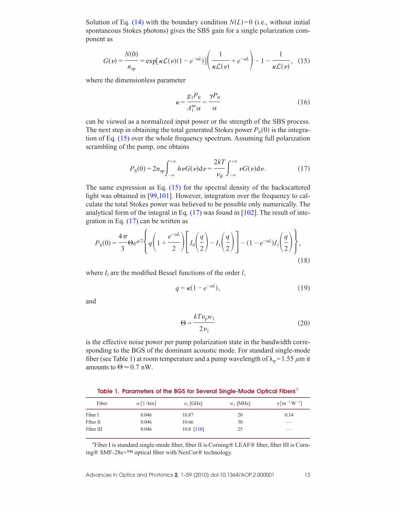
olution of Eq. (14) with the boundary condition N�L�=0 (i.e., without initialpontaneous Stokes photons) gives the SBS gain for a single polarization com-onent as
G��� =N�0�
nsp
= exp��L����1 − e−�L��� 1
�L���+ e−�L − 1 −
1
�L���, �15�
here the dimensionless parameter
� =g1P0
A1ao�
=�P0
��16�
an be viewed as a normalized input power or the strength of the SBS process.he next step in obtaining the total generated Stokes power PS�0� is the integra-
ion of Eq. (15) over the whole frequency spectrum. Assuming full polarizationcrambling of the pump, one obtains
PS�0� = 2nsp�−�
+�
h�G���d� =2kT
�B�
−�
+�
�G���d� . �17�
he same expression as Eq. (15) for the spectral density of the backscatteredight was obtained in [99,101]. However, integration over the frequency to cal-ulate the total Stokes power was believed to be possible only numerically. Thenalytical form of the integral in Eq. (17) was found in [102]. The result of inte-ration in Eq. (17) can be written as
PS�0� =4�
3eq/2�q�1 +
e−�L
2 �I0�q
2 − I1�q
2 � − �1 − e−�L�I1�q
2 � ,
�18�
here Il are the modified Bessel functions of the order l,
q = ��1 − e−�L� , �19�
nd
=kT�pw1
2�1
�20�
s the effective noise power per pump polarization state in the bandwidth corre-ponding to the BGS of the dominant acoustic mode. For standard single-modeber (see Table 1) at room temperature and a pump wavelength of �p=1.55 µm itmounts to �0.7 nW.
Table 1. Parameters of the BGS for Several Single-Mode Optical Fibersa
Fiber � �1/km� �1 [GHz] w1 [MHz] � �m−1 W−1�
iber I 0.046 10.87 20 0.14
iber II 0.046 10.66 30 —
iber III 0.046 10.8 [110] 25 —
aFiber I is standard single-mode fiber, fiber II is Corning® LEAF® fiber, fiber III is Corn-ng® SMF-28e+™ optical fiber with NexCor® technology.
dvances in Optics and Photonics 2, 1–59 (2010) doi:10.1364/AOP.2.000001 13
2
2
AmponµtpFv
wpa
2
Th(
w
i
Ddco
A
.3. SBS Threshold
.3a. Definitions
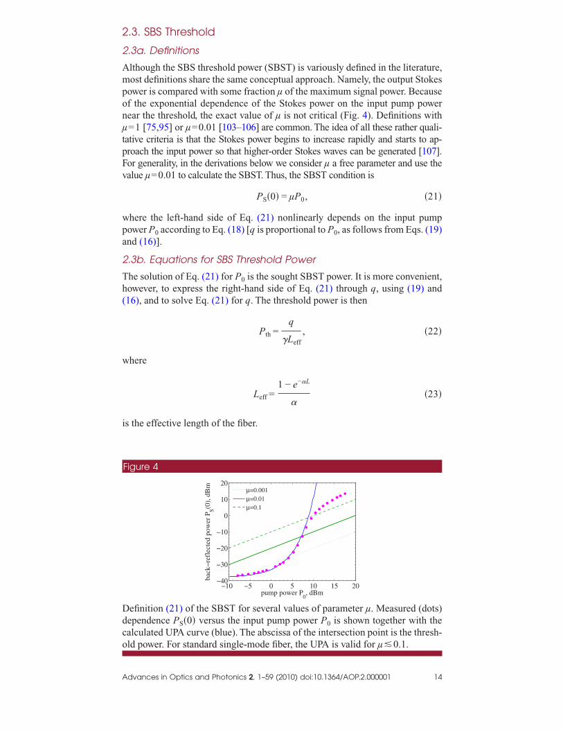
lthough the SBS threshold power (SBST) is variously defined in the literature,ost definitions share the same conceptual approach. Namely, the output Stokes
ower is compared with some fraction µ of the maximum signal power. Becausef the exponential dependence of the Stokes power on the input pump powerear the threshold, the exact value of µ is not critical (Fig. 4). Definitions with=1 [75,95] or µ=0.01 [103–106] are common. The idea of all these rather quali-
ative criteria is that the Stokes power begins to increase rapidly and starts to ap-roach the input power so that higher-order Stokes waves can be generated [107].or generality, in the derivations below we consider µ a free parameter and use thealue µ=0.01 to calculate the SBST. Thus, the SBST condition is
PS�0� = µP0, �21�
here the left-hand side of Eq. (21) nonlinearly depends on the input pumpower P0 according to Eq. (18) [q is proportional to P0, as follows from Eqs. (19)nd (16)].
.3b. Equations for SBS Threshold Power
he solution of Eq. (21) for P0 is the sought SBST power. It is more convenient,owever, to express the right-hand side of Eq. (21) through q, using (19) and16), and to solve Eq. (21) for q. The threshold power is then
Pth =q
�Leff
, �22�
here
Leff =1 − e−�L
��23�
s the effective length of the fiber.
Figure 4
−10 −5 0 5 10 15 20−40
−30
−20
−10
0
10
20
pump power P0, dBm
back
−re
flec
ted
pow
erP S(0
),dB
m µ=0.001µ=0.01µ=0.1
efinition (21) of the SBST for several values of parameter µ. Measured (dots)ependence PS�0� versus the input pump power P0 is shown together with thealculated UPA curve (blue). The abscissa of the intersection point is the thresh-ld power. For standard single-mode fiber, the UPA is valid for µ�0.1.
dvances in Optics and Photonics 2, 1–59 (2010) doi:10.1364/AOP.2.000001 14
At
a
N[db
Fb
T
w
Nt
2
FpccsSciAtcoLw
A
good approximation for Eq. (18) can be obtained if asymptotic expansions ofhe modified Bessel functions [108]
I0�x� �ex
�2�x�1 +
1
8x , I1�x� �
ex
�2�x�1 −
3
8x �24�
re used. The threshold equations (21) and (18) reduce to
�−3/2e��1−e−�L�
�1 − e−�L �e−�L +1
2� = µ
�
2���. �25�
early the same equation is obtained if the steepest descent method (see, e.g.,109], pp. 477–484) is used to perform integration in Eq. (17) [49,102]. The onlyifference compared with Eq. (25) is the second term in the parentheses, whichecomes 1/�.
or not very long fibers (L�40 km, ��0.2 dB/km), the term 1/ �2�� in (25) cane neglected, and the equation can be rewritten as
q3/2e−q =2���
µ�e−�L�1 − e−�L� . �26�
he approximate analytical solution of Eq. (26) is (see Appendix B)
q � ��1 +
3
2ln �
� −3
2� , �27�
here
� = − ln�2���
µ�e−�L�1 − e−�L�� . �28�
ext, Eqs. (27) and (28) can be substituted into Eq. (22) to obtain the value ofhe SBST.
.3c. Threshold Dependence on Fiber Length
igure 5 shows the measured dependence of the Stokes power PS�0� on the inputower P0 for various fiber lengths. Expressions derived in the previous sectionan be used for studying the SBST dependence on the fiber length as well as foromparing the accuracy of different approximations. Results for standardingle-mode fiber are shown in Fig. 6(a), where the calculated and measuredBST power Pth is plotted as a function of the fiber length. Parameters used in cal-ulations are shown in Table 1. As can be seen from Fig. 6(a), all approximations,ncluding the analytical solution (27), work well up to a fiber length of L�40 km.fter that distance, the accuracy of the short-fiber approximation decreases because
he term e−�L in Eq. (25) becomes comparable with the term 1/ �2��, which was dis-arded in the short-fiber approximation (26). For higher fiber loss (for example, forperation at shorter wavelengths) the short-fiber approximation remains accurate for�20 km [Fig. 6(b)]. The asymptotic expansion of the modified Bessel functions
orks well for all fiber lengths and attenuation coefficients.The error of the approxi-
dvances in Optics and Photonics 2, 1–59 (2010) doi:10.1364/AOP.2.000001 15
Rvw
(aoffi=
A
Figure 5
6 8 10 12 14 16 18 20−40
−30
−20
−10
0
10
input power, dBm
refl
ecte
dpo
wer
,dB
m
25.3 km20 km15 km10 km5 km2 km
eflected Stokes power PS�0� measured as a function of the input power P0 forarious fiber lengths. The threshold power can be obtained from definition (21),hich is shown by a dashed line �µ=0.01�.
Figure 6
a) SBST Pth in standard single-mode fiber. Pth is calculated exactly from Eqs. (21)nd (18) as well as by using several approximations: the asymptotic approximationf Bessel functions I0,1, Eq. (25); the short-fiber approximation (26); and analyticalormulas (27) and (28). Measured values of SBST obtained from Fig. 5 are shown bylled circles. (b) Same parameters as in (a) but the fiber loss is increased to �0.5 dB/km.
dvances in Optics and Photonics 2, 1–59 (2010) doi:10.1364/AOP.2.000001 16
mfitl
2F
Tt
wwa1cwt
wN=
a
e�(s
2
Sw
Da
A
ation does not exceed 0.3 dB. The accuracy of analytical formula (27) is quanti-ed in Fig. 7 for both values of the loss coefficient considered in Fig. 6.As expected,
he accuracy of the analytical approximation decreases with the increased fiberength and/or fiber loss (i.e., the product �L).
.3d. Origin of the Numerical Factor 21 in the Common SBSTormula
o complete the discussion on calculation of the SBST power, we briefly reviewhe widely used approximation (see, e.g., [31,75,95,111–114])
Pth = 21Aeff�
gB
, �29�
here gB=g1 is the peak Brillouin gain for the dominant acoustic mode. First, asas already mentioned, the optical effective area Aeff should be replaced with the
cousto-optic effective area A1ao. Formula (29) was first derived by Smith [95] in
972. The assumed fiber loss there was 20 dB/km, and terms with e−�L in Eq. (15)ould be safely discarded. After use of the steepest descent method in (17), Eq. (25)as obtained with the term �e−�L+1/ �2��� replaced with 1/�. As a result, the
hreshold equation took the form
�5/2e−� =��gB
�Aeff
, �30�
here µ=1 was assumed and power in only a single polarization was considered.ext, with �p=1.06 µm, �1=16.6 GHz, w1=50 MHz, [95] one obtains 1.8 nW, and for �=5�10−5 cm−1, gB=3�10−9 cm/W, and Aeff=10−7 cm2,
lso taken from Smith’s paper, the right-hand side of Eq. (30), which we denote �,
quates to 19.1�10−7. Then from Eq. (B.4) �� ��1+ �5/2�ln � / ��−5/2�� gives�21.1, and from the definition of � [Eq. (16)] one obtains the equivalent of Eq.
29). We also note that several authors [50,103,104,106,115] suggested using amaller numerical factor such as 17 or 18 in Eq. (29).
.4. Brillouin Fiber Amplifiers
BS can be used for efficient narrowband amplification when the seed Stokes
Figure 7
0 20 40 60 80 1000
0.5
1
1.5
2
fiber length L, km
erro
rof
anal
ytic
alfo
rmul
a,dB
α=0.2 dB/kmα=0.5 dB/km
ifference in SBST (decibels) between the exact value calculated from Eqs. (21)nd (18) and the value obtained from analytical formulas (27) and (28).
ave is input from the rear (opposite to the pump) end of the fiber. BFAs have
dvances in Optics and Photonics 2, 1–59 (2010) doi:10.1364/AOP.2.000001 17
aosaaws[gp
U(=pektf
SS
o[[mtpbt
Aa[orUmhn
A
pplications in microwave photonics, radio-over-fiber technology, and fiber-ptic sensing. For example, BFAs can be used to achieve gain in signal conver-ion in microwave photonic systems [116,117] or in the realization of a shape-djustable narrowband optical filter [118,119]. The same principle can also bepplied to carrier depletion for increasing the modulation depth of the micro-ave signal [120]. Optical carrier filtering in radio-over-fiber systems was
hown to significantly increase the dynamic range [121] and decrease the loss122] of microwave fiber-optic links. In addition, BFAs proved to be useful foreneration of millimeter-wave signals [123,124]. Most recently, BFAs were ex-loited as tunable slow-light delay buffers [125].
nlike the case of spontaneous Brillouin scattering, the system of ODEs (5) and6) for BFAs has well-defined boundary conditions: Pp�0�=P0 and PS�L�Pseed. Such a mathematical problem is known as the two-point boundary valueroblem. For systems of nonlinear ODEs, it is typically addressed numerically (see,.g., [126]). The exact solution to the boundary value problem of Eqs. (5) and (6) isnown only for lossless media [72,75,127], which cannot be used for BFAs, whereypically wave interaction occurs over tens of kilometers and loss is a significant ef-ect.
everal attempts have been undertaken to find a general analytical solution toBS equations in a lossy medium [101,128]. A conserved quantity
ln�PpPS� −�
��Pp − PS� = const, �31�
f the system of ODEs (5) and (6) reduces the problem to a single equation128], which, however, can only be integrated numerically. In another approach101], it was proposed to reverse the sign of the loss term in one of the ODEs toake the approximate set of equations integrable. This results in a system of two
ranscendental equations to be solved numerically with no closed-form solutionossible. Interestingly, a quite straightforward solution to the coupled ODEs cane obtained for copropagating scattered waves when the sign of both terms onhe right-hand side of Eq. (6) is reverted [129].
s another simplification, the UPA can be used. However, the above-mentionedpplications typically require pump powers above the SBS threshold116,120,122,124] so that the pump becomes depleted and the UPA stronglyverestimates the Brillouin gain. A straightforward method to improve the accu-acy of the UPA is a perturbative calculation of a first-order correction to thePA solution for the Stokes wave. Such an approach works well for a fiber Ra-an amplifier [130], which is described by a similar set of ODEs. One can show,
owever, that for SBS the perturbative correction to the UPA contains an expo-ential integral function that quickly diverges with increasing pump power.
If the perturbation approach in Brillouin amplificais applied to loss rather than to the nonlinear terclosed-form analytical solution to the coupledequations can be obtained
tionm, aBFA
dvances in Optics and Photonics 2, 1–59 (2010) doi:10.1364/AOP.2.000001 18
Tp
wawL
Fntagg[bc
MmP
A
he closed-form approximate analytical expression for Brillouin gain in the de-leted pump regime is [131]
Gamp =P0
Pseed�1 −
� + ln���1 − �/u��
u e−�L, �32�
here u=�P0L, �=−ln��PseedL�, and the BFA gain is defined as the ratio of themplified and the launched Stokes power, Gamp=PS�0� /Pseed. It is assumed that theavelength of the seed Stokes wave corresponds to the peak BGS frequency, i.e.,�1 in Eqs. (5) and (6). For comparison, the BFA gain calculated from the UPA is
GampUPA = exp�− �L + u
1 − e−�L
�L� . �33�
igure 8 compares the BFA gain obtained analytically from Eqs. (32) and (33),umerically from integration of Eqs. (5) and (6), and experimentally by usinghe setup shown in Fig. 9. A very good agreement between predictions of thenalytical formula (32) and the measured gain can be seen in the high gain re-ime. The accuracy of Eq. (32) decreases with increased fiber length but remainsood for BFAs shorter than 20 km. This is a typical length for many applications116,118,120,123]. Figure 8 also shows that for the weak-pump regime, the UPA-ased estimation for the Brillouin gain, Eq. (33), can be used. However, above someritical power P�Pcr���+��2+4�� / �2�L� Eq. (32) should be used instead.
Figure 8
easured and calculated gain of a 10 km long BFA based on standard single-ode fiber. The power of the input Stokes wave is (a) Pseed=−33 dBm and (b)
seed=−18 dBm.
dvances in Optics and Photonics 2, 1–59 (2010) doi:10.1364/AOP.2.000001 19
WaF
Itorwtsad
3
Sqhtgs
3
Fptpedo
EPfis
A
ith the increased Stokes seed power, the amplifier’s gain begins to saturate earlier,nd the maximum gain decreases compared with the case with smaller Pseed [cf.igs. 8(a) and 8(b)].
n the experimental setup (Fig. 9), a tunable laser with �p=1549.5 nm was usedogether with an EDFA to generate up to 70 mW of pump power.The seed wave wasbtained by using a Mach–Zehnder modulator (MZM). A fiber Bragg grating in theeflecting regime was used to select a sideband of the MZM output. Powermetersere used to monitor the input pump power P0, the transmitted pump power Pp�L�,
he launched seed power Pseed, and the amplified Stokes power PS�0�. The electricalpectrum analyzer was used to determine the Brillouin frequency shift of the fibernd, correspondingly, the modulation frequency for the MZM (10.88 GHz for stan-ard single-mode fiber).
. Fibers with Enhanced SBS Threshold
ome fiber-optic applications such as those discussed in the previous section re-uire high Brillouin gain to amplify the Stokes signal. In the majority of cases,owever, SBS is an undesired effect, since it prevents launching maximum op-ical power into the fiber. In these cases, it is desirable to decrease the Brillouinain coefficient � or, equivalently, increase the SBS threshold of the fiber. In thisection, we review several approaches that result in enhanced SBST of the fiber.
.1. Index-Controlled Acoustic Guiding
rom Eqs. (7), (8), and (10) one can conclude that one of the strongest controlarameters is provided by the acousto-optic effective area, Eq. (8). Even thoughhe optical mode profile might change only slightly from one single-mode fiberrofile to another, acoustic modes and corresponding acousto-optic effective ar-as can vary significantly. The SBS threshold in turn will depend on the fiber in-ex profile. To calculate the acoustic mode profile for a given index profile n�r�
Figure 9
TunableLaser MZM
~
10.877 GHz
PM
PM
PMPM
fiber
FBG
ElectricalSpectrumAnalyzer
OA
OA
VOA
VOA
coupler
circulator1549.5 nm
xperimental setup for BFA measurements: MZM, Mach–Zehnder modulator;M, powermeter; VOA, variable optical attenuator; OA, optical amplifier; FBG,ber Bragg grating used to select the upper modulation sideband as a Stokeseed signal.
ne has to solve the system of equations (A.12) and (A.13) for the acoustic mode
dvances in Optics and Photonics 2, 1–59 (2010) doi:10.1364/AOP.2.000001 20
pc
wcs
Tagm
PtP
A
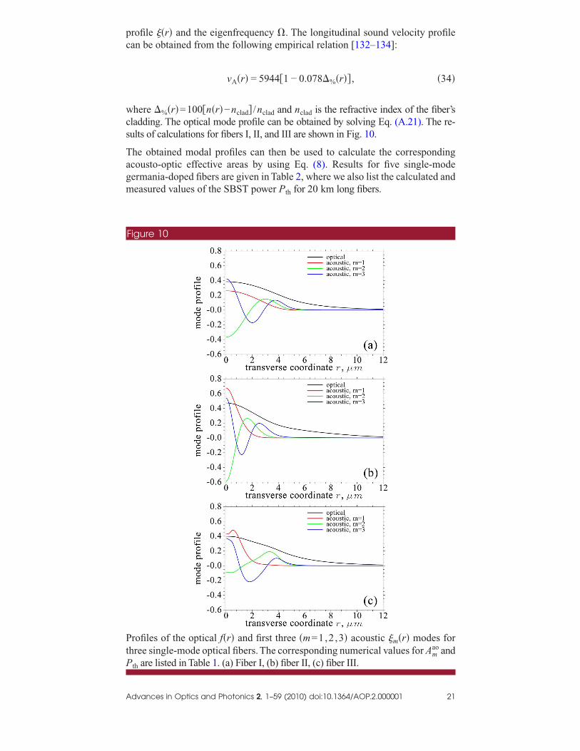
rofile �r� and the eigenfrequency �. The longitudinal sound velocity profilean be obtained from the following empirical relation [132–134]:
vA�r� = 5944�1 − 0.078�%�r�� , �34�
here �%�r�=100�n�r�−nclad� /nclad and nclad is the refractive index of the fiber’sladding. The optical mode profile can be obtained by solving Eq. (A.21). The re-ults of calculations for fibers I, II, and III are shown in Fig. 10.
he obtained modal profiles can then be used to calculate the correspondingcousto-optic effective areas by using Eq. (8). Results for five single-modeermania-doped fibers are given in Table 2, where we also list the calculated andeasured values of the SBST power Pth for 20 km long fibers.
Figure 10
rofiles of the optical f�r� and first three �m=1,2 ,3� acoustic m�r� modes forhree single-mode optical fibers. The corresponding numerical values for Am
ao and
th are listed in Table 1. (a) Fiber I, (b) fiber II, (c) fiber III.
dvances in Optics and Photonics 2, 1–59 (2010) doi:10.1364/AOP.2.000001 21
Cco
wm
Aoap(sS
w(mfi
We
MisficssI
F
F
F
F
F
b
A
alculation of the SBST has been performed by summing up reflected powerontributions from different acoustic modes, i.e., extending Eq. (17) to the casef multiple acoustic modes:
PS�0� = �m=1
M 2�T
�B�
−�
+�
�Gm���d� = µPS�0� , �35�
here Gm��� is the gain coefficient of Eq. (15) corresponding to the mth acousticode.
ccurate values of gm are difficult to obtain theoretically. We therefore make usef relative calculations of the SBS threshold. From the measured value of Pth forreference fiber I, which has only one dominant acoustic mode and thus a singleeak in the BGS, we obtain the value g1,ref from Eq. (26) [also using Eqs. (19) and16)]. Substitution of Eq. (15) into Eq. (35) with the subsequent integration by theteepest descent method results in the following transcendental equation for theBST:
e−�L
�1 − e−�L�m=1
M exp�rmkx�1 − e−�L��
�rmk
= x3/2µ�A11
ao
2��g1, �36�
here rmk=�mk /�1,ref��w11A11ao� / �wmkAmk
ao � and the index k denotes the fiber typesee Table 2), while the first index m denotes, as before, the number of the acousticode; x=Pthg1,ref / ��A11
ao�. The solution of Eq. (36) for x gives the SBST power forbers II–V from Table 2 as
Pthcalc = x
A11ao�
g1,ref
. �37�
e therefore assumed that the relative strength of the SBS interaction due toach acoustic mode is determined by the ratio rmk.
easured SBST powers were obtained from the corresponding reflected versusnput power curves (Fig. 11). The experimental setup is essentially the same ashown in Fig. 9, except no Stokes seed power is input to the fiber. All studiedbers have approximately the same attenuation coefficient �=0.2 dB/km. Asan be seen from Table 2, A1
ao for fiber I is smaller than that for fiber II. This is a con-equence of a weaker overlap between acoustic and optical modes. It leads to amaller Brillouin gain coefficient and consequently to a higher SBST power of fiber
Table 2. Calculated Acousto-optic and Optical Effective Areas ��m2� and Cal-culated and Measured SBST Pth [dBm]a
Fiber A1ao A2
ao A3ao Aeff Pth
calc Pthmeas
iber I 91.5 3928 4921 84.4 8.1 8.1
iber II 124.4 274.8 842 73.5 9.6 9.7
iber III 178.5 206.9 1539 85.4 11.2 11.5
iber IV 108.2 751.0 1641 88.0 8.9 9.2
iber V 112.0 161.8 2272 61.7 9.1 9.6
aFor single-mode optical fibers from Table 1 and two Ge-doped single-mode specialty fi-ers (fibers IV, V). All fibers are 20 km long.
I despite its smaller optical effective area compared with fiber I. Among the five
dvances in Optics and Photonics 2, 1–59 (2010) doi:10.1364/AOP.2.000001 22
caacE
Atas3c(tpia[
3
Adbdiniit
Toics
Mfi
A
onsidered single-mode fibers, fiber III has the largest acousto-optic effectiverea and thus the highest SBST. Even though its second acoustic mode 2�r� hascomparable overlap with the optical mode, the SBST power remains high be-
ause of the exponential dependence of Brillouin gain on the input power [seeq. (25)].
particular profile design can be used to increase the SBST. The increase in thehreshold value depends on the fiber type, since a change in the index profile alsoffects other important fiber parameters such as dispersion, loss, and bendingensitivity. For standard single-mode fiber (ITU G.652 compatible), an up todB threshold increase is possible [22].This value can be even higher for some spe-
ialty fibers such as highly nonlinear fibers [135]. Finally, we note that other dopantse.g., Al, F) used to modify the refractive index of pure silica may differently affecthe acoustic guiding. For example, F-doped silica has a smaller refractive index thanure silica and is therefore used as the cladding material. Since the acoustic velocityn F-doped silica is also reduced [19], fibers exploiting F doping have differentcoustic properties compared with Ge-doped fibers. A recent experimental study136] demonstrated that just using F doping does not increase the SBST of the fiber.
.2. Segmented Fibers
s was shown in Subsection 2.3c, the SBST of an optical fiber increases withecreased fiber length. This fact can be used to make fibers with increased SBSTy changing the Brillouin frequency shift �m along the fiber length [137–139]. Inoing so, one hinders the exponential growth of the backreflected power. Indeed,f BGS before and after some location z1 along the span length L �0�z1�L� doot overlap, the amount of Stokes power PS�z1� generated in the segment �z1 ,L�s not further amplified but is attenuated in the segment �0,z1� (see Fig. 12). SBSn nonuniform fibers has been studied experimentally [76,111,137–140] andheoretically [140,141].
he analysis of Subsection 2.2 can be extended to nonuniform fibers consistingf fiber pieces with different BGS. For a fiber span consisting of S segments (theth segment has length zi−zi−1) with nonoverlapping BGS, the total Stokes poweran be found from Eq. (17), where contributions from each fiber segment are
Figure 11
0 2 4 6 8 10 12 14 16 18 20−40
−30
−20
−10
0
10
20
input power, dBm
refl
ecte
dpo
wer
,dB
m
fiber Ifiber IIfiber III
easured reflected versus input power for the first three fibers in Table 2. Eachber length is 20 km. Definition (21) with µ=0.01 is shown as a dashed line.
ummed [140]:
dvances in Optics and Photonics 2, 1–59 (2010) doi:10.1364/AOP.2.000001 23
Iatmc
wsc
Taflfpswcfc
Sfaob
A
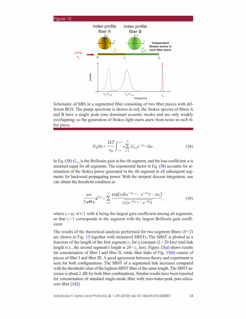
PS�0� =2kT
�B�
−�
+�
��i=1
S
G�,ie−�zi−1d� . �38�
n Eq. (38) G�,i is the Brillouin gain in the ith segment, and the loss coefficient � isssumed equal for all segments. The exponential factor in Eq. (38) accounts for at-enuation of the Stokes power generated in the ith segment in all subsequent seg-ents for backward propagating power. With the steepest descent integration, one
an obtain the threshold condition as
µ�
2���3/2 = �
i=1
S exp�ti��e−�zi−1 − e−�zi� − �zi�
�ti�e−�zi−1 − e−�zi�, �39�
here ti=�i / ��1 with � being the largest gain coefficient among all segments,o that ti=1 corresponds to the segment with the largest Brillouin gain coeffi-ient.
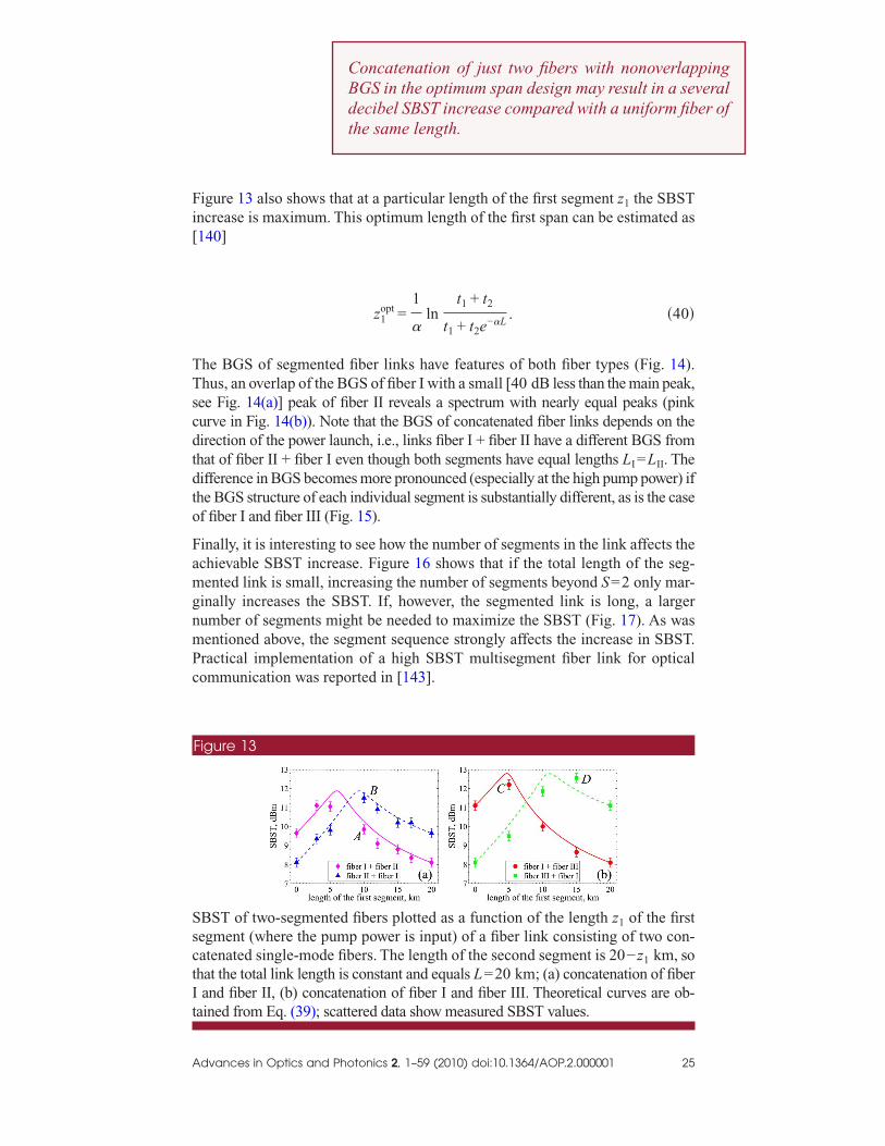
he results of the theoretical analysis performed for two-segment fibers �S=2�re shown in Fig. 13 together with measured SBSTs. The SBST is plotted as aunction of the length of the first segment z1 for a constant �L=20 km� total linkength (i.e., the second segment’s length is 20−z1 km). Figure 13(a) shows resultsor concatenation of fiber I and fiber II, while fiber links of Fig. 13(b) consist ofieces of fiber I and fiber III. A good agreement between theory and experiment iseen for both configurations. The SBST of a segmented link increases comparedith the threshold value of the highest-SBST fiber of the same length. The SBST in-
rease is about 2 dB for both fiber combinations. Similar results have been reportedor concatenation of standard single-mode fiber with zero-water-peak pure-silica-
Figure 12
independentStokes waves ineach fiber piece
pump
index profilefiber A
Pp
rn
r
PS,B
n
index profilefiber B
PS,A
0 z1 L
power
�p-�1,A�p-�1,B �pfrequency
chematic of SBS in a segmented fiber consisting of two fiber pieces with dif-erent BGS. The pump spectrum is shown in red; the Stokes spectra of fibers And B have a single peak (one dominant acoustic mode) and are only weaklyverlapping; so the generation of Stokes light starts anew from noise in each fi-er piece.
ore fiber [142].
dvances in Optics and Photonics 2, 1–59 (2010) doi:10.1364/AOP.2.000001 24
Fi[
TTscdtdto
FamgnmPc
SsctIt
A
igure 13 also shows that at a particular length of the first segment z1 the SBSTncrease is maximum. This optimum length of the first span can be estimated as140]
z1opt =
1
�ln
t1 + t2
t1 + t2e−�L
. �40�
he BGS of segmented fiber links have features of both fiber types (Fig. 14).hus, an overlap of the BGS of fiber I with a small [40 dB less than the main peak,ee Fig. 14(a)] peak of fiber II reveals a spectrum with nearly equal peaks (pinkurve in Fig. 14(b)). Note that the BGS of concatenated fiber links depends on theirection of the power launch, i.e., links fiber I + fiber II have a different BGS fromhat of fiber II + fiber I even though both segments have equal lengths LI=LII. Theifference in BGS becomes more pronounced (especially at the high pump power) ifhe BGS structure of each individual segment is substantially different, as is the casef fiber I and fiber III (Fig. 15).
inally, it is interesting to see how the number of segments in the link affects thechievable SBST increase. Figure 16 shows that if the total length of the seg-ented link is small, increasing the number of segments beyond S=2 only mar-
inally increases the SBST. If, however, the segmented link is long, a largerumber of segments might be needed to maximize the SBST (Fig. 17). As wasentioned above, the segment sequence strongly affects the increase in SBST.ractical implementation of a high SBST multisegment fiber link for opticalommunication was reported in [143].
Figure 13
BST of two-segmented fibers plotted as a function of the length z1 of the firstegment (where the pump power is input) of a fiber link consisting of two con-atenated single-mode fibers. The length of the second segment is 20−z1 km, sohat the total link length is constant and equals L=20 km; (a) concatenation of fiberand fiber II, (b) concatenation of fiber I and fiber III. Theoretical curves are ob-
ained from Eq. (39); scattered data show measured SBST values.
Concatenation of just two fibers with nonoverlapBGS in the optimum span design may result in a sevdecibel SBST increase compared with a uniform fibthe same length.
pingeral
er of
dvances in Optics and Photonics 2, 1–59 (2010) doi:10.1364/AOP.2.000001 25
3
Abc
(l=Ba9
Bifi
SsI
A
.3. Other Approaches to Suppress SBS
part from the discussed index control of the fiber core and using segmented fi-ers, a number of approaches can be employed to reduce the SBS efficiency. Oneommon method consists in broadening of the pump laser spectrum by using
Figure 14
a) BGS of fibers I and II measured with the electrical spectrum analyzer. Theength of each fiber is 20 km. The input power is Pp=8.1 dBm for fiber I and Pp
9.6 dBm for fiber II, corresponding to the SBST value for a given fiber length; (b)GS of concatenated spans of 10 km fiber I + 10 km fiber II (point A in Fig. 13(a))nd 10 km fiber II + 10 km fiber I (point B in Fig. 13(a)). The input power is.5 dBm for both configurations.
Figure 15
GS of concatenated spans of the total length of 20 km for several values of thenput power Pp: (a) 5 km fiber I +15 km fiber III (point C in Fig. 13(b)), (b) 15 kmber III + 5 km fiber I (point D in Fig. 13(b)).
Figure 16
BST of a 20 km long fiber link consisting of various numbers S of equal-lengthegments of alternating fiber I and fiber II: (a) fiber I + fiber II + fiber I + …; (b) fiberI + fiber I + fiber II + ….
dvances in Optics and Photonics 2, 1–59 (2010) doi:10.1364/AOP.2.000001 26
pcd
AsdwsdmoSpSla
AtdabSd
4
4
Tefpaa2w
IpI
A
hase modulation [144]. Then, according to Eq. (12) the Brillouin gain de-reases. This method is widely used in passive optical networks (PONs), e.g., forelivering a cable TV signal.
number of approaches are based on variation of fiber parameters such astrain, temperature, or core radius along the fiber length. For example, a strainistribution in the process of fiber cabling expanded the Brillouin gain band-idth from 50 to 400 MHz, which increased the SBST by �7 dB [145]. In another
tudy, a stair ramp strain distribution resulted in 8 dB SBST increase in a 580 mispersion-shifted fiber [146].The effective Brillouin gain was reduced by 3.5 dB byaking a core radius nonuniform along the fiber length [147]. In such an approach,
ne utilizes the dependence of the acoustic resonance frequency on the core radius.BST in a short, highly nonlinear fiber was increased threefold by applying a tem-erature distribution with a 140°C temperature gradient [148]. Another method ofBST enhancement consists in changing the dopant concentration along the fiber
ength [111,149]. The SBST increases nonlinearly with the dopant concentration �nd amounts, e.g., to 10 dB for �=0.15% when GeO2 is used as a dopant [149].
s a further design technique for SBS suppression, an acoustic antiguide struc-ure was proposed in [19]. This structure can be formed by doping the fiber clad-ing with F, which results in a decreased velocity of the acoustic wave in thisrea relative to the fiber core. However, it was found that this technique is limitedy cladding acoustic modes, which propagate along the core–cladding interface.everal other techniques are used to increase the SBST of fiber lasers. These areiscussed in Subsection 4.5.
. SBS in Fiber-Optic Applications
.1. Radio-over-Fiber Technology
ransmission of radio signals over optical fibers has long been recognized as anfficient method of RF signal distribution over longer distances (see, e.g., [150]or an overview). While such fiber-radio systems are often designed as point-to-oint links [151], there has been increasing interest in exploring access networkrchitectures where wireless services are distributed to subscriber’s homes fromcentral office (see Fig. 18 for a typical scenario). These services may compriseG/3G cellular, WiMAX (Worldwide Interoperability for Microwave Access),
Figure 17
ncrease in SBST versus total link length consisting of various numbers M ofairs of equal-length segments of alternating fiber I and fiber II; (a) fiber I + fiberI + fiber I + …; (b) fiber II + fiber I + fiber II +….
ireless local area network (WLAN), or other wireless signals. Such distribu-
dvances in Optics and Photonics 2, 1–59 (2010) doi:10.1364/AOP.2.000001 27
trm�lpqt[whwb
Tv(WtsluptEl
Fauc8
Atc
A
ion systems are typically based on PON architectures with high optical splittingatios close to the subscribers and up to 20 km signal distribution over single-ode fiber. In order to overcome high optical splitting ratios (typically 32� to 64) and maintain sufficient power levels at the receiving end, very high optical
aunch power levels are required. However, SBS plays an increasing role at higherower levels and can limit the performance of such networks and degrade the signaluality. Recently, there have been investigations of PON systems for radio signal dis-ribution that target applications like 3G cellular and WiMAX service distribution152–154], and SBS has been found to be a key limiting factor. A high-SBST fiberas shown to be beneficial for performance of hybrid fiber–coaxial and fiber-to-the-ome access networks [155]. Cost modeling also showed that deployment of fibersith a high SBST in fiber-to-the-home access networks can reduce material and la-or expenditures by more than 20% [156].
he performance of radio-over-fiber links can be characterized by the error-ector magnitude (EVM) [157], which is the quadrature amplitude modulationor QAM) constellation averaged SNR−2. According to the IEEE 802.11a/g
LAN standard, the EVM should be kept below 5.4% rms for highest data rateransmission.The dependence of EVM on the input power is shown in Fig. 19 for RFignal transmission over 20 km of fiber I and fiber III. At a very low input power theink performance is noise limited.An increase in the input power improves the EVMntil SBS starts to deteriorate the signal. With the increased amount of backreflectedower, the signal quality quickly degrades, and the EVM increases. A clear advan-age of the fiber with enhanced SBST can be seen by comparing the correspondingVM curves for fiber I and fiber III. The higher SBS threshold of fiber III allows for
ow EVM ��4%rms� for optical powers up to 17 dBm.
or experimental analysis of the RF signal quality of 802.11a/g WLAN packetsfter transmission over a PON system structure, a setup shown in Fig. 20 wassed. A distributed feedback laser signal was fed into an MZM via a polarizationontroller (PC). The modulator was biased at quadrature and modulated with an02.11 signal (orthogonal frequency-division multiplexing or OFDM, 64-
n example of an access network architecture. Optical signal is distributed fromhe central office through a feeder fiber and then transmitted further from the lo-al convergence point to network access points and premises.
dvances in Optics and Photonics 2, 1–59 (2010) doi:10.1364/AOP.2.000001 28
qnrvw1b
AbEb
4
RRcavartc
Mr
Eu
A
uadrature amplitude modulation) generated by a vector signal generator. Chan-els at both 2.4 and 5.8 GHz were used to represent 802.11g and 802.11a signals,espectively. The resulting optical signal was amplified with an EDFA and fed into aariable attenuator to control the fiber launch power. The maximum launch poweras about +17 dBm. After transmission, the signal was attenuated by an additional6 dB, representing the loss of an optical 32� splitter. The signal then was receivedy a standard photoreceiver, and the EVM was measured by a vector signal analyzer.
s was discussed in the previous section, an additional increase in the SBST cane achieved by using concatenated fiber spans. As can be seen from Fig. 21, theVM can be improved up to 1% rms and the signal power increased by �2 dBy using high-threshold concatenated spans [154].
.2. SBS in Raman-Pumped Fibers
aman amplification is widely used in telecommunication systems [158–160].aman amplifiers do not require an additional medium to amplify the signal, be-ause the fiber itself serves as an amplifying medium. Raman amplification hasdistributed nature. Therefore, the noise figure of the amplifier can be made
ery low to improve the optical SNR compared with EDFA-based systems. Thisdvantage in the noise performance becomes especially important for high-bit-ate transmission systems that have an elevated SNR requirement. Apart fromhe optical SNR improvement, Raman amplification enables a significant in-rease in the transmission bandwidth of the system [158].
easured EVM as a function of the optical input power for two values of the car-ier RF and two fiber types: fiber I and fiber III. The fiber length is 20 km.
Figure 20
fiber 20 km
DFB MZMPC
OA
VSG VOA 16 dB
Rx VSA
xperimental setup for RF transmission over a single-mode fiber. DFB, distrib-ted feedback laser; VSA, vector signal analyzer; VSG, vector signal generator.
dvances in Optics and Photonics 2, 1–59 (2010) doi:10.1364/AOP.2.000001 29
SBrwoaoattdTwasBs
Tppqtmmc
Foc
w
Mb2
A
timulated Raman scattering has many similarities to SBS. However, unlikerillouin scattering, the Raman effect is due to light interaction with optical
ather than acoustic phonons; i.e., molecular vibrations replace the acousticave in the scattering process. For typical crystals, the frequency of oscillationsf neighboring crystal planes as they move toward each other lies in the infrared,nd therefore that branch of dispersion is called “optical.” The dispersion curvef this optical mode does not originate from the point (�=0, �=0; see Fig. 2)nd thus has a nonzero frequency for �=0 (zero group velocity for the oscilla-ion mode). The dispersion curve of the optical phonon is flat near the center ofhe first Brillouin zone. Therefore, the frequency of scattered light only weaklyepends on the angle between wave vectors of input and scattered light waves.hat is why Raman scattering is almost equally efficient in forward and back-ard directions, and one can use both forward (copropagating with the signal)
nd backward (counterpropagating) schemes of Raman pumping. For Ramancattering, the frequency offset of the Stokes wave is much larger than in therillouin scattering and amounts to �13 THz in glass. Therefore, for a telecom
ignal at 1550 nm the pump wavelength lies in the range of 1400–1450 nm.
he Raman gain can be made quite high ��20 dB� so that the amplified signal’sower can approach the SBS threshold. This is especially true for forward Ramanumping.The bandwidth of a Raman amplifier is much larger than the Brillouin fre-uency shift. Therefore, the Raman pump will amplify not only the signal but alsohe Stokes wave, which then will experience gain from both SBS and stimulated Ra-an scattering so that a Raman pump will affect the SBST condition. As far as Ra-an pumping efficiency is concerned, several studies indicate that SBS, in turn,
auses saturation of the Raman gain [46–48,161].
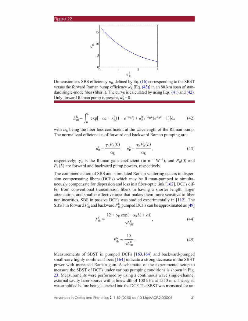
igure 22 shows how the SBS efficiency required in order to achieve the thresh-ld decreases in the presence of Raman pump. The dependence shown in Fig. 22an be approximated as [49]
�th �17
�LeffR
, �41�
R
Figure 21
2 4 6 8 10 12 14 16 181
1.5
2
2.5
3
3.5
4
input power, dBm
EV
M,%
rms
20 km fiber III15 km fiber III + 5 km fiber I
easured EVM versus optical input power for the concatenated span 15 km fi-er III +5 km fiber I for channel frequency of 5.8 GHz. Results for the uniform,0 km long fiber III are shown for comparison.
here the effective length due to Raman pumping, Leff, is given by
dvances in Optics and Photonics 2, 1–59 (2010) doi:10.1364/AOP.2.000001 30
wT
rP
TsnfanS
Mspm2ew
DvdO
A
LeffR = �
0
L
exp�− �z + �Rf �1 − e−�Rz� + �R
b e−�RL�e�Rz − 1��dz �42�
ith �R being the fiber loss coefficient at the wavelength of the Raman pump.he normalized efficiencies of forward and backward Raman pumping are
�Rf =
�RPR�0�
�R
, �Rb =
�RPR�L�
�R
, �43�
espectively; �R is the Raman gain coefficient (in m−1 W−1), and PR�0� and
R�L� are forward and backward pump powers, respectively.
he combined action of SBS and stimulated Raman scattering occurs in disper-ion compensating fibers (DCFs) which may be Raman-pumped to simulta-eously compensate for dispersion and loss in a fiber-optic link [162]. DCFs dif-er from conventional transmission fibers in having a shorter length, largerttenuation, and smaller effective area that makes them more sensitive to fiberonlinearities. SBS in passive DCFs was studied experimentally in [112]. TheBST in forward Pth
f and backward Pthb pumped DCFs can be approximated as [49]
Pthf �
12 + �R exp�− �RL� + �L
�LeffR
, �44�
Pthb �
15
�LeffR
. �45�
easurements of SBST in pumped DCFs [163,164] and backward-pumpedmall-core highly nonlinear fibers [164] indicate a strong decrease in the SBSTower with increased Raman gain. A schematic of the experimental setup toeasure the SBST of DCFs under various pumping conditions is shown in Fig.
3. Measurements were performed by using a continuous wave single-channelxternal cavity laser source with a linewidth of 100 kHz at 1550 nm. The signal
Figure 22
0 1 2 30
5
10
15
κRf
κth
imensionless SBS efficiency �th defined by Eq. (16) corresponding to the SBSTersus the forward Raman pump efficiency �R
f [Eq. (43)] in an 80 km span of stan-ard single-mode fiber (fiber I). The curve is calculated by using Eqs. (41) and (42).nly forward Raman pump is present, �R
b =0.
as amplified before being launched into the DCF. The SBST was measured for un-
dvances in Optics and Photonics 2, 1–59 (2010) doi:10.1364/AOP.2.000001 31
p1somtsbmr
Mbo(otl
4
Ai
Ed
Sc=
A
umped, forward, and backward-pumped DCFs with two Raman pumps centered at440 and 1460 nm. For theoretical calculations, this scheme was approximated by aingle pump at 1450 nm. Measurements were performed with Raman pump powersf 190, 280, and 380 mW, which correspond to on–off Raman gains of approxi-ately 10, 15, and 20 dB, respectively. The results of the measurements are shown,
ogether with results of calculations using Eqs. (44) and (45), in Fig. 24. As can beeen from the plot, the threshold power in forward-pumped fibers is less than that forackward pumping with the same Raman pump power. This implies that SBS isore detrimental in forward-pumped fibers than in backward-pumped fibers. Theo-
etical predictions for the SBST are in good agreement with measurements.
easurements of [164] imply that a decrease in SBST due to the presence of aackward Raman pump depends only on the net Raman gain (the fiber loss isffset) and does not depend on the fiber type. This trend can be seen from Eqs.45) and (42). Indeed, for backward pumping the difference in the SBST due ton–off Raman gain is �Pon−off �dB�=log10��1−e−�L�� /Leff
R , does not depend onhe Brillouin efficiency �, and for short fibers only weakly depends on the fibeross �.
.3. Slow Light and Optical Delay Lines
n interesting field for the application of SBS that resulted in intensive researchn recent years is the generation of slow light, where the group velocity of light
Figure 23
PCDFB OA
VOA
�������� DCFPM
circulator
forwardRaman pump
backwardRaman pump
1550 nm
xperimental setup for measurement of SBST in Raman-pumped DCFs. DFB,istributed feedback laser; PM, powermeter; PC, polarization controller.
Figure 24
0 100 200 300 400
−10
−5
0
5
Raman pump power, mW
SBST
,dB
m
forward pumpbackward pump
BST in a Raman-pumped DCF. Scattered data show measured values, dashedurves are calculated by using Eqs. (44) and (45). The DCF length is L10.5 km.
dvances in Optics and Photonics 2, 1–59 (2010) doi:10.1364/AOP.2.000001 32
pitcnlg
Frtt
TctHhaosreal
Sszo[tt1sq
Fclqtefcgnb
Aob
A
ropagation in a medium is significantly lower than its phase velocity [165]. Thiss achieved through increase in the group refractive index ng�1 by modifyinghe dispersion of the optical waveguide. The change in the group refractive indexan occur because of a narrow spectral resonance of a medium. Narrow reso-ances due to the SBS process are good candidates for changing the group ve-ocity of a pulse. The pulse delay �Tm due to the mth acoustic mode resonance isiven by [166,167]
�Tm =�mPpL
2�wm
. �46�
or the Stokes pulse, �m is positive (gain) and �Tm�0; i.e., the pulse is delayedelative to its propagation time in a nonresonant, passive medium. As was men-ioned above, �m�0 for the anti-Stokes pulse (i.e., the pulse is attenuated), andhe fast-light regime is realized.
he advantage of SBS versus other resonant techniques such as electromagneti-ally induced transparency or coherent population oscillation is the opportunityo control the pulse delay all-optically by varying the pump power [see Eq. (46)].owever, the Stokes pulse has to be i) centered precisely at the resonance and ii)ave a bandwidth smaller than wm. The use of SBS in optical fibers is especiallyttractive since it easily leads to the application of slow light in standard telecomperating windows, moderate pump powers, use of optical fibers as a transmis-ion medium, easy connection to standard telecom equipment, and operation atoom temperature [167–169]. Different types of fibers were considered for gen-ration of slow light. A comparative analysis of slica, bismuth oxide, tellurite,nd As2Se2 chalcogenide fibers can be found in [166]. More details on slow and fastight in optical fibers can be found in a recent review [167].
low light can be used for multiple applications in optical communications andignal processing, optical buffering and storage, jitter compensation, synchroni-ation of data, microwave photonics (e.g., phased array antennas), etc. The dem-nstrations of slow-light generation using SBS in optical fibers in 2005168,170] triggered an intensive wave of research in this field. The ability to ob-ain optical delays that can be controlled by the pump signal is very attractive forhe design of future optical systems. It was shown that 2 ns pulses (wavelength.55 µm) can be stored for up to 12 ns via SBS in a highly nonlinear fiber. Thetored pulses were then retrieved by a short intense read pulse having the same fre-uency as the pump pulse [171].
irst demonstrations of SBS-assisted slow light used a single pump wavelengthounterpropagating with the signal wavelength in an optical fiber. If both wave-engths are separated by the SBS acoustic wave frequency, i.e., Brillouin fre-uency shift (�11 GHz in standard optical fiber), a change in refractive index is ob-ained and the signal is slowed down. A side effect is the SBS gain that the signalxperiences, leading to an increase in the signal strength at the same time. Other ef-ects like potential signal distortion through increased dispersion need to be wellontrolled in order to avoid signal distortion beyond practical limits [172]. Since theoal of slow-light delay is to control the timing of optical signals, the data signaleeds to be detectable without major degradation, and error-free operation needs toe maintained.
n issue for practical applications is the very limited SBS gain bandwidth ofnly approximately 25 MHz in standard optical fibers. With such a small operating
andwidth, high-data-rate signals of 10 Gbit/ s and more cannot be effectively sup-
dvances in Optics and Photonics 2, 1–59 (2010) doi:10.1364/AOP.2.000001 33
p3t
Isswsbtb[
A2iocwetbt
Ftwetctic1�Rs
4
AdSdmtts
Amso
A
orted. Initial results showed that pulses of 100 ns could be slowed down by up to2 ns [170], and 63 ns pulses by up to 25 ns [168] without significant pulse distor-ion, demonstrating the potential of slow light by SBS in optical fibers.
n order to overcome the limited operating bandwidth of single-pump systems,everal investigations focused on the demonstration of multipump systems forlow-light generation. Since the total SBS power adds linearly for each pumpavelength, a superposition of the SBS gain spectra for multiple pump signals at
lightly different wavelengths will lead to a broadening of the resulting gainandwidth. Multiple techniques have been devised to design multipump genera-ors [173,174]. Comb lasers are an interesting way to generate multipeak pumpsecause of the ability to provide broad and uniform pump signal generation175].
significant breakthrough for broadband slow-light generation occurred in006 when a single pump laser was directly modulated with a noise signal, lead-ng to a very uniform SBS gain spectra of 325 MHz bandwidth [176]. Now, pulsesf only 2.7 ns duration could be delayed by more than a pulse width without signifi-ant distortion. This technique was later improved and used to generate a 12 GHzide SBS spectrum that allowed even 10 Gbit/ s signals to be delayed [177]. This
xperiment also explored the limits of single-pump SBS slow-light generation dueo the limited Brillouin frequency shift of �11 GHz. When the SBS gain becomesroader than the Brillouin frequency shift, a boundary for slow-light generation byhis technique is reached.
urther investigations led to the extension of the gain bandwidth by separatinghe pumps at twice the Brillouin gain shift. This led to an effective gain band-idth approaching 25 GHz [178]. Reaching bandwidths that allow 40 Gbits/ s and
ventually 100 Gbits/ s data transmission delay will be important for future sys-ems, and bandwidths of �50 GHz will be needed. Overall, there has been signifi-ant research to demonstrate the slow-light effect on real data transmission and proofhat error-free transmission with signal delay can be obtained [174,179]. While mostnvestigations focus on NRZ signals, differential phase-shift keying (DPSK) with itsonstant envelope behavior was also investigated [180]. A delay of 42 ps on a0.7 Gbit/ s NRZ-DPSK signal was demonstrated error-free with a power penalty10 dB. In comparing NRZ-DPSK and return-to-zero (RZ)-DPSK, it is shown thatZ-DPSK significantly outperforms NRZ-DPSK by 2 dB in power penalty at the
ame pump power.
.4. SBS-Based Fiber-Optic Sensors
n SBS-based distributed sensor relies on the temperature and strain depen-ence of the Brillouin frequency shift [181–187]. A schematic diagram of theBS-based sensing setup is shown in Fig. 25. A pulsed source is required in or-er to obtain positional information about stress or temperature variation byeans of time-delay analysis. The spatial resolution of a sensor is determined by
he pulse length and is usually limited to �1 m because of the finite responseime of the scattering process [188]. It is worth mentioning that the longitudinaltress is difficult to measure accurately with other techniques.
longitudinal strain of ���2�10−3 results in about a 100 MHz shift of the BGSaximum that is easily detectable [188]. However, a stable, narrowband tunable la-
er is required for reliable operation of the scheme. For example, a 50 m spatial res-−4
lution with a 10 strain sensitivity was achieved with a Nd:YAG ring laser (1 mW
dvances in Optics and Photonics 2, 1–59 (2010) doi:10.1364/AOP.2.000001 34
plwmcistm[
4
Allnfotpt
Asscesb
Hfimmf
Tgemah
St
A
ower, 5 kHz spectral line width) [189]. As for application areas, a distributed Bril-ouin sensor was used in civil engineering to identify and localize buckling [190] andall-thinning defects [191] in steel pipes. Another interesting example is healthonitoring of dams.A distributed temperature sensor has been used to monitor con-
rete setting temperatures of a large dam in Switzerland [183]. The fiber cable wasnstalled during the concrete pouring. A spatial resolution of 1 m and a temperatureensitivity of 1°C was demonstrated [183]. From the temperature variation duringhe setting chemical process one could determine the concrete density and identifyicrocracks. More details on Brillouin fiber sensors can be found in a recent paper
192].
.5. High-Power Fiber Lasers
detrimental effect of SBS in optical fibers can be observed in high-power fiberaser and amplifier designs. Because of the natural goal of generating high powerevels [193], the SBS threshold is easily reached in many designs, and tech-iques for SBS suppression are often required. While fiber lasers have uniqueeatures such as excellent beam quality, high efficiency, very high output powersf up to hundreds of watts, choice of lasing frequency (within limits), and ease ofhermal management, SBS is often the main limitation on achievable outputower for these devices. It therefore is of high interest to increase the SBShreshold in fiber laser designs [194].
widely used technique for SBS suppression is the modulation of the pump la-er source [68,144]. This leads to laser linewidth broadening and therefore to aignificant rise in SBS threshold by 10 dB or more. Multiple techniques can beonsidered: direct modulation of a semiconductor laser with a low-frequency signal,xternal phase modulation, or a combination of linewidth enhancing techniques. Be-ides pump linewidth broadening, the transmission–gain medium, i.e., the fiber, cane influenced to produce an increased SBS threshold.
igher-order modes can be used to essentially increase the effective area of theber, easily raising the SBS threshold significantly. In order to achieve single-ode designs, mode converters then need to be added [195]. The use of large-ode-area fibers also has been proposed [196] but is limited by operation in the
undamental fiber mode, which puts design restrictions on this approach.
he application of thermal gradients to the fiber was also extensively investi-ated. Either the absorption of the pump signal itself [197,198] or some form ofxternal gradient [199] was considered to increase the SBST. However, thermalanagement through either method is limited because too much heat is gener-
ted in the fiber core or too much external heat is applied. Nevertheless, several
Figure 25
pump, �p
pulsedlaser sensing
fiberSA
circulator Stokes, �p-�B
cw laser
chematic diagram of the SBS-based sensing setup. SA is the spectrum analyzerhat detects pump and Stokes signals.
undreds watts of power could be demonstrated by using such techniques.
dvances in Optics and Photonics 2, 1–59 (2010) doi:10.1364/AOP.2.000001 35
Aloiii(oat6ha
5
AmbSotflt
5
AaHnp[v5aSmlo
AmTw
w
A
nother technique includes the influence of the acousto-optic mode field over-ap in the fiber medium by design. It has been demonstrated that the Ge dopingf the core can be manipulated in such a way that the optical and acoustic fieldsn the fiber have significantly reduced overlap compared with standard step-ndex fibers and therefore raise the SBS threshold [22]. However, this techniques difficult to implement in large-mode-area fibers with low numerical apertureNA) where the dopant concentration is relatively small [194]. A technique tovercome this limitation was investigated in [200], where a combination of Gend Al doping was proposed. This way, the spatial separation between the acous-ic and optical fields was increased and the SBS threshold could be raised by
dB.A similar design led to an 11 dB SBS increase [201]. Using such designs, veryigh output powers of up to 500 W with narrow linewidth signals could bechieved [202].
. Other Fiber-Optic Issues
s was shown above, even if a fiber is single-mode with respect to opticalodes, it can be multimode with respect to acoustic modes, and it is the overlap
etween the fundamental optical and the acoustic modes that determines theBS efficiency. The situation becomes even more involved if either the numberf optical modes increases or the shape of the optical and acoustic modes dras-ically changes, for example, if modes become more tightly localized. Theormer situation takes place in large-core multimode fibers (MMFs), while theatter is typical for the small-core PCFs. Below, we briefly review SBS peculiari-ies in these fiber types.
.1. SBS in Multimode Fibers
rigorous treatment of multiple modes (both optical and acoustic) in a large-rea glass cylinder with a graded-index profile seems to be very complicated.owever, good agreement with measured data for the SBST is achieved if theominal core area of a MMF, �rc
2, where rc is the radius of the fiber core, is re-laced with some effective area �reff
2 with the effective mode radius reff�rc
203,204]. Then, the standard threshold equation (30) was used to obtain the SBSTalue for MMFs. For a multimode graded-index fiber with a core diameter of0 µm, cladding diameter of 125 µm, and length of 4.4 km, the effective mode di-meter was found to be 20.6 µm, which explained the experimentally determinedBST of 100 mW. Using the plane wave approach resulted in �4 times overesti-ation of the threshold power [203]. It was also found that the gain coefficient for
ower-order modes strongly exceeds (by a factor of �16) the gain of the higher-rder modes [205].
n analytical estimate for the SBST increase in MMFs compared with a single-ode fiber was derived in [206]. A step-index profile of the MMF was assumed.he ratio of the SBST power in a MMF to that in a single-mode fiber Pth can beritten as
PthMMF
Pth
=Y
arctan Y, �47�
here
dvances in Optics and Photonics 2, 1–59 (2010) doi:10.1364/AOP.2.000001 36
witt
Fv�irm
5
Mobcsapnfitvocvta
Ats(occbPPtls
A
Y =vA�ncore − nclad�
�pw, �48�
is the FWHM of the BGS, and ncore and nclad are the core and cladding refractivendices, respectively. It was assumed that the mode with the maximum gain induceshe SBS process. For small-numerical-aperture fibers, Eq. (48) can be expressedhrough the NA parameter as
Y =vANA2
2ncore�pw. �49�
or most commercial MMFs, the numerical aperture is NA�0.2. In this case, thealue of Pth
MMF/Pth estimated from Eq. (47) amounts to 1.8 for the pump wavelength
p=1 µm [206]. A further increase in the SBST accuracy in MMFs can be obtainedf one accounts for the inhomogeneous broadening of the Brillouin gain [207]. In aecent work [208], an approximation for the BGS shape was proposed based on nu-erical evaluation of the overlap between optical and acoustic modes.
.2. SBS in Microstructured Fibers
icrostructured fibers—also called holey fibers or PCFs—demonstrate numer-us novel effects of light propagation such as endlessly single-mode operation orandgap guiding [209]. Periodicity of the refractive index variation in the fiber’sross section and small core of a PCF strongly increase confinement of light andound and may drastically change the dispersion relation of both optical andcoustic modes. This changes the acoustic guiding properties of the fiber com-ared with standard single-mode fiber. As a result, a BGS may contain reso-ances corresponding to not only longitudinal (as in conventional single-modebers) acoustic modes but also to shear modes or coupled states between longi-
udinal and shear modes. For small-core PCFs (core diameter is less than theacuum wavelength), a multi-peaked BGS with Brillouin shifts �10 GHz wasbserved [210]. One can observe a relatively strong forward scattering Brillouin pro-ess, similar in nature to Raman scattering even though acoustic phonons are in-olved [211]. PCFs typically behave as acoustic antiguides because, unlike conven-ional fibers with Ge-doped cores, the holey cladding has a significantly lowercoustic index compared with the core.
mong other interesting features of Brillouin scattering in PCFs, one can men-ion both increased (up to �100 relative to fused silica [212] in a PCF based onulfide glass) and reduced [105] Brillouin gain, strong polarization dependence3 dB SBST difference between two polarizations) of the Brillouin gain [213,214],r reduced guided acoustic wave Brillouin scattering noise [215,216], which can fa-ilitate experiments operating at the quantum noise limit. It was found that with de-reasing core size, the SBST increases faster than in a conventional single-mode fi-er [213]. This is attributed to the diffraction of the acoustic wave out of the smallCF core and the acoustic antiguiding of PCFs. Acoustic resonances in nonlinearCFs were shown to be controllable coherently. Depending on the time delay be-
ween two pulses launched into the PCF, the acoustic resonance in the forward Bril-ouin spectrum could be either coherently reinforced or suppressed [217]. To ob-
erve the effect, the pulse delay should be well within the lifetime of the acoustic
dvances in Optics and Photonics 2, 1–59 (2010) doi:10.1364/AOP.2.000001 37
rlP
6
WltattvmBfoW
ASWMtm
w=gsesa
Tp
w=tfc
A
esonance ��11 ns�. Small-core PCFs also show promise in enhancing the slow-ight delay. For example, up to one-half pulse width delay was achieved in a 50 mCF by using a single pump [218].
. Conclusions
e have reviewed stimulated Brillouin scattering (SBS) in optical fibers. Bril-ouin gain of a fiber depends on the index profile through the overlap integral be-ween the acoustic mode profile and the squared optical mode profile. We havelso introduced the acousto-optic effective area, which is inversely proportionalo the Brillouin gain coefficient. Analytical results for the noise-initiated SBShreshold obtained from different approximations were analyzed. We also re-iewed several approaches to control Brillouin gain in the fiber. An attractiveethod is an index profile design that can be used to both suppress and enhancerillouin gain. We also discussed BFAs and distributed sensors. Several recently
eatured SBS-based or SBS-related applications were reviewed, such as radio-ver-fiber technology, slow light and optical delay lines, and high-power lasers.e have also discussed SBS in large-core multimode and PCFs.
ppendix A: Derivation of Evolutional Equations forignal and Stokes Wavese start our analysis with the material density equation (acoustic wave) andaxwell’s equations (optical waves) and present intermediate results to make
he derivation easy to follow. First, we look for a solution of the equation for theaterial density [70–72,90]
�2�
�t2− ��2
��
�t− vA
2 �r��2� = −�e
2�2E2, �A.1�
here � �kg/m3� is the material density fluctuation around its mean value �0, ��11/�0 �m2/s� is the damping factor, vA
2 �r�=Y�r� /��r� �m2/s2� is the squared lon-itudinal sound velocity that depends on the transverse radial coordinate r due toilica doping with GeO2, Y�r� [Pa] is theYoung’s modulus, �e=n4�0p12 [F/m] is thelectrostriction constant, n is the glass refraction index, �11 [Pa s] and p12 [dimen-ionless] are the respective components of the viscosity and electrostriction tensors,nd �0 is the vacuum permittivity.
he electric field E on the right-hand side of Eq. (A.1) is represented as a super-osition of forward- and backward-propagating electromagnetic waves:
here f�r� is the dimensionless fundamental optical mode profile; Aj�z , t�, j1,2, are the slowly varying envelopes of the optical field; uj are unit vectors in
he forward and backward direction of propagation; �j and �j are, respectively,requencies and propagation constants of optical waves; and c.c. denotes the
omplex conjugate. Then the right-hand side of Eq. (A.1) takes the form
dvances in Optics and Photonics 2, 1–59 (2010) doi:10.1364/AOP.2.000001 38
wis
AW
wfr
ws
�p
B(rjwp
A
�2E2 � −1
2f 2�r�A1�z,t�A2
*�z,t��s2ei��dt−�sz� + c.c., �A.3�
here �d��1−�2 and �s��1+�2�2�1neff /c�4�n /� with neff, �, and c be-ng the effective refractive index of the optical mode, input signal wavelength, andpeed of light, respectively.
.1. Stationary Solution for the Density Variatione look for the solution of Eq. (A.1) in the form
��z,t,r,�� =1
2�m=1
M
�m�z,t�m�r,��ei��t−qz� + c.c., �A.4�
here M is the number of acoustic modes of the optical fiber, � is the acousticrequency, and q is the corresponding wave vector of the density variation. Theespective derivatives of the material density are
��
�t=
1
2�m=1
M � ��m
�t+ i��m mei��t−qz�,
�2�
�t2=
1
2�m=1
M � �2�m
�t2+ 2i�
��m
�t− �2�m mei��t−qz�,
�2�
�z2=
1
2�m=1
M � �2�m
�z2− 2iq
��m
�z− q2�m mei��t−qz�,
here +c.c. terms are assumed on the right-hand side. With all this, the left-handide of Eq. (A.1) can be written as 1
2�m=1M ei��t−qz�S, where
S = m� �2�m
�t2+ 2i�
��m
�t− �2�m − �
�3�m
�z2�t− �i��
+ vA2 �� �2�m
�z2− 2iq
��m
�z− q2�m � − ��
��m
�t+ �i�� + vA
2 ��m���2 m,
�A.5�
2=��2 +�2 /�z2, and ��
2 =�2 /�r2+ �1/r�� /�r+ �1/r2��2 /��2 is the transverse La-lacian operator in cylindrical coordinates.
ecause of slow variation of the acoustic wave in both the propagation directionz coordinate) and time, we can discard terms with second- and higher-order de-ivatives with respect to z and t. Further, the ratio �� /vA
2 �10−3 is small (this isust the ratio of the Brillouin gain line width and the Brillouin shift frequency, whichill be defined below) in Eq. (A.5), and we can approximate i��+vA
2 with its real2
art vA in terms that contain derivatives, i.e.,
dvances in Optics and Photonics 2, 1–59 (2010) doi:10.1364/AOP.2.000001 39
S=a
Ssaa
fewoao
A(vlfio�sot(
w=
A
S = �2i�m − ���2 m�
��m
�t+ 2iqvA
2 m
��m
�z+ i��q2m�m
− vA2 �m���
2 m + ��2
vA2
− q2 m� . �A.6�
ince the attenuation coefficient of hypersonic phonons is very high �acoust
�q2 /vA� �104 m−1 [72], we can also drop the term with ��m /�z. If we furtherssume the steady-state condition, Eqs. (A.1), (A.3), and (A.6) result in
1
2�m=1
M
ei��t−qz��im�mq2�� − �mvA2���
2 m + ��2
vA2
− q2 m��=
�e
4f 2�r�A1A2
*�s2ei��dt−�sz�. �A.7�
imilar to a treatment of Kerr nonlinearity in optical fibers [79,75], we now as-ume that the presence of optical fields [i.e., the right-hand side of (A.7)] andttenuation of the acoustic wave do not strongly affect the modal structure of thecoustic wave. In other words, the solution of the modal equation
��2 m�r,�� + � �m
2
vA2 �r�
− q2�m�r,�� = 0, �A.8�
or the unperturbed mode can be used to solve Eq. (A.7). In Eq. (A.8), �m is theigenfrequency of the mth solution of the modal acoustic equation that for a givenave vector q satisfies Eq. (A.8). In what follows, we consider acoustic modes with-ut axial variation �� /��=0�, since only those modes interact efficiently with thexially symmetric optical mode f�r�. On substitution of Eq. (A.8) into Eq. (A.7), webtain
1
2�m=1
M
ei��t−qz��im�mq2�� − m�m��2 − �m2 �� =
�e
4f 2�r�A1A2
*�s2ei��dt−�sz�.
�A.9�
s a final part of finding a stationary solution to the acousto-optic equationA.1), we multiply both sides of Eq. (A.9) by m�r� and integrate over the trans-erse plane. This procedure is required whenever separation of transverse andongitudinal variables [see Eq. (A.4)] is employed and is also used in treating theber nonlinearity [75,79]. It was noted in [90] that modes of Eq. (A.8) are notrthogonal. We found, however, that for the first several modes of Eq. (A.8)
0�m�r�k�r�rdr /�0
�m2 �r�rdr�10−8, �m�k�.To eliminate the sum on the left-hand
ide of Eq. (A.9), we can multiply both sides of Eq. (A.9) by k and integrate themver the transverse area. Finally, the wave vector and phase matching conditions forhe Brillouin process [72] require that q=�s and �=�d, and we obtain from Eq.A.9)
�m�z,t� =�eq
2A1�z,t�A2*�z,t�
2��m2 − �2 + i��q2�
m�r�f 2�r�
m2 �r�
, �A.10�
here we have denoted integrated quantities by angle brackets, w�r��
2��0 w�r�rdr. Since each acoustic mode interacts independently with the op-
dvances in Optics and Photonics 2, 1–59 (2010) doi:10.1364/AOP.2.000001 40
t
Tofi
w�cwfcE
aTssc
ATsed
wpa
s
A
ical field, from Eqs. (A.4) and (A.10) the full material density variation is
��z,t,r� =1
4�m=1
M �m�r�m�r�f 2�r�
m2 �r�
�eq2A1�z,t�A2
*�z,t�
�m2 − �2 + i��q2
ei��t−qz�� + c.c.
�A.11�
he eigenfrequency of the acoustic mode �m corresponds to the full resonanceccurring both for frequencies (as determined by the energy conservation) andor wave vectors (as determined by the momentum conservation). Strictly speak-ng, it is a solution of the system of equations
q =�1neff��1�
c+
��1 − ��neff��1�
c, �A.12�
�2
�r2+
1
r
�
�r+ � �2
vA2 �r�
− q2� = 0, �A.13�
here in Eq. (A.12) we have already used the frequency matching condition
2=�1−� together with a very reasonable approximation neff��2��neff��1� be-ause the two optical frequencies are very close. The effective index of the opticalave neff��1� is found from the optical modal equation, which is given below. Thus,
or a fixed laser wavelength �1 one can calculate �m as the intersection of twourves q��� obtained from Eqs. (A.12) and (A.13). However, as can be seen fromq. (A.12), q��� is a very weak function. Indeed, because ���1
q �neff��1�
c�2�1 − �� �
2�1neff��1�
c�
2�1n
c,
nd the obtained value of q can be directly substituted into Eq. (A.13) to find �m.he solution of Eq. (A.13) also gives the modal profile �r� which, strictlypeaking, will slightly vary with �. However, since � changes over a narrowpan of frequencies �100 MHz, we can take some generic acoustic mode profilealculated by using q=2�1n /c for further calculations.
.2. Equations for Evolution of Optical Powerhe next step is to derive equations for the evolution of the optical power. Witheveral standard approximations similarly used for the derivation of the nonlin-ar optical propagation equation [72,75,79], Maxwell’s equations can be re-uced to the following equation for the electric field:
�2E −�L
c2
�2E
�t2− µ0
�2PNL
�t2= 0 �A.14�
here �L and µ0 are the linear part of the dielectric constant and the magneticermeability, respectively, while the nonlinear polarization induced by thecousto-optic interaction is [72,90]
PNL =�e
�0
�E = �0�NLE; �A.15�
o Eq. (A.14) can be rewritten as
dvances in Optics and Photonics 2, 1–59 (2010) doi:10.1364/AOP.2.000001 41
wol�mith=I
e
w
W[(
anb
Na
A
�2E =�tot
c2
�2E
�t2, �A.16�
here �tot=�L+�NL=n2�r�− in�c /�+�NL with � being the loss coefficient of theptical fiber. In deriving Eq. (A.16) the following were assumed: the nonlinear po-arization PNL can be treated as a small perturbation, i.e., �2��NLE� /�t2
�NL�2E /�t2; the optical field maintains its polarization so that the scalar approxi-ation is valid; the optical field is quasi-monochromatic; the nonlinear response is
nstantaneous; and the weak guiding [219], or the small index gradient [78], condi-ion �� /��1 is satisfied. In the linear part of the total dielectric constant �tot, weave neglected both differences in the material properties at close frequencies ��1��2 and the spatial dependence of n in the linear attenuation term because��L��R��L�. Assuming independent interaction between the optical mode andach acoustic mode, we can write the nonlinear part of the total dielectric constant as
�NL = m�UA1A2*ei��1−�2�t−i��1+�2�z + U*A1
*A2e−i��1−�2�t+i��1+�2�z� , �A.17�
here
U =�e
2q2
4�0�0��m2 − �2 + i���
mf2
m2
. �A.18�
e have designated �=�q2. Using the slowly varying envelope approximation75,79], we obtain relations for the derivatives of the total electric field equationA.2),
�2E = ��2 E +
�2E
�z2=
��2 f�r�
2�A1e
i��1t−�1z� + A2ei��2t+�2z�� +
f�r�
2�− 2i�1
�A1
�z
− �12A1 ei��1t−�1z� +
f�r�
2�2i�2
�A2
�z− �2
2A2 ei��2t+�2z� + c.c,
�2E
�t2= −
f�r�
2�A1�1
2ei��1t−�1z� + A2�22ei��2t+�2z�� + c.c,
nd substitute them into Eq. (A.16) and group the resulting terms by the expo-ential factors ei��1t−�1z� and ei��2t+�2z� to obtain two equations for forward andackward propagating optical waves:
A1��2 f�r� − f�r��2i�1
�A1
�z+ �1
2A1 = − �n2�r� − in�c
� f�r�
c2A1�1
2
−Um�r�f�r�
c2�2
2A1�A2�2, �A.19�
A2��2 f�r� + f�r��2i�2
�A2
�z− �2
2A2 = − �n2�r� − in�c
� f�r�
c2A2�2
2
−U*m�r�f�r�
c2�1
2�A1�2A2. �A.20�
eglecting the dependence of the optical modal profile on interaction with
coustic waves, we can substitute the optical modal equation
dvances in Optics and Photonics 2, 1–59 (2010) doi:10.1364/AOP.2.000001 42
iic
w
I(�
Ewpo
Sts
I=
W
w
iod
A
��2 f�r� + ��j
2n2�r�
c2− �j
2�f�r� = 0 �A.21�
nto Eqs. (A.19) and (A.20), multiply both sides of each equation by f�r�, andntegrate the results over the transverse cross section to finally obtain theoupled ODEs in the form
dA1
dz= −
�
2A1 − i�A1�A2�2, �A.22�
dA2
dz=
�
2A2 + i�*�A1�2A2, �A.23�
here
� =U�
2cn
mf 2
f 2=
n9�0p122 �3
2�0c3��m
2 − �2 + i���
mf 22
m2 f 2
. �A.24�
n obtaining Eqs. (A.22) and (A.23) we have used �1��2��n /c, and in Eq.A.24) we have used Eq. (A.18) together with the definition of �e and q
2�n /c.
quations (A.22) and (A.23) are written for the evolution of the optical field,hich has a dimension of volts per meter. They can be rewritten for the opticalower in watts, which is the optical intensity Ij�r�=�0cn�Aj�2f 2�r� /2 integratedver the transverse cross section, i.e.,
Pj = Ij =�0cn
2�Aj�2f 2�r� . �A.25�
ubstitution of Eq. (A.25) into Eqs. (A.22) and (A.23) results in equations forhe spatial evolution of the forward (j=1, upper sign) and backward (j=2, lowerign) optical power
dPj
dz= � �Pj −
2i�� − �*�
�0cnf2P1P2. �A.26�
n the text, the guided powers of the pump and Stokes waves are denoted P1
Pp and P2=PS, respectively.
e can finally write the evolutional equations (A.26) as
dPj
dz= � �Pj −
gm
Amao
L���P1P2, �A.27�
here
Amao = � f 2�r�
m�r�f 2�r��2
m2 �r� �A.28�
s the acousto-optic effective area that determines the strength of the acousto-ptic interaction in optical fibers with different profiles of core doping. This
efinition does not require the normalization of acoustic and optical mode pro-
dvances in Optics and Photonics 2, 1–59 (2010) doi:10.1364/AOP.2.000001 43
fit
Fg
wtuB
w
i
it
Tww2bB(t
A
les, since dimensionless functions f�r� and m�r� appear to the same power inhe numerator and denominator of Eq. (A.28).
rom Eq. (A.26), the peak Brillouin gain corresponding to the mth acoustic mode
m is given by
gm =2n8p12
2 �3
�m��0c4
, �A.29�
hich agrees with the value for the peak Brillouin gain in equations for intensi-ies obtained for bulk media (see, e.g., [72], p. 420 with n4p12=�e—note the cgsnit system used there—and �m=2�nvA/c). Finally, the Lorentzian profile of therillouin gain comes from Eqs. (A.24) and (A.26)
L��� =��/2�2
�� − �m�2 + ��/2�2, �A.30�
here
wm =�
2�=
8�n2�
�p2
�A.31�
s the FWHM of the BGS corresponding to the mth acoustic mode and
�m =�m
2�=
2nvA
�p
�A.32�
s the Brillouin frequency shift. The peak Brillouin gain can be introduced inerms of wm, �m, and �p as
gm =2�n7p12
2
c�p2�0vAwm
=4�n8p12
2
c�p3�0�mwm
. �A.33�
he same expression was obtained when the guiding nature of acoustic wavesas not accounted for, i.e., by using the plane wave approximation for acousticaves (see, e.g., [20,30,31,117], [79] p. 207, and [75] p. 357, with an extra factorneeded in the numerator). Hence, the peak value of the SBS gain is the same inulk and waveguide geometries. But the important difference in the effectiverillouin gain coefficient in the equation for the optical power evolution, Eq.
A.27), is due to the modal overlap factor determined by the acousto-optic effec-
ive area, Eq. (A.28).
dvances in Optics and Photonics 2, 1–59 (2010) doi:10.1364/AOP.2.000001 44
AtW
wl
T
wSf
w
A
TBDMRW
R
A
ppendix B: Approximate Analytical Solution forhe SBST in the Short and Long Fiber Approximatione are looking for an approximate analytical solution to the equation
qle−q = a , �B.1�
here short- and long-fiber approximations correspond to the cases l=3/2 and=5/2, respectively [cf. Eqs. (26) and (30)].
o solve Eq. (B.1), we rewrite it as
q − l ln q = � , �B.2�
here �=−ln a, and look for a solution in the form q���1+��, where ��1.ubstitution of this expression into Eq. (B.2), followed by series expansion of the logunction ln�1+����, yields
� =l ln �
� − l, �B.3�
hich results in a solution of Eq. (B.1) in the form
q � ��1 +l ln �
� − l . �B.4�
cknowledgments
he authors gratefully acknowledge collaboration with Frank Annunziata, Scottickham, Aleksandra Boskovic, Sergey Darmanyan, Allen Dixon, Johnownie, Keith Emig, Alan Evans, Tom Hanson, Jason Hurley, Shiva Kumar,ing-Jun Li, Claudio Mazzali, Manjusha Mehendale, Raj Mishra, Stevenosenblum, Sergey Ten, Sergio Tsuda, Michael Vasilyev, Rich Vodhanel, Billood, and Andy Woodfin.
eferences and Notes
1. L. Brillouin, “Diffusion de la lumière par un corps transparent homogène,”Ann. Phys. 17, 88 (1922).
2. I. L. Fabelinskii, “The discovery of combination scattering of light in Russiaand India,” Phys. Usp. 46, 1105–1112 (2003).
3. B. R. Masters, “C. V. Raman and the Raman effect,” Opt. Photonics News20(3), 41–45 (2009).
4. V. Sundar and R. E. Newnham, “Electrostriction,” in The Electrical Engi-neering Handbook, 2nd ed., R. C. Dorf, ed. (CRC Press, 1997), pp. 1193–1200.
5. R. Y. Chiao, C. H. Townes, and B. P. Stoicheff, “Stimulated Brillouin scat-tering and coherent generation of intense supersonic waves,” Phys. Rev.Lett. 12, 592–595 (1964).
6. E. L. Buckland and R. W. Boyd, “Electrostrictive contribution to the
dvances in Optics and Photonics 2, 1–59 (2010) doi:10.1364/AOP.2.000001 45
1
1
1
1
1
1
1
1
1
1
2
2
2
2
A
intensity-dependent refractive index of optical fibers,” Opt. Lett. 21, 1117–1119 (1996).
7. E. L. Buckland, “Mode-profile dependence of the electrostrictive responsein fibers,” Opt. Lett. 24, 872–874 (1999).
8. E. M. Dianov, M. E. Sukharev, and A. S. Biryukov, “Electrostrictive re-sponse in single-mode ring-index-profile fibers,” Opt. Lett. 25, 390–392(2000).
9. E. M. Dianov, M. E. Sukharev, and A. S. Biryukov, “Electrostrictive re-sponse in single-mode ring-index profile fibers: errata,” Opt. Lett. 25, 987(2000).
0. A. S. Biryukov, M. E. Sukharev, and E. M. Dianov, “Excitation of soundwaves upon propagation of laser pulses in optical fibres,” Quantum Elec-tron. 32, 765–775 (2002).
1. P. D. Townsend, A. J. Poustie, P. J. Hardman, and K. J. Blow, “Measurementof the refractive-index modulation generated by electrostriction-inducedacoustic waves in optical fibers,” Opt. Lett. 21, 333–335 (1996).
2. A. Fellegara, A. Melloni, and M. Martinelli, “Measurement of the fre-quency response induced by electrostriction in optical fibers,” Opt. Lett. 22,1615–1617 (1997).
3. E. L. Buckland and R. W. Boyd, “Measurement of the frequency responseof the electrostrictive nonlinearity in optical fibers,” Opt. Lett. 22, 676–678(1997).
4. A. Melloni, M. Frasca, A. Garavaglia, A. Tonini, and M. Martinelli, “Directmeasurement of electrostriction in optical fibers,” Opt. Lett. 23, 691–693(1998).
5. A. S. Biryukov, S. V. Erokhin, S. V. Kushchenko, and E. M. Dianov, “Elec-trostriction temporal shift of laser pulses in optical fibres,” Quantum Elec-tron. 34, 1047–1053 (2004).
6. N. Shibata, Y. Azuma, T. Horiguchi, and M. Tateda, “Identification of lon-gitudinal acoustic modes guided in the core region of a single-mode opticalfiber by Brillouin gain spectra measurements,” Opt. Lett. 13, 595–597(1988).
7. N. Shibata, K. Okamoto, and Y. Azuma, “Longitudinal acoustic modes andBrillouin-gain spectra for GeO2-doped-core single-mode fibers,” J. Opt. Soc.Am. B 6, 1167–1174 (1989).
8. A. Yeniay, J. M. Delavaux, and J. Toulouse, “Spontaneous and stimulatedBrillouin scattering gain spectra in optical fibers,” J. Lightwave Technol. 20,1425–1432 (2002).
9. Y. Koyamada, S. Sato, S. Nakamura, H. Sotobayashi, and W. Chujo, “Simu-lating and designing Brillouin gain spectrum in single-mode fibers,” J.Lightwave Technol. 22, 631–639 (2004).
0. M. Niklès, L. Thévenaz, and P. A. Robert, “Brillouin gain spectrum charac-terization in single-mode optical fibers,” J. Lightwave Technol. 15, 1842–1851 (1997).
1. J. Yu, Y. Park, K. Oh, and I. Kwon, “Brillouin frequency shifts in silica op-tical fiber with the double cladding structure,” Opt. Express 10, 996–1002(2002).
2. A. Kobyakov, S. Kumar, D. Chowdhury, A. B. Ruffin, M. Sauer, S. R. Bick-ham, and R. Mishra, “Design concept for optical fibers with enhanced SBSthreshold,” Opt. Express 13, 5338–5346 (2005).
3. A. H. McCurdy, “Modeling of stimulated Brillouin scattering in optical fi-
dvances in Optics and Photonics 2, 1–59 (2010) doi:10.1364/AOP.2.000001 46
2
2
2
2
2
2
3
3
3
3
3
3
3
3
3
3
4
4
4
A
bers with arbitrary radial index profile,” J. Lightwave Technol. 23, 3509–3516 (2005).
4. S. Afshar, V. P. Kalosha, X. Bao, and L. Chen, “Enhancement of stimulatedBrillouin scattering of higher-order acoustic modes in single-mode opticalfiber,” Opt. Lett. 30, 2685–2687 (2005).
5. A. B. Ruffin, M.-J. Li, X. Chen, A. Kobyakov, and F. Annunziata, “Brillouingain analysis for fibers with different refractive indices,” Opt. Lett. 30,3123–3125 (2005).
6. V. Lanticq, S. Jiang, R. Gabet, Y. Jaouën, F. Taillade, G. Moreau, and G. P.Agrawal, “Self-referenced and single-ended method to measure Brillouingain in monomode optical fibers,” Opt. Lett. 34, 1018–1020 (2009).
7. L. Tartara, C. Codemard, J.-N. Maran, R. Cherif, and M. Zghal, “Full modalanalysis of the Brillouin gain spectrum of an optical fiber,” Opt. Commun.282, 2431–2436 (2009).
8. B. G. Ward and J. B. Spring, “Brillouin gain in optical fibers with inhomo-geneous acoustic velocity,” Proc. SPIE 7195, 71951J (2009).
9. P. D. Dragic, “Estimating the effect of Ge doping on the acoustic dampingcoefficient via a highly Ge-doped MCVD silica fiber,” J. Opt. Soc. Am. B26, 1614–1620 (2009).
0. K. Ogusu, H. Li, and M. Kitao, “Brillouin-gain coefficients of chalcogenideglasses,” J. Opt. Soc. Am. B 21, 1302–1304 (2004).
1. K. S. Abedin, “Observation of strong stimulated Brillouin scattering insingle-mode As2Se3 chalcogenide fiber,” Opt. Express 13, 10266–10271(2005).
2. M. O. van Deventer and A. J. Boot, “Polarization properties of stimulatedBrillouin scattering in single-mode fibers,” J. Lightwave Technol. 12, 585–590 (1994).
3. H. E. Engan, “Analysis of polarization-mode coupling by acoustic torsionalwaves in optical fibers,” J. Opt. Soc. Am. A 13, 112–118 (1996).
4. Y. Imai and M. Yoshida, “Polarization characteristics of fiber-optic SBSphase conjugation,” Opt. Fiber Technol. 6, 42–48 (2000).
5. P. Narum and R. W. Boyd, “Nonfrequency-shifted phase conjugation byBrillouin-enhanced four-wave mixing,” IEEE J. Quantum Electron. 23,1211–1216 (1987).
6. A. M. Scott and K. D. Ridley, “A review of Brillouin-enhanced four-wavemixing,” IEEE J. Quantum Electron. 25, 438–459 (1989).
7. K. Inoue, T. Hasegawa, and H. Toba, “Influence of stimulated Brillouinscattering and optimum length in fiber four-wave mixing wavelength con-version,” IEEE Photon. Technol. Lett. 7, 327–329 (1995).
8. K. Ogusu, “Interplay between cascaded stimulated Brillouin scattering andfour-wave mixing in a fiber Fabry–Perot resonator,” J. Opt. Soc. Am. B 20,685–694 (2003).
9. J. D. Downie and J. Hurley, “Experimental study of SBS mitigation andtransmission improvement from cross-phase modulation in 10.7 Gb/s unre-peatered systems,” Opt. Express 15, 9527–9534 (2007).
0. P. Narum, A. L. Gaeta, M. D. Skeldon, and R. W. Boyd, “Instabilities of la-ser beams counterpropagating through a Brillouin-active medium,” J. Opt.Soc. Am. B 5, 623–628 (1988).
1. D. E. Watkins, A. M. Scott, and K. D. Ridley, “Determination of the thresh-old for instability in four-wave mixing mediated by Brillouin scattering,”IEEE J. Quantum Electron. 26, 2130–2137 (1990).
2. A. A. Fotiadi, G. Ravet, P. Mégret, and M. Blondel, “Multi-cascaded SBS in
dvances in Optics and Photonics 2, 1–59 (2010) doi:10.1364/AOP.2.000001 47
4
4
4
4
4
4
4
5
5
5
5
5
5
5
5
5
5
A
an optical fiber supported by Rayleigh backscattering,” Proc. SPIE 5480,71–81 (2003).
3. C. N. Pannell, P. St. J. Russell, and T. P. Newson, “Stimulated Brillouin scat-tering in optical fibers: the effect of optical amplification,” J. Opt. Soc. Am.B 10, 684–690 (1993).
4. S. L. Zhang and J. J. O’Reilly, “Effect of stimulated Brillouin scattering ondistributed erbium-doped fiber amplifier,” IEEE Photon. Technol. Lett. 5,537–539 (1993).
5. M. F. dos Santos Ferreira, “Impact of stimulated Brillouin scattering in op-tical fibers with distributed gain,” J. Lightwave Technol. 13, 1692–1697(1995).
6. B. Foley, M. L. Dakss, R. W. Davies, and P. Melman, “Gain saturation infiber Raman amplifiers due to stimulated Brillouin scattering,” J. LightwaveTechnol. 7, 2024–2032 (1989).
7. M. F. dos Santos Ferreira, J. F. Rocha, and J. L. Pinto, “Impact of stimulatedBrillouin scattering on fibre Raman amplifiers,” Electron. Lett. 27, 1576–1577 (1991).
8. S. Hamidi, D. Simeonidou, A. S. Siddiqui, and T. Chaleon, “Effect of pumplaser mode structure on the gain of forward pumped Raman fibre amplifierin the presence of stimulated Brillouin scattering,” Electron. Lett. 28, 1768–1770 (1992).
9. A. Kobyakov, M. Mehendale, M. Vasilyev, S. Tsuda, and A. F. Evans,“Stimulated Brillouin scattering in Raman-pumped fibers: a theoretical ap-proach,” J. Lightwave Technol. 20, 1635–1643 (2002).
0. A. P. Küng, A. Agarwal, D. F. Grosz, S. Banerjee, and D. N. Maywar, “Ana-lytical solution of transmission performance improvement in fiber spanswith forward Raman gain and its application to repeaterless systems,” J.Lightwave Technol. 23, 1182–1188 (2005).
1. G. Valley, “A review of stimulated Brillouin scattering excited with abroad-band pump laser,” J. Lightwave Technol. 22, 704–712 (1986).
2. P. Narum, M. Skeldon, and R. W. Boyd, “Effect of laser mode structure onstimulated Brillouin scattering,” J. Lightwave Technol. 22, 2161–2167(1986).
3. K. Ogusu, “Effect of stimulated Brillouin scattering on nonlinear pulsepropagation in fiber Bragg gratings,” J. Opt. Soc. Am. B 17, 769–774(2000).
4. H. Lee and G. P. Agrawal, “Suppression of stimulated Brillouin scatteringin optical fibers using fiber Bragg gratings,” Opt. Express 11, 3467–3472(2003).
5. H. Li and K. Ogusu, “Dynamic behavior of stimulated Brillouin scatteringin a single-mode optical fiber,” Jpn. J. Appl. Phys. 38, 6309–6315 (1999).
6. A. Djupsjöbacka, C. Jacobsen, and B. Tromborg, “Dynamic stimulatedBrillouin scattering analysis,” J. Lightwave Technol. 18, 416–424 (2000).
7. V. Grimalsky, S. Koshevaya, G. Burlak, and B. Salazar-H, “Dynamic effectsof the stimulated Brillouin scattering in fibers due to acoustic diffraction,” J.Opt. Soc. Am. B 19, 689–694 (2002).
8. E. M. Dianov, A. V. Luchnikov, A. N. Pilipetskii, and A. N. Starodumov,“Electrostriction mechanism of soliton interaction in optical fibers,” Opt.Lett. 15, 314–316 (1990).
9. E. M. Dianov, A. V. Luchnikov, A. N. Pilipetskii, and A. N. Starodumov,“Long-range interaction of soliton pulse trains in a single-mode fibre,” Sov.Lightwave Commun. 1, 37–43 (1991).
dvances in Optics and Photonics 2, 1–59 (2010) doi:10.1364/AOP.2.000001 48
6
6
6
6
6
6
6
6
6
6
77
77
777
7
778
8
8
A
0. C. Montes and A. M. Rubenchik, “Stimulated Brillouin scattering fromtrains of solitons in optical fibers: information degradation,” J. Opt. Soc.Am. B 9, 1857–1875 (1992).
1. A. N. Pilipetskii, A. V. Luchnikov, and A. M. Prokhorov, “Soliton pulselong-range interaction in optical fibres: the role of light polarization and fi-bre geometry,” Sov. Lightwave Commun. 3, 29–39 (1993).
2. E. A. Golovchenko and A. N. Pilipetskii, “Acoustic effect and the polariza-tion of adjacent bits in soliton communication lines,” J. Lightwave Technol.12, 1052–1056 (1994).
3. A. Fellegara and S. Wabnitz, “Electrostrictive cross-phase modulation ofperiodic pulse trains in optical fibers,” Opt. Lett. 23, 1357–1359 (1998).
4. Y. Jaouën, L. du Mouza, and G. Debarge, “Electrostriction-induced acous-tic effect in ultralong-distance soliton transmission systems,” Opt. Lett. 23,1185–1187 (1998).
5. D. A. Fishman and J. A. Nagel, “Degradations due to stimulated Brillouinscattering in multigigabit intensity-modulated fiber-optic systems,” J.Lightwave Technol. 11, 1721–1728 (1993).
6. F. Forghieri, R. W. Tkach, and A. R. Chraplyvy, “Fiber nonlinearities andtheir impact on transmission systems,” in Optical Fiber Telecommunica-tions III, I. P. Kaminov and T. L. Koch, eds. (Academic, 1997), vol. A, pp.196–264.
7. X. P. Mao, G. E. Bodeep, R. W. Tkach, A. R. Chraplyvy, T. E. Darcie, and R.M. Derosier, “Brillouin scattering in externally modulated lightwave AM-VSB CATV transmission systems,” IEEE Photon. Technol. Lett. 4, 287–289 (1992).
8. F. W. Willems, W. Muys, and J. S. Leong, “Simultaneous suppression ofstimulated Brillouin scattering and interferometric noise in externallymodulated lightwave AM-SCM systems,” IEEE Photon. Technol. Lett. 6,1476–1478 (1994).
9. F. W. Willems, J. C. van der Plaats, and W. Muys, “Harmonic distortioncaused by stimulated Brillouin scattering suppression in externally modu-lated lightwave AM-CATV systems,” Electron. Lett. 30, 343–345 (1994).
0. I. L. Fabelinskii, Molecular Scattering of Light (Plenum, 1968).1. B. Ya. Zel’dovich, N. F. Pilipetsky, and V. V. Shkunov, Principles of Phase
Conjugation (Springer-Verlag, 1985), chap. 2.2. R. W. Boyd, Nonlinear Optics, 2nd ed. (Academic, 2003), chap. 9.3. R. H. Pantell and H. E. Puthoff, Fundamentals of Quantum Electronics
(Wiley, 1969).4. A. Yariv, Quantum Electronics, 3d ed. (Wiley, 1989).5. G. P. Agrawal, Nonlinear Fiber Optics, 3rd ed. (Academic, 2001), chap. 9.6. C. C. Lee and S. Chi, “Measurement of stimulated Brillouin scattering
threshold for various types of fibers using Brillouin optical time-domain re-flectometer,” IEEE Photon. Technol. Lett. 12, 672–674 (2000).
7. R. M. Shelby, M. D. Levenson, and P. W. Bayer, “Resolved forward Bril-louin scattering in optical fibers,” Phys. Rev. Lett. 54, 939–942 (1985).
8. J. A. Buck, Fundamentals of Optical Fibers (Wiley Interscience, 1995).9. K. Okamoto, Fundamentals of Optical Waveguides (Academic, 2000).0. R. A. Waldron, “Some problems in the theory of guided microsonic waves,”
IEEE Trans. Microwave Theory Tech. MTT-17, 893–904 (1969).1. R. N. Thurston, “Elastic waves in rods and clad rods,” J. Acoust. Soc. Am.
64, 1–37 (1978).2. P. J. Thomas, N. L. Rowell, H. M. van Driel, and G. I. Stegeman, “Normal
dvances in Optics and Photonics 2, 1–59 (2010) doi:10.1364/AOP.2.000001 49
8
88
8
8
8
8
9
9
9
9
9
9
9
9
9
9
1
1
A
acoustic modes and Brillouin scattering in single-mode optical fibers,”Phys. Rev. B 19, 4986–4998 (1979).
3. J. D. Achenbach, Wave Propagation in Elastic Solids (North Holland,1973).
4. B. A. Auld, Acoustic Fields and Waves in Solids, 2nd ed. (Krieger, 1990).5. A. Safaai-Jazi, C.-K. Jen, and G. W. Farnell, “Analysis of weakly guiding
6. C.-K. Jen, A. Safaai-Jazi, and G. W. Farnell, “Leaky modes in weaklyguided fiber acoustic waveguides,” IEEE Trans. Ultrason. Ferroelectr. Freq.Control UFFC-33, 634–643 (1986).
7. A. Safaai-Jazi and R. O. Claus, “Acoustic modes in optical fiberlikewaveguides,” IEEE Trans. Ultrason. Ferroelectr. Freq. Control UFFC-35,619–627 (1988).
8. K. Tajima, “Exact acoustic leaky wave solutions for single-mode fibres,”Electron. Lett. 27, 251–253 (1991).
9. J. Qu and L. Jacobs, “Cylindrical waveguides and their applications in ul-trasonic evaluation,” in Ultrasonic Nondestructive Evaluation, T. Kundu,ed. (CRC Press, 2004).
0. E. Peral and A. Yariv, “Degradation of modulation and noise characteristicsof semiconductor lasers after propagation in optical fiber due to shift in-duced by stimulated Brillouin scattering,” IEEE J. Quantum Electron. 35,1185–1195 (1999).
1. G. Canat, A. Durécu, G. Lesueur, L. Lombard, P. Bourdon, V. Jolivet, and Y.Jaouën, “Characteristics of the Brillouin spectra in erbium–ytterbium fi-bers,” Opt. Express 16, 3212–3222 (2008).
2. W. Zou, Z. He, and K. Hotate, “Two-dimensional finite-element modalanalysis of Brillouin gain spectra in optical fibers,” IEEE Photon. Technol.Lett. 18, 2487–2489 (2006).
3. W. Zou, Z. He, and K. Hotate, “Analysis on the influence of intrinsic ther-mal stress on Brillouin gain spectra in optical fibers,” Proc. SPIE 6371,637104 (2006).
4. W. Zou, Z. He, and K. Hotate, “Acoustic modal analysis and control inw-shaped triple-layer optical fibers with highly-germanium-doped core andF-doped innner cladding,” Opt. Express 16, 10006–10017 (2008).
5. R. G. Smith, “Optical power handling capacity of low loss optical fibers asdetermined by stimulated Raman and Brillouin scattering,” Appl. Opt. 11,2489–2494 (1972).
6. K. Rzązewski, M. Levenstein, and M. G. Raymer, “Statistics of stimulatedStokes pulse energies in the steady-state regime,” Opt. Commun. 43, 451–454 (1982).
7. R. W. Boyd, K. Rzązewski, and P. Narum, “Noise initiation of stimulatedBrillouin scattering,” Phys. Rev. A 42, 5514–5521 (1990).
8. A. L. Gaeta and R. W. Boyd, “Stochastic dynamics of stimulated Brillouinscattering in an optical fiber,” Phys. Rev. A 44, 3205–3209 (1991).
9. W. Jinsong, T. Weizhong, and Z. Wen, “Stimulated Brillouin scattering ini-tiated by thermally excited acoustic waves in absorption media,” Opt. Com-mun. 123, 574–576 (1996).
00. A. A. Fotiadi, R. Kiyan, O. Deparis, P. Megret, and M. Blondel, “Statisticalproperties of stimulated Brillouin scattering in single-mode optical fibersabove threshold,” Opt. Lett. 27, 83–85 (2002).
01. S. Le Floch and P. Cambon, “Theoretical evaluation of the Brillouin
dvances in Optics and Photonics 2, 1–59 (2010) doi:10.1364/AOP.2.000001 50
1
1
1
1
1
1
1
1
11
1
1
1
1
1
1
1
1
1
A
threshold and the steady-state Brillouin equations in standard single-modeoptical fibers,” J. Opt. Soc. Am. A 20, 1132–1137 (2003).
02. A. Kobyakov, S. A. Darmanyan, and D. Chowdhury, “Exact analyticaltreatment of noise initiation of SBS in the presence of loss,” Opt. Commun.260, 46–49 (2006).
03. P. Bayvel and P. M. Radmore, “Solutions of the SBS equations in singlemode optical fibres and implications for fibre transmission systems,” Elec-tron. Lett. 26, 434–436 (1990).
04. R. D. Esman and K. J. Williams, “Brillouin scattering: beyond threshold,”in Optical Fiber Communication Conference, vol. 2 of 1996 OSA Techni-cal Digest Series (Optical Society of America, 1996), paper ThF5.
05. J. C. Beugnot, T. Sylvestre, D. Alasia, H. Maillotte, V. Laude, A. Mon-teville, L. Provino, N. Traynor, S. F. Mafang, and L. Thévenaz, “Completeexperimental characterization of stimulated Brillouin scattering in photo-nic crystal fiber,” Opt. Express 15, 15517–15522 (2007).
06. V. I. Kovalev and R. G. Harrison, “Threshold for stimulated Brillouin scat-tering in optical fiber,” Opt. Express 15, 17625–17630 (2007).
07. T. H. Russell and W. B. Roh, “Threshold of second-order stimulated Bril-louin scattering in optical fiber,” J. Opt. Soc. Am. B 19, 2341–2345 (2002).
08. M. Abramowitz and I. Stegun, Handbook of Mathematical Functions (Do-ver, 1965).
09. G. B. Arfken and H. J. Weber, Mathematical Methods for Physicists, 5thed. (Academic, 2001).
10. For this fiber, there is another strong peak in the BGS at 10.9 GHz.11. K. Shiraki, M. Ohashi, and M. Tateda, “Performance of strain-free stimu-
lated Brillouin scattering suppression fiber,” J. Lightwave Technol. 14,549–554 (1996).
12. C. McIntosh, A. Yeniay, J. Toulouse, and J. M. P. Delavaux, “StimulatedBrillouin scattering in dispersion-compensating fibers,” Opt. Fiber Tech-nol. 3, 173–176 (1997).
13. J. H. Lee, Z. Yusoff, W. Belardi, M. Ibsen, T. M. Monro, and D. J. Richard-son, “Investigation of Brillouin effects in small-core holey optical fiber:lasing and scattering,” Opt. Lett. 27, 927–929 (2002).
14. F. Poletti, K. Furusawa, Z. Yusoff, N. G. R. Broderick, and D. J. Richard-son, “Nonlinear tapered holey fibers with high stimulated Brillouin scatter-ing threshold and controlled dispersion,” J. Opt. Soc. Am. B 24, 2185–2194 (2007).
15. D. Cotter, “Stimulated Brillouin scattering in monomode optical fiber,” J.Opt. Commun. 4, 10–19 (1983).
16. X. S. Yao, “Brillouin selective sideband amplification of microwave pho-tonic signals,” IEEE Photon. Technol. Lett. 10, 138–140 (1998).
17. A. Loayssa, D. Benito, and M. J. Garde, “Applications of optical carrierBrillouin processing to microwave photonics,” Opt. Fiber Technol. 8,24–42 (2002).
18. T. Tanemura, Y. Takushima, and K. Kikuchi, “Narrowband optical filter,with a variable transmission spectrum, using stimulated Brillouin scatter-ing in optical fiber,” Opt. Lett. 27, 1552–1554 (2002).
19. Y. Shen, X. Zhang, and K. Chen, “A simple filter based on stimulated Bril-louin scattering for carrier-suppression of microwave photonic signals,”Proc. SPIE 5625, 109–116 (2005).
20. S. Tonda-Goldstein, D. Dolfi, J.-P. Huignard, G. Charlet, and J. Chazelas,
dvances in Optics and Photonics 2, 1–59 (2010) doi:10.1364/AOP.2.000001 51
1
1
1
1
1
1
1
1
1
1
1
1
1
1
1
1
1
A
“Stimulated Brillouin scattering for microwave signal modulation depthincrease in optical links,” Electron. Lett. 36, 944–946 (2000).
21. M. J. LaGasse, W. Charczenko, M. C. Hamilton, and S. Thaniyavarn, “Op-tical carrier filtering for high dynamic range fibre optic links,” Electron.Lett. 30, 2157–2158 (1994).
22. K. J. Williams and R. D. Esman, “Stimulated Brillouin scattering for im-provement of microwave fibre-optic link efficiency,” Electron. Lett. 30,1965–1966 (1994).
23. A. Wiberg and P. O. Hedekvist, “Photonic microwave generator utilizingnarrowband Brillouin amplification and fiber-based oscillator,” Proc. SPIE5466, 148–156 (2004).
24. T. Schneider, M. Junker, and D. Hannover, “Generation of millimetre-wave signals by stimulated Brillouin scattering for radio over fibre sys-tems,” Electron. Lett. 40, 1500–1501 (2004).
25. L. Xing, L. Zhan, S. Luo, and Y. Xia, “High-power low-noise fiber Bril-louin amplifier for tunable slow-light delay buffer,” IEEE J. Quantum Elec-tron. 44, 1133–1138 (2008).
26. W. H. Press, S. A. Teukolsky, W. T. Vetterling, and B. P. Flannery, Numeri-cal Recipies in C. The Art of Scientific Computing, 2nd ed., (CambridgeUniv. Press, 1995), chap. 17.
27. C. L. Tang, “Saturation and spectral characteristics of the Stokes emissionin the stimulated Brillouin process,” J. Appl. Phys. 37, 2945–2955 (1966).
28. L. Chen and X. Bao, “Analytical and numerical solution for steady statestimulated Brillouin scattering in a single-mode fiber,” Opt. Commun. 152,65–70 (1998).
29. R. H. Enns and L. P. Batra, “Saturation and depletion in stimulated lightscattering,” Phys. Lett. 28A, 591–592 (1969).
30. M. Vasilyev and A. Kobyakov, “Effect of pump depletion on the noise fig-ure of distributed Raman amplifiers,” in Conference on Lasers and Electro-Optics/Quantum Electronics and Laser Science Conference, Technical Di-gest (Optical Society of America, 2003), paper CWL3.
31. A. Kobyakov, S. A. Darmanyan, M. Sauer, and D. Chowdhury, “High-gainBrillouin amplification: an analytical approach,” Opt. Lett. 31, 1960–1962(2006).
32. Y. Y. Huang, A. Sarkar, and P. C. Schultz, “Relationship between compo-sition, density and refractve index for germania silica glasses,” J. Non-Cryst. Solids 27, 29–37 (1978).
33. N. Lagakos, J. A. Bucaro, and R. Hughes, “Acoustic sensitivity predictionsof single-mode optical fibers using Brillouin scattering,” Appl. Opt. 19,3668–3670 (1980).
34. S. T. Gulati and J. D. Helfinstine, “Fatigue behavior of GeO2–SiO2
glasses,” Mater. Res. Soc. Symp. Proc. 531, 133–137 (1998).35. S. R. Bickham, A. Kobyakov, and S. Li, “Nonlinear optical fibers with in-
creased SBS thresholds,” in Optical Fiber Communication Conference andExposition and The National Fiber Optic Engineers Conference, TechnicalDigest (CD) (Optical Society of America, 2006), paper OTuA3.
36. W. Zou, Z. He, and K. Hotate, “Experimental study of Brillouin scatteringin fluorine-doped single-mode optical fibers,” Opt. Express 16, 18804–18812 (2008).
37. X. P. Mao, R. W. Tkach, A. R. Chraplyvy, R. M. Jopson, and R. M.Derosier, “Stimulated Brillouin threshold dependence on fiber type anduniformity,” IEEE Photon. Technol. Lett. 4, 66–69 (1992).
dvances in Optics and Photonics 2, 1–59 (2010) doi:10.1364/AOP.2.000001 52
1
1
1
1
1
1
1
1
1
1
1
1
1
1
1
A
38. C. A. S. de Oliveira, C. K. Jen, A. Shang, and C. Saravanos, “StimulatedBrillouin scattering in cascaded fibers of different Brillouin frequencyshift,” J. Opt. Soc. Am. B 10, 969–972 (1993).
39. K. Shiraki, M. Ohashi, and M. Tateda, “SBS threshold of a fiber with aBrillouin frequency shift distribution,” J. Lightwave Technol. 14, 50–57(1996).
40. A. Kobyakov, M. Sauer, and J. E. Hurley, “SBS threshold of segmented fi-bers,” in Optical Fiber Communication Conference and Exposition andThe National Fiber Optic Engineers Conference, Technical Digest (CD)(Optical Society of America, 2005), paper OME5.
41. S. Rae, I. Bennion, and M. J. Cardwell, “New numerical model for stimu-lated Brillouin scattering in optical fibers with nonuniformity,” Opt. Com-mun. 123, 611–616 (1996).
42. Y. Yamamoto, T. Miyamoto, M. Onishi, and E. Sasaoka, “Zero-water-peakpure-silica-core fiber compatible with ITU-T G.652 single-mode fiber andits applicability to access networks,” in Optical Fiber CommunicationConference and Exposition and The National Fiber Optic Engineers Con-ference, Technical Digest (CD) (Optical Society of America, 2005), paperJWA63.
43. P. S. Devgan, V. J. Urick, K. J. Williams, and J. F. Diehl, “Long-haul micro-wave analog link with shot-noise-limited performance above the stimu-lated Brillouin scattering threshold,” in 2008 International Topical Meet-ing on Microwave Photonics and 2008 Asia-pacific Microwave PhotonicsConference (IEEE, 2009), pp. 326–329.
44. F. W. Willems and W. Muys, “Suppression of interferometric noise in ex-ternally modulated lightwave AM-CATV systems by phase modulation,”Electron. Lett. 29, 2062–2063 (1993).
45. N. Yoshizawa and T. Imai, “Stimulated Brillouin scattering suppression bymeans of applying strain distribution to fiber with cabling,” J. LightwaveTechnol. 11, 1518–1522 (1993).
46. J. M. C. Boggio, J. D. Marconi, and H. L. Fragnito, “Experimental and nu-merical investigation of the SBS-threshold increase in an optical fiber byapplying strain distributions,” J. Lightwave Technol. 23, 3808–3814(2005).
47. K. Shiraki, M. Ohashi, and M. Tateda, “Suppression of stimulated Bril-louin scattering in a fibre by changing the core radius,” Electron. Lett. 31,668–669 (1995).
48. J. Hansryd, F. Dross, M. Westlund, P. A. Andrekson, and S. N. Knudsen,“Increase in the SBS threshold in a short highly nonlinear fiber by applyinga temperature distribution,” J. Lightwave Technol. 19, 1691–1697 (2001).
49. M. Ohashi and M. Tateda, “Design of strain-free-fiber with nonuniformdopant concentration for stimulated Brillouin scattering suppression,” J.Lightwave Technol. 11, 1941–1945 (1993).
50. H. Al-Raweshidy and S. Komaki, eds., Radio over Fiber Technologies forMobile Communications Networks (Artech House, 2002).
51. A. Kobyakov, M. Sauer, N. Nishiyama, A. Chamarti, F. Annunziata, J.Hurley, C. Caneau, J. George, and C.-E. Zah, “802.11a/g WLAN radiotransmission at 1.3 µm over 1.1 km multimode and �30 km standard single-mode fiber using InPVCSEL,” in European Conference on Optical Commu-nications, 2006. ECOC 2006 (2006), paper Tu1.6.1.
52. X. Qian, A. Wonfor, R. V. Penty, and I. H. White, “Overcoming transmis-sion impairments in wide frequency range radio-over-fibre distribution
dvances in Optics and Photonics 2, 1–59 (2010) doi:10.1364/AOP.2.000001 53
1
1
1
1
1
11
1
1
1
1
1
1
1
1
1
1
1
A
systems,” in European Conference on Optical Communications, 2006.ECOC 2006 (2006), paper We3.
53. H. Le Bras, M. Moignard, and B. Charbonnier, “Brillouin scattering in ra-dio over fiber transmission,” in National Fiber Optic Engineers Confer-ence, OSA Technical Digest Series (CD) (Optical Society of America,2007), paper JWA86.
54. M. Sauer, A. Kobyakov, and A. B. Ruffin, “Radio-over-fiber transmissionwith mitigated stimulated Brillouin scattering,” IEEE Photon. Technol.Lett. 19, 1487–1489 (2007).
55. R. B. Ellis, F. Weiss, and O. M. Anton, “HFC and PON-FTTH networksusing higher SBS threshold singlemode optical fibre,” Electron. Lett. 43,405–407 (2007).
56. M. D. Vaughn, A. B. Ruffin, A. Kobyakov, A. Woodfin, C. Mazzali, R.Whitman, A. Boskovic, R. E. Wagner, D. Kozischek, and D. Meis,“Techno-economic study of the value of high stimulated Brillouin scatter-ing threshold single-mode fiber utilization in fiber-to-the-home access net-works,” J. Opt. Netw. 5, 40–57 (2006).
57. M. Sauer, A. Kobyakov, and J. George, “Radio over fiber for picocellularnetwork architectures,” J. Lightwave Technol. 25, 3301–3320 (2007).
58. M. Islam, ed., Raman Amplifiers for Telecommunications (Springer, 2004).59. C. Headley and G. P. Agrawal, Raman Amplification in Fiber-Optical
Communication Systems (Elsevier, 2004).60. A. Kobyakov, “Prospects of Raman-assisted transmission systems,” Proc.
SPIE 5246, 174–188 (2003).61. R. Chi, K. Lu, X. Dong, W. Chen, G. Yang, and Z. Liu, “Gain saturation
and nonlinear effect of erbium-doped fiber amplifier/discrete compensat-ing Raman amplifier hybrid fiber amplifiers in the C-band,” Opt. Eng. 43,346–349 (2004).
62. L. Grüner-Nielsen, S. N. Knudsen, B. Edvold, T. Veng, D. Magnussen, C.C. Larsen, and H. Damsgaard, “Dispersion compensating fibers,” Opt. Fi-ber Technol. 6, 164–180 (2000).
63. M. Mehendale, A. Kobyakov, M. Vasilyev, S. Tsuda, and A. F. Evans, “Ef-fect of Raman amplification on stimulated Brillouin scattering in disper-sion compensating fibres,” Electron. Lett. 38, 268–269 (2002).
64. T. Okuno and M. Nishimura, “Effects of stimulated Raman amplificationin optical fibre on stimulated Brillouin scattering threshold power,” Elec-tron. Lett. 38, 14–16 (2002).
65. L. Thévenaz, “Slow and fast light using stimulated Brillouin scattering: ahighly flexible approach,” in Slow Light—Science and Applications, J. B.Khurgin and R. S. Tucker, eds. (CRC Press, 2009), chap. 9.
66. G. Qin, H. Sotobayashi, M. Tsuchiya, A. Mori, and Y. Ohishi, “StimulatedBrillouin amplification in a tellurite fiber as a potential system for slowlight generation,” Jpn. J. Appl. Phys. 46, L810–L812 (2007).
67. L. Thévenaz, “Slow and fast light in optical fibres,” Nat. Photonics 2, 474–481 (2008).
68. Y. Okawachi, M. S. Bigelow, J. E. Sharping, Z. Zhu, A. Schweinsberg, D. J.Gauthier, R. W. Boyd, and A. L. Gaeta, “Tunable all-optical delays viaBrillouin slow light in an optical fiber,” Phys. Rev. Lett. 94, 153902 (2005).
69. L. Ren and Y. Tomita, “SBS-based slow light in optical fibers: optimumdesign considerations for undistorted slow-light signal propagation insteady-state and transient regimes,” Proc. SPIE 7226, 722605 (2009).
70. K.-Y. Song, M. G. Herráez, and L. Thévenaz, “Observation of pulse delay-
dvances in Optics and Photonics 2, 1–59 (2010) doi:10.1364/AOP.2.000001 54
1
1
1
1
1
1
1
1
1
1
1
1
1
1
1
1
1
A
ing and advancement in optical fibers using stimulated Brillouin scatter-ing,” Opt. Express 13, 82–88 (2005).
71. Z. Zhu, D. J. Gauthier, and R. W. Boyd, “Stored light in an optical fiber viastimulated Brillouin scattering,” Science 318, 1748–1750 (2007).
72. M. D. Stenner, M. A. Neifeld, Z. Zhu, A. M. C. Dawes, and D. J. Gauthier,“Distortion management in slow-light pulse delay,” Opt. Express 13,9995–10002 (2005).
73. K.-Y. Song, M. G. Herráez, and L. Thévenaz, “Gain assisted pulse ad-vancement using single and double Brillouin gain peaks in optical fibers,”Opt. Express 13, 9758–9765 (2005).
74. Z. Shi, R. Pant, Z. Zhu, M. D. Stenner, M. A. Neifeld, D. J. Gauthier, and R.W. Boyd, “Design of a tunable time-delay element using multiple gainlines for increased fractional delay with high data fidelity,” Opt. Lett. 32,1986–1988 (2007).
75. T. Sakamoto, T. Yamamoto, K. Shiraki, and T. Kurashima, “Low distortionslow light in flat Brillouin gain spectrum by using optical frequencycomb,” Opt. Express 16, 8026–8032 (2008).
76. M. G. Herráez, K.-Y. Song, and L. Thévenaz, “Arbitrary-bandwidth Bril-louin slow light in optical fibers,” Opt. Express 14, 1395–1400 (2006).
77. Z. Zhu, A. M. C. Dawes, D. J. Gauthier, L. Zhang, and A. E. Willner,“Broadband SBS slow light in an optical fiber,” J. Lightwave Technol. 25,201–206 (2007).
78. K. Y. Song and K. Hotate, “25 GHz Brillouin slow light in optical fibers,”Opt. Lett. 32, 217–219 (2007).
79. R. Pant, M. D. Stenner, M. A. Neifeld, Z. Shi, R. W. Boyd, and D. J.Gauthier, “Maximizing the opening of eye diagrams for slow-light sys-tems,” Appl. Opt. 46, 6513–6519 (2007).
80. B. Zhang, L. Yan, I. Fazal, L. Zhang, A. E. Willner, Z. Zhu, and D. J.Gauthier, “Slow light on Gbit/s differential-phase-shift-keying signals,”Opt. Express 15, 1878–1883 (2007).
81. T. Horiguchi, K. Shimizu, T. Kurashima, M. Tateda, and Y. Koyamada,“Development of a distributed sensing technique using Brillouin scatter-ing,” J. Lightwave Technol. 13, 1296–1302 (1995).
82. X. Bao, J. Dhliwayo, N. Heron, D. J. Webb, and D. A. Jackson, “Experi-mental and theoretical studies on a distributed temperature sensor based onBrillouin scattering,” J. Lightwave Technol. 13, 1340–1346 (1995).
83. L. Thévenaz, M. Facchini, A. Fellay, P. Robert, D. Inaudi, and B. Dardel,“Monitoring of large structures using distributed Brillouin fiber sensing,”Proc. SPIE 3746, 345–348 (1999).
84. K. T. V. Graffan and B. T. Meggitt, eds., Optical Fiber Sensor Technology :Volume 4: Chemical and Environmental Sensing (Kluwer Academic,1999).
85. Y. Li, F. Zhang, and T. Yoshino, “Wide-range temperature dependence ofBrillouin shift in a dispersion-shifted fiber and its annealing effect,” J.Lightwave Technol. 21, 1663–1667 (2003).
86. S. Le Floch and P. Cambon, “Study of Brillouin gain spectrum in standardsingle-mode optical fiber at low temperatures �1.4–370 K� and high hydro-static pressures �1–250 bars�,” Opt. Commun. 219, 395–410 (2003).
87. W. Zou, Z. He, and K. Hotate, “Investigation of strain- and temperature-dependences of Brillouin frequency shifts in GeO2-doped optical fibers,” J.Lightwave Technol. 26, 1854–1861 (2008).
dvances in Optics and Photonics 2, 1–59 (2010) doi:10.1364/AOP.2.000001 55
1
1
1
1
1
1
1
1
1
1
1
1
2
2
2
2
A
88. S. Yin, P. B. Ruffin, and F. T. S. Yu, eds., Fiber Optic Sensors, 2nd ed.(CRC Press, 2008).
89. M. Tateda, “First measurement of strain distribution along field installedoptical fibers using Brillouin spectroscopy,” J. Lightwave Technol. 8,1269–1272 (1990).
90. F. Ravet, L. Zou, X. Bao, L. Chen, R. F. Huang, and H. A. Khoo, “Pipelinebuckling detection by the distributed Brillouin sensor,” in Sensing Issues inCivil Structural Health Monitoring, F. Ansari, ed. (Springer, 2005), pp.515–524.
91. L. Zou, G. A. Ferrier, S. Afshar, Q. Yu, L. Chen, and X. Bao, “DistributedBrillouin scattering sensor for discrimination of wall-thinning defects insteel pipe under internal pressure,” Appl. Opt. 43, 1583–1588 (2004).
92. X. Bao, “Optical fiber sensors based on Brillouin scattering,” Opt. Photo-nics News 20(9), 41–45 (2009).
93. J. Limpert, F. Roser, S. Klingebiel, T. Schreiber, C. Wirth, T. Peschel, R.Eberhardt, and A. Tünnermann, “The rising power of fiber lasers and am-plifiers,” IEEE J. Sel. Top. Quantum Electron. 13, 537–545 (2007).
94. S. Gray, D. T. Walton, X. Chen, J. Wang, M.-J. Li, A. Liu, A. B. Ruffin, J.A. Demeritt, and L. A. Zenteno, “Optical fibers with tailored acousticspeed profiles for suppressing stimulated Brillouin scattering in high-power, single-frequency sources,” J. Lightwave Technol. 15, 37–46 (2009).
95. M. D. Mermelstein, S. Ramachandran, J. M. Fini, and S. Ghalmi, “SBSgain efficiency measurements and modeling in a 1714 µm2 effective areaLP08 higher order mode optical fiber,” Opt. Express 15, 15952–15963(2007).
96. A. Liem, J. Limpert, H. Zellmer, and A. Tünnermann, “100-W single fre-quency master-oscillator fiber power amplifier,” Opt. Lett. 28, 1537–1539(2003).
97. D. N. Payne, Y. Jeong, J. Nilsson, J. K. Sahu, D. B. S. Soh, C. Alegria, P.Dupriez, C. A. Codemard, V. N. Philippov, V. Hernandez, R. Horley, L.Hickey, L. Wanzcyk, C. E. Chryssou, J. A. Alvarez-Chavez, and P. Turner,“Kilowatt-class single-frequency fiber sources,” Proc. SPIE 5709, 133–141 (2005).
98. V. I. Kovalev and R. G. Harrison, “Suppression of stimulated Brillouinscattering in high-power single-frequency fiber amplifiers,” Opt. Lett. 31,161–163 (2006).
99. D. P. Machewirth, Q. Wang, B. Samson, K. Tankala, M. O’Connor, and M.Alam, “Current developments in high-power monolithic polarizationmaintaining fiber amplifiers for coherent beam combining applications,”Proc. SPIE 6453, 64531 (2007).
00. M.-J. Li, X. Chen, J. Wang, S. Gray, A. Liu, J. A. Demeritt, A. B. Ruffin, A.M. Crowley, D. T. Walton, and L. A. Zenteno, “Al/Ge co-doped large modearea fiber with high SBS threshold,” Opt. Express 15, 8290–8299 (2007).
01. M. D. Mermelstein, M. J. Andrejco, J. Fini, A. Yablon, C. Headley, D. J.DiGiovanni, and A. H. McCurdy, “11.2 dB gain suppression in a large modearea Yb-doped optical fiber,” Proc. SPIE 6873, 68730 (2008).
02. S. Gray, A. Liu, D. T. Walton, J. Wang, M.-J. Li, X. Chen, A. B. Ruffin, J.A. Demeritt, and L. A. Zenteno, “502 Watt, single transverse mode, narrowlinewidth, bidirectionally pumped Yb-doped fiber amplifier,” Opt. Express15, 17044–17050 (2007).
03. A. Mocofanescu, L. Wang, R. Jain, K. D. Shaw, P. R. Peterson, and A. Gav-rielides, “Experimental and theoretical investigations on stimulated Bril-
dvances in Optics and Photonics 2, 1–59 (2010) doi:10.1364/AOP.2.000001 56
2
2
2
2
2
2
2
2
2
2
2
2
2
2
2
2
A
louin scattering (SBS) in multimode fibers at 1550 nm wavelength,” Proc.SPIE, 5581, 654–661 (2004).
04. A. Mocofanescu, L. Wang, R. Jain, K. Shaw, A. Gavrielides, P. Peterson,and M. Sharma, “SBS threshold for single mode and multimode GRIN fi-bers in an all fiber configuration,” Opt. Express 13, 2019–2024 (2005).
05. A. Fotiadi and E. A. Kuzin, “Stimulated Brillouin scattering associatedwith hypersound diffraction in multimode optical fibers,” presented atQuantum Electronics and Laser Science Conference, Anaheim, Calif, June2–7 1996, paper QFC4.
06. K. Tei, Y. Tsuruoka, T. Uchiyama, and T. Fujioka, “Critical power ofstimulated Brillouin scattering in multimode optical fibers,” Jpn. J. Appl.Phys. 40, 3191–3194 (2001).
07. V. I. Kovalev and R. G. Harrison, “Waveguide-induced inhomogeneousspectral broadening of stimulated Brillouin scattering in optical fiber,”Opt. Lett. 27, 2022–2024 (2002).
08. S. Yoo, J. K. Sahu, and J. Nilsson, “Optimized acoustic refractive indexprofiles for suppression of stimulated Brillouin scattering in large core fi-bers,” in Optical Fiber Communication Conference, OSA Technical Digest(CD) (Optical Society of America, 2009), paper JWA5.
09. P. St. J. Russell, “Photonic-crystal fibers,” J. Lightwave Technol. 24, 4729–4749 (2006).
10. P. Dainese, P. St. J. Russell, N. Joly, J. C. Knight, G. S. Wiederhecker, H. L.Fragnito, V. Laude, and A. Khelif, “Stimulated Brillouin scattering frommulti-GHz-guided acoustic phonons in nanostructured photonic crystal fi-bres,” Nat. Phys. 2, 388–392 (2006).
11. P. Dainese, P. St. J. Russell, G. S. Wiederhecker, N. Joly, H. L. Fragnito, V.Laude, and A. Khelif, “Raman-like light scattering from acoustic phononsin photonic crystal fiber,” Opt. Express 14, 4141–4150 (2006).
12. C. Fortier, J. Fatome, S. Pitois, F. Smektala, G. Millot, J. Troles, F. Deseve-davy, P. Houizot, L. Brilland, and N. Traynor, “Experimental investigationof Brillouin and Raman scattering in a 2SG sulfide glass microstructuredchalcogenide fiber,” Opt. Express 16, 9398–9404 (2008).
13. J. E. McElhenny, R. K. Pattnaik, J. Toulouse, K. Saitoh, and M. Koshiba,“Unique characteristic features of stimulated Brillouin scattering in small-core photonic crystal fibers,” J. Opt. Soc. Am. B 25, 582–593 (2008).
14. J. E. McElhenny, R. Pattnaik, and J. Toulouse, “Polarization dependence ofstimulated Brillouin scattering in small-core photonic crystal fibers,” J.Opt. Soc. Am. B 25, 2107–2115 (2008).
15. D. Elser, U. L. Andersen, A. Korn, O. Glöckl, S. Lorenz, C. Marquardt, andG. Leuchs, “Reduction of guided acoustic wave Brillouin scattering inphotonic crystal fibers,” Phys. Rev. Lett. 97, 133901 (2006).
16. J.-C. Beugnot, T. Sylvestre, H. Maillotte, G. Mélin, and V. Laude, “Guidedacoustic wave Brillouin scattering in photonic crystal fibers,” Opt. Lett. 32,17–19 (2007).
17. G. S. Wiederhecker, A. Brenn, H. L. Fragnito, and P. St. J. Russell, “Co-herent control of ultrahigh-frequency acoustic resonances in photoniccrystal fibers,” Phys. Rev. Lett. 100, 203903 (2008).
18. S. Yang, H. Chen, C. Qiu, M. Chen, M. Chen, S. Xie, J. Li, and W. Chen,“Slow-light delay enhancement in small-core pure silica photonic crystalfiber based on Brillouin scattering,” Opt. Lett. 33, 95–97 (2008).
19. C. Vassalo, Optical Waveguide Concepts (Elsevier, 1991).
dvances in Optics and Photonics 2, 1–59 (2010) doi:10.1364/AOP.2.000001 57
smolAiCpsBpataaaA
cwsawcSt
A
Andrey Kobyakov graduated with a Master of Science de-gree with distinctions in Electrical and Computer Engi-neering from the Moscow Institute of Physics and Technol-ogy, Russian in 1992. In 1998, he received his Dr. rer.nat.(Ph.D.) in Optics, graduating magna cum laude fromFriedrich-Schiller University in Jena, Germany. Uponcompletion of his degree, Dr. Kobyakov worked at the Pho-tonics Group of Friedrich-Schiller University in Jena,
tudying discrete solitons in optical waveguide arrays and all-optical effects inedia with quadratic nonlinearity. From 1999 to 2001 he worked at the School
f Optics/CREOL, University of Central Florida, USA, as a post-doctoral Fel-ow, where he did research in nonlinear absorption and optical limiting. In 2001,ndrey joined Corning Incorporated at the Photonics Research and Test Center
n Somerset, New Jersey, as a Senior Research Scientist. In 2002 he came toorning, New York, to work with the Science and Technology Division. He wasromoted to Research Associate in 2006. At Corning, Inc., Dr. Kobyakov’s re-earch areas include nonlinear effects in optical fibers, in particular, stimulatedrillouin scattering, long-haul optical transmission systems, Raman amplifiers,hotonic bandgap fibers, photonic metamaterials, nanoplasmonic structures,nd photovoltaics. He has also been involved in the study of radio-over-fiberransmission and wireless networks. Dr. Kobyakov has authored and co-uthored more than a hundred technical publications in peer-reviewed journalsnd conference proceedings. He was been awarded two patents; six other patentpplications are pending. Dr. Kobyakov is a member of the Optical Society ofmerica (OSA).
Michael Sauer is a Research Associate at the Science andTechnology division of Corning Incorporated in Corning,New York, where he is responsible for high-speed opticalnetworks and communication research. His interests in-clude fiber-wireless system design, high-speed fiber-optictransmission systems, digital signal processing techniques,modulation formats for high data rate systems, signal con-ditioning with fiber-based components, optical network ar-
hitectures, and optical packet switching. Prior to joining Corning in 2001, heas a Research Scientist at the Communications Laboratory of Dresden Univer-
ity of Technology. His research areas include fiber Bragg gratings, generationnd transmission of millimeter-wave signals, and architectures of millimeter-ave communications systems. He received a Dr.-Ing. (Ph.D.) degree in electri-
al engineering from Dresden University of Technology, Germany, in 2000. Dr.auer is a member of the IEEE Photonics Society and the IEEE Communica-
ions Society.
dvances in Optics and Photonics 2, 1–59 (2010) doi:10.1364/AOP.2.000001 58
tMeHivRdhPdca
A
Dipak Chowdhury received his B.Sc. degree in electricalengineering from Bangladesh University of Engineeringand Technology, Dhaka, Bangladesh, in 1986 and the M.S.and Ph.D. degrees in electrical engineering from ClarksonUniversity, Potsdam, New York, in 1989 and 1991, respec-tively. From 1991 to 1993, he had a joint appointment as aResearch Associate in the applied physics department atYale University, New Haven, Connecticut, and in the elec-
rical engineering department at New Mexico State University, Las Cruces, Newexico. For his graduate and postgraduate work, he performed numerical mod-
ling of, and experimental on, optical scattering from nonlinear microcavities.e joined the research and development facility of Corning, Incorporated, Corn-
ng, NewYork, in 1993. Since joining Corning, he focused his research effort onarious aspects of optical communication systems. From 2001 till 2007 he wasesearch Director of Modeling and Simulation, managing optical system andevice modeling and general process modeling for Corning Research. Currentlye is the Director of Corning European Technology Center, Avon, France, andresident, Corning, S.A.S. His research interests include linear and nonlinearevices, impairments in fiber-optic systems and networks, e.g., nonlinearities,rosstalk, chromatic dispersion, and polarization-mode dispersion, and efficientlgorithms for stimulating fiber-optic systems.
dvances in Optics and Photonics 2, 1–59 (2010) doi:10.1364/AOP.2.000001 59