3>l<t A/8(<i

Mo, Ssrjf.

USING NORMAL DEDUCTION GRAPHS

IN COMMON SENSE REASONING

DISSERTATION

Presented to the Graduate Council of the

University of North Texas in Partial

Fulfillment of the Requirements

For the Degree of

DOCTOR OF PHILOSOPHY

By

Ricardo A. Munoz, B.S., M.B.A., M.S.

Denton, Texas

May, 1992

3>l<t A/8(<i

Mo, Ssrjf.

USING NORMAL DEDUCTION GRAPHS

IN COMMON SENSE REASONING

DISSERTATION

Presented to the Graduate Council of the

University of North Texas in Partial

Fulfillment of the Requirements

For the Degree of

DOCTOR OF PHILOSOPHY

By

Ricardo A. Munoz, B.S., M.B.A., M.S.

Denton, Texas

May, 1992

c . c

Munoz, Ricardo A., Using Normal Deduction Graphs in

Common Sense Reasoning. Doctor of Philosophy (Computer

Science), May, 1992, 95 pp., 14 illustrations, bibliography,

42 titles.

This investigation proposes a powerful formalization of

common sense knowledge based on function-free normal

deduction graphs (NDGs) which form a powerful tool for

deriving Horn and non-Horn clauses without functions. Such

formalization allows common sense reasoning since it has the

ability to handle not only negative but also incomplete

information. The information that NDGs provide is

formalized in a way which is consistent with Kleene's three-

valued logic. Specifically, deduction graphs (DGs) were

extended to NDGs with the ability to derive not only Horn

but also non-Horn clauses without functions. NDGs have the

ability to handle negative information by formalizing the

major non-monotonic inference rules of closed world

assumption (CWA), generalized CWA (GCWA), and extended CWA

(ECWA) in terms of NDGs. NDGs also have the ability to

handle incomplete information by providing a formalization

of default reasoning in terms of NDGs.

TABLE OF CONTENTS

Page

LIST OF FIGURES V

Chapter

I. INTRODUCTION 1

II. PRELIMINARIES 6 Introduction Preliminaries Non-monotonic Inference Rules for Processing Negative Information

Negation as Failure Rule Herbrand Rule Closed World Assumption Generalized Closed World Assumption Circumscription Extended Closed World Assumption

Default Reasoning Deduction Graphs

Deduction Graphs of And-type Deduction Graphs and other Inferencing Methods

Related Work Problem Statement and Proposed Solution

III. EXTENDING DEDUCTION GRAPHS TO NORMAL DEDUCTION GRAPHS 47

Introduction Normal Deduction Graphs Normal Deduction Graphs and Resolution Soundness of Normal Deduction Graphs Conclusions and Discussion

IV. COMPUTING NEGATION USING NORMAL DEDUCTION GRAPHS 57

Introduction Computing Negation Conclusions and Discussion

i n

V. USING NORMAL DEDUCTION GRAPHS IN DEFAULT REASONING 76

Introduction Normal Deduction Graphs and Default Reasoning Conclusions and Discussion

VI. CONCLUSIONS AND DISCUSSION 86

BIBLIOGRAPHY 92

IV

LIST OF FIGURES

Page

Figure

1. SLDNF-trees for the query "Can Tweety fly?" . . 14

2. Configurations of trivial DG, TDG(s, t)

((b.i)), and redundant DGs, RDG(s, t)s

((b.ii) through (b.v)) 40

3. Configurations of nonredundant DGs, DG(s, t)s .42

4. NDG(-block(A), block(B)) (succeeds) . . . . 49

5. Three-valued logic operators 49

6. NDG(true, block(B)) (fails) 51

7. NDG(true, --B) (succeeds) 52

8. NDG( (-"Pi, . . . / -"Pi-i/ ""Pi+i* • • • / -1Pm/

-qx, ..., -qn) , p^ (succeeds) 53

9. NDG(true, q) (fails) 61

10. NDGs for Example 4.2 67

11. Example 4.3 to illustrate disjuctive theory . . 72

12. NDG(true, block(B)) (fails) 81

13. NDG(true, -'holds (Alive, do (Shoot,

do(Wait, SO)))) =» "maybe" 81

14. NDG(true, abnormal(Wait, Loaded, SO))

(succeeds) 82

CHAPTER I

INTRODUCTION

The ability to handle negative and incomplete

information is of vital importance if we want to develop a

knowledge-based system to allow common sense reasoning. The

literature [1, 34] shows that such a system involves

non-monotonic reasoning and non-Horn clauses in first-order

logic.

For handling negative information, the "negation as

failure rule" (NF-rule), the "Herbrand rule" (completion of

a logic program), the closed world assumption (CWA), and the

generalized CWA (GCWA) are often cited as the most common

non-monotonic inference rules. The extended CWA (ECWA) is

of further interest because it has been found [9] equivalent

to the first-order version of the circumscription which is a

major formalization of common sense reasoning. The ECWA

also subsumes both the CWA and the GCWA [9].

The NF-rule [2, 21, 24, 32-34, 36] is less powerful

than the CWA [21] and, in general, not adequate for common

sense reasoning. Let T be a first-order theory defined by a

set of axioms A. The "Herbrand rule" [21, 24] requires that

each predicate in which A is solitary [10] be completed by

adding the only-if part (i.e., the necessary condition) of

the definition of the predicate along with an equality

theory to T; otherwise, if a predicate in A is not solitary,

then the completion is not guaranteed to be consistent [10].

The CWA was developed by Reiter [28, 29] and has been

applied in resolving the complement of a relation in a

relational database. The CWA completes the theory T and is

consistent in Horn theories consisting of only Horn clauses

(HC) without function symbols. However, the CWA is not

flexible enough in many applications and especially, Horn

theories are in general not adequate for reasoning in common

sense situations in which arbitrary clauses are usually

involved. The GCWA, developed by Minker [24, 25], removes

the source of a limitation to CWA and allows common sense

reasoning. Minker [24] showed that the GCWA is consistent

in non-Horn theories consisting of Horn and non-Horn clauses

without function symbols. However, like the CWA, it is not

flexible enough in many applications. McCarthy's

"circumscription" [22, 23] is also a form of non-monotonic

reasoning, and is a powerful formalization of common sense

knowledge to handle incomplete and negative information.

However, computing circumscription is expensive [19].

Gelfond et al.'s ECWA [9] is a generalization of the GCWA

and is a promising alternative for developing query

answering algorithms in circumscriptive theories since for

function-free theories satisfying also the domain closure

axiom (DCA) and the unique names axiom (UNA), the ECWA is

equivalent to the first-order version of circumscription and

also to the prioritized circumscription in the case of

stratified theories [9]. Thus, by using the ECWA the

computation of the foregoing circumscription is avoided. In

essence, the ECWA adds to a first-order theory T the

sentences which are called "free for negation" (FFN) [9].

The above non-monotonic inference rules have typically

been implemented by using some kind of resolution,

specifically, SLD-resolution (i.e., Linear resolution with

Selection function for Definite clauses). However, SLD-

resolution has some major disadvantages [34] including

limited expressive power and incompleteness.

The objective of this research is to determine whether

or not deduction graphs (DGs), a powerful inference tool

recently developed by Yang [14, 39-42], and the extension of

DG called normal DG (NDG), as will be developed, can be used

successfully in common sense reasoning situations. In

short, a DG is a powerful inferencing mechanism based on the

sound and complete inference rules of reflexivity,

transitivity, and conjunction for Horn formulas (HF) where

the latter are generalized from HCs by allowing an HC with

its head being a conjunction of predicates. A DG from its

entry or starting node, source, to its exit or ending node,

sink, accomplishes the inference of an HC of the form (sink

«- source) if sink is a single predicate, and of an HF if

sink is a conjunction of predicates, where the source in

both cases is either a conjunction of predicates or the

predicate "true" representing a tautology [40].

For accomplishing deduction, there are other methods,

known as forward-chaining and backward-chaining. Forward-

chaining [1] is a data-driven or bottom-up method which is

based on the specification of universal quantification and

the inference rule of modus ponens. The resolution-

refutation process [21] for implementing backward-chaining

[1] is a goal-directed or top-down technique which uses the

inference rule of resolution, and tries to derive a

refutation where a goal is a headless HC. Other inferencing

methods include Ullman's rule/goal trees [35] and Kowalski's

connection graphs [17], both of which are goal-directed.

Accomplishing inferences by means of DGs has some

advantages [40-42]. Firstly, a DG is acyclic and finite if

each building block is a nonrecursive function-free headed

HC referred to as a rule. Secondly, the construction of a

DG is independent of the ordering of the rules to be

selected as its building blocks. Thirdly, it is independent

of the computation rule that selects the components of a

compound node (corresponding to a conjunction of at least

two predicates) for proceeding the construction. Fourthly,

it is also independent of the search rule that selects

expanding nodes for further construction.

In this investigation, DGs are extended to NDGs with

the ability to derive not only Horn but also non-Horn

clauses without function symbols. NDGs give rise to a new

and promissing approach to the computation of negative

information and the implementation of common sense reasoning

systems. After formalizing NDGs, the information that the

NDGs provide is shown to be consistent with Kleene's three-

valued logic [16]. NDGs are also compared with resolution

(including SLD-resolution) in terms of expressive power and

completeness. We show that NDGs are more powerful than SLD-

resolution. Several examples are used to illustrate these

notions. One step in the inference rule of resolution is

also simulated by NDGs to suggest that a completeness proof

for NDGs may be possible if the resolution method can be

simulated by NDGs. The soundness of NDGs is also proved.

After extending DGs to NDGs, it can be shown that NDGs

can be used to logically derive negative information by

reformalizing the CWA, the GCWA, and the ECWA in terms of

NDGs. How NDGs can be used to answer queries of common

sense reasoning involving incomplete information is shown by

providing a formalization for Reiter's [30] default

reasoning. This default reasoning is a major formalization

to handle incomplete knowledge and negative information in

common sense reasoning situations. In addition, an

algorithm for computing a literal being FFN or not being FFN

is designed by using NDGs as an inference tool. The

complexity of this algorithm is also analyzed.

CHAPTER II

PRELIMINARIES

2.1 Introduction

In this chapter, the basic terminology as well as the

conceptual background leading to the problem statement and

the proposed solution developed in the rest of this

investigation are briefly reviewed. After reviewing the

basic terminology of first-order logic, an example is used

to show some of the limitations of first-order theories for

formalizing a common sense reasoning situation. In

particular, the example shows that for common sense

reasoning we need to consider non-Horn clauses and non-

monotonic inference rules. For processing negation, the

most important non-monotonic inference rules of "negation as

failure rule" (NF-rule), "Herbrand rule" (completion of a

logic program), "closed world assumption" (CWA),

"generalized CWA" (GCWA), "circumscription," and "extended

CWA" (ECWA) are reviewed primarily with respect to their

usefulness in common sense reasoning. The ECWA is of

further interest because it is equivalent to the first-order

version of the circumscription and subsumes both the CWA and

the GCWA [9]. Default reasoning, one of the most powerful

non-monotonic formalizations for processing incomplete

information [3/ 4, 6, 7, 15], is also discussed.

Next, the inferencing method of SLD-resolution (i.e.,

Linear resolution with Selection function for Definite

clauses) is reviewed specially in conjunction with the NF-

rule (i.e., the SLDNF-resolution). In addition, Yang's

newly developed inference tool of "deduction graph" (DG)

[38-42] as well as other conventionally used inferencing

methods including forward and backward chaining are

examined. Related work is also discussed. Lastly, the

problem statement under investigation and the proposed

solution are also covered.

2.2 Preliminaries

The reader is assumed to be very familiar with the

basic terminology of first-order logic. A first-order

theory T consists of an alphabet, a first-order language L,

a set of axioms, and a set of inference rules [21]. An

alphabet consists of the following classes of symbols: (1)

constant symbols (or simply constants) which are also

referred to as object constants in the literature [10], (2)

function and predicate symbols. (3) variables. (4) logical

connectives including - (negation), A (conjunction), V

(disjunction), =*• (implication), and <=* (equivalence), (5) V

(universal quantifier) and 3 (existential quantifier), and

(6) punctuation symbols in{(, ), ,} [21]. A constant can

be viewed as a 0-ary function and a predicate as a

true/false function. A predicate symbol is also known as a

relation symbol since each base or derived predicate

corresponds respectively to a base or derived relation in a

relational database. A term is defined inductively as

follows [21]: A variable is a term. A constant is a term.

If f is an n-ary function symbol and tlf ..., tn are terras,

then f(tj, ..., tn) is a term. A first-order language L

given by an alphabet consists of all well-formed formulas

constructed from the symbols of the alphabet [21]. A (well-

formed) formula is defined inductively as follows [21]: If

p is an n-ary predicate symbol and tlr ..., tn are terms,

then p(tlf ..., tn) is a formula (called an atomic formula or

an atom) . If F and G are formulas, then so are (-•F) , (F A

G) , (F V G) , (F => G) , and (F <=> G) . If F is a formula and x

is a variable with at least one of its occurrences in F

free, then (Vx F) and (3x F) are formulas. A well-formed

formula containing no free occurrences of a variable is also

called a sentence. A set of axioms is a designated subset

of L where each axiom is a well-formed formula to be assumed

true. The axioms and inference rules are used to accomplish

inferences or more specifically, to logically deduce the

theorems of T where a theorem is the last element of a

proof. A literal is an atom (i.e., a positive literal) or

the negation of an atom (i.e., a negative literal) [10]. A

clause is a disjunction of literals [10]. A clause is Horn

if it has at most one positive literal [10]. A clause is

non-Horn if it has more than one positive literal [9, 24].

A theory can also be defined as a set of sentences closed

under logical implication [10]. Since infinitely many

conclusions can be implied from any set of sentences, a

theory is infinite in extent [10]. A theory T is finitely

axiomatizable if and only if (iff) there is a finite set of

axioms A that generates all the members of T by logical

implication [10]. Let T be defined by A. We say that T is

a Horn theory if A consists solely of Horn clauses. We say

that T is a non-Horn theory if A contains Horn and non-Horn

clauses [24].

Let T be a theory. If an interpretation I satisfies a

sentence ^ for all variable assignments (i.e., the sentence

\p is true relative to the interpretation I and a variable

assignment) , then I is said to be a model for \p. I is a

model of T iff it is a model of every sentence in T [10].

In this investigation, we consider theories T which are

finitely axiomatizable and also satisfy the unique names

axiom (UNA). The UNA [21] says that constants can be

assumed unequal if they cannot be proved equal.

It is well known that many logic-based systems modeled

on the basis of first-order theories have proven to be

successful. However, these first-order theories still have

some limitations, including an inadequacy to fully describe

our notions of the world and to represent situations

involving uncertainty [10]. In common sense situations, we

may need to infer something that is maybe in addition to the

10

usual truth values: true and false. Consider the following

example as an illustration.

Example 2.1; Let be the axioms of a first-order theory

to express the following common sense knowledge: birds in

general can fly unless something is wrong (abnormal) with

them. Tweety is a bird. Jimmy is a bird. Jimmy cannot

fly. Can we infer that Tweety flies? That is, is the

ground predicate fly(Tweety) true? In this investigation, a

ground predicate q being true is alternatively denoted by (q

«- true) where the antecedent or body "true" represents a

tautology.

Based on the above verbal description, the set of

axioms includes:

A^: (1) fly(Y) <- bird(Y) A -abnormal(Y),

(2) --fly (Jimmy) +- bird (Jimmy) ,

(3) bird (Tweety) «- true,

(4) bird (Jimmy) «- true.

In Aj! the first clause is non-Horn because of the presence

of the negative literal -abnormal(Y) in the antecedent of

(1) where the predicate symbol "abnormal" is used to handle

exceptions in common sense reasoning [22, 23]. The second

clause is equivalent to (<- fly (Jimmy) A bird (Jimmy)) and is

a goal clause or denial. We say that a clause is a normal

rule if at least one negative literal occurs in its head (or

consequent) or body (or antecedent). The last two (i.e.,

(3) and (4)) in A j are ground unit clauses known as facts

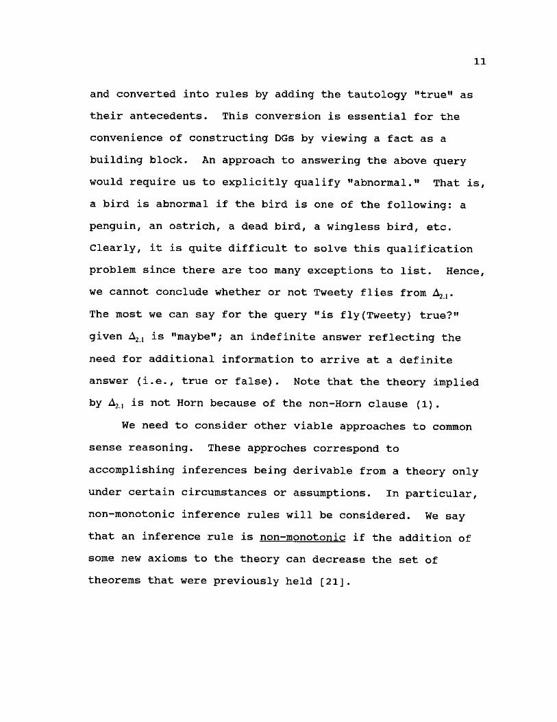
11

and converted into rules by adding the tautology "true" as

their antecedents. This conversion is essential for the

convenience of constructing DGs by viewing a fact as a

building block. An approach to answering the above query

would require us to explicitly qualify "abnormal." That is,

a bird is abnormal if the bird is one of the following: a

penguin, an ostrich, a dead bird, a wingless bird, etc.

Clearly, it is quite difficult to solve this qualification

problem since there are too many exceptions to list. Hence,

we cannot conclude whether or not Tweety flies from A^.

The most we can say for the query "is fly(Tweety) true?"

given is "maybe"; an indefinite answer reflecting the

need for additional information to arrive at a definite

answer (i.e., true or false). Note that the theory implied

by Aj! is not Horn because of the non-Horn clause (1).

We need to consider other viable approaches to common

sense reasoning. These approches correspond to

accomplishing inferences being derivable from a theory only

under certain circumstances or assumptions. In particular,

non-monotonic inference rules will be considered. We say

that an inference rule is non-monotonic if the addition of

some new axioms to the theory can decrease the set of

theorems that were previously held [21].

12

2.3 Non-monotonic Inference Rules for Processing

Negative Information

2.3.1 Negation as Failure Rule

The "negation as failure rule" (NF-rule) was developed

by Clark [2] and has been used to logically deduce negative

information [2, 21, 32-34].

Definition 2,1; Let T be a theory defined by a set of

axioms A. The NF-rule states that if a ground predicate q

is in the SLD finite failure set of A, then we infer the

ground negative literal --q.

The SLD-resolution augmented by the NF-rule is called

SLDNF-resolution. Following SLDNF-resolution, a predicate

in a goal can be selected for resolution; however, only a

ground negative literal in a goal can be selected, based on

the safeness consideration, for resolution. When a

predicate in a goal is selected, we use essentially SLD-

resolution to derive a new goal with bindings created by a

unification with some known information, such as a rule or

fact, in A; whereas, when a ground negative literal - q in a

goal is selected, an attempt is made to construct a separate

SLDNF-tree with the ground goal clause (<- q) as its root.

If this rooted tree yields an SLDNF-refutation as indicated

by the empty clause, then the root (<- q) is false or

equivalently, q is true; and the subgoal (< -q) selected

from its corresponding goal (i.e., the goal containing the

13

negative literal --q) fails which means that the subgoal

(•< -q) is true or equivalently, -•q is false. On the other

hand, if an SLDNF-refutation cannot be found in an SLDNF-

tree rooted at («- q), the goal is true or equivalently, q is

false; and the subgoal (<- --q) succeeds which means that the

subgoal («- --q) is false or equivalently, --q is true. Since

the selection of a negative literal --q in a goal is limited

to a ground one and bindings are never created (since -q is

ground and the success or failure of the subgoal (•< >q) is

determined by the SLDNF-tree rooted at (*- q)), the NF-rule

is only a test for success or failure as just discussed. If

G is a goal and at some point in a computation of A U {G} a

subsequent goal is reached which contains only non-ground

negative literals, then we say that the computation of A U

{G} flounders. In this case, no literal is available for

selection to satisfy the safeness condition. For example,

take A to be {p(X) <—'r(X)} and G to be («- p(X)). Then the

computation for A U {G} flounders. Since the SLD finite

failure set of A is a subset of the complement of the

success set of A, the NF-rule is non-monotonic.

Example 2.2: Referring to the set of axioms A^ in Example

2.1, can we infer "Tweety flies?"

The solution based on the NF-rule is shown in Fig. 1.

The SLDNF-tree rooted at the initial goal (•<- fly (Tweety)) is

shown in Fig. 1(a) in which the final goal (< -abnormal

(Tweety)) contains a ground negative literal. Thus, the

14

process proceeds by constructing a separate SLDNF-tree

rooted at the goal (<- abnormal(Tweety)), which is shown in

Fig. 1(b) where the last goal (•<- --fly(Tweety)) derives no

refutation and hence fails. This means that abnormal

(Tweety) is false or equivalently, -"-abnormal (Tweety) is true

which in turn implies that the final goal of Fig. 1(a)

succeeds. Thus, the root of Fig. 1(a) is false or

equivalently, fly(Tweety) is true.

«- fly (Tweety)

(1) {Tweety/Y}

*- bird (Tweety) A -abnormal(Tweety)

(3)

<- -abnormal (Tweety)

(a) SLDNF-tree rooted at («- fly (Tweety)) .

abnormal(Tweety)

(1 *) {Tweety/Y)}

bird(Tweety) A -fly(Tweety)

(3)

••fly (Tweety)

fails

(b) SLDNF-tree rooted at (*- abnormal (Tweety)) .

Fig. 1. SLDNF-trees for the query "Can Tweety fly?"

15

2.3.2 Herbrand Rule

Let T be a theory defined by a set of axioms A. The

Herbrand rule [21] requires that each predicate in A be

completed and to T an equality theory be augmented. There

are two cases to consider.

(1) The completion of each head predicate.

This is done by adding the necessary condition (only if

part) of the definition to the head predicate h along

with an equality theory to T. The completion of such a

predicate provides a technique for minimizing the

number of objects that satisfy the head predicate. The

completion of h for each clause

h(Y) +- bn A — A b^ (2.1a)

with i = 1, ..., k (i.e., h(Y) is defined by k > 1

alternative antecedents or bodies) and Y being a

sequence of Y1( ..., Yn of variables is defined as

COMP[A; h] = {VX h(X) « (body! V ... V bodyk) > (2.1b)

in which X is a sequence of universally quantified

variables Xlf ..., X„ not appearing in each original

clause (2.1a), VX abbreviates (VXlf ... VXJ , and body;

stands for the body of (2.1a) for each i = 1, ..., k.

Each such body; is written as the following normal form

(3W (X = Y) A bu A ... A b^)

where W is a sequence of existentially quantified

variables each appearing in some b for j = 1, ..., nij,

and (X = Y) abbreviates ((Xj = Yj) A ... A (X„ = Yn)) .

16

(2) A predicate symbol in A not appearing in the head of

any rule.

For each such predicate symbol, say, p(Wt, Wn.) , we

consider it as the clause

VW(p(Wj, ..., Wn.) «- false)

since p(Wlf Wn.) is neither a unit clause nor a

normal rule where false is a contradiction and W is a

sequence of universally quantified variables Wlf ...,

Wn.. Then we complete it as

VW(p(Wj, Wn.) 4* false)

which is equivalent to

VW ~'P(Wj, Wn.) . (2.1c)

An alternative explanation along the above line entails

the following. Since p(Wx, — , Wn.) is neither a unit

clause nor a normal rule, it can serve only as a

predicate in some goal of an SLDNF-tree. Hence, we can

select it to form the following subgoal

VW(*- p(Wx, . . Wn,))

which is equivalent to (2.1c).

Let COMP(A) denote the completion of A in which each

predicate p in A is completed. Since COMP(A) is stronger

than A, it is clear that COMP(A) •= A where the symbol "n"

(")M«) stands for "logically implies" ("does not logically

imply"). COMP(A) can be inconsistent for theories which are

not Horn. For example, if A = {p «- -p} which is non-Horn,

then COMP(A) = {p & --p} which is inconsistent since COMP(A)

17

i= p and COMP(A) •= -p. However, if T is Horn, then COMP(A)

is consistent. Predicate completion is non-monotonic.

Example 2.3: The completions of the predicates in are

as follows.

COMP(A21; bird) = {VX bird(X)

«=> ((X = Tweety) V (X = Jimmy)) >

where bird occurs positively only once in each clause of

A2.1t

COMPfAaj; fly) = {VX fly(X)

<=> 3W ((X = W) A bird(W) A --abnormal (W)) }

where fly occurs positively only once in (1) of A^,

COMPfA^; abnormal) = {VX abnormal(X)

3W ((X = W) A bird(W) A -fly(W))}.

The last completion is based on the clause (abnormal(Y) <-

bird(Y) A -"fly(Y)) which is equivalent to (1) in A^ where

abnormal occurs positively only once in the former

equivalent clause. Note that this completion does not help

us much for handling common sense situations. Intuitively,

what we would like is to conclude abnormal(X) <=» (X = Jimmy)

since Jimmy is a bird by (4) in A^ and Jimmy cannot fly by

(2) in A J J .

COMP(A) is consistent if A is solitary in each

predicate (i.e., each clause in A is solitary in p if the

clause having a positive occurrence of p has at most one

occurrence of p [10]). For example, is solitary in

bird, fly, or abnormal.

18

Definition 2.2; The Herbrand rule states that if a ground

predicate q is not a logical consequence of COMP(A), then we

infer -q.

If T is a Horn theory, then the Herbrand rule is more

powerful than the NF-rule [21]. However, we cannot complete

a predicate p to obtain a consistent COMP(A) if A is not

solitary in p because the completion process might produce

circular definitions for p, which would not restrict the

object constants that satisfy p to those that must do so,

given A.

2.3.3 Closed World Assumption

The "closed world assumption" (CWA) was developed by

Reiter [28]. It has been applied for resolving the

complement of a relation in a relational database in such a

way that any one tuple that is not explicitly in a relation

of the database is taken to be false or in the complement of

the relation.

Definition 2.3 [28]: Let T be a first-order theory defined

by a set of axioms A. The closed world assumption states

that if a ground predicate q is not a logical consequence of

A, then --q is logically implied by A. In other words,

CWA(A) = A U {-•q; q is a ground predicate and A *= q}. (2.2)

The CWA completes the theory T. A theory T is complete

if either every ground predicate in the language L or its

negation is in T [10]. The CWA is non-monotonic since the

19

set of augmented ground negative literals would shrink if we

added a new ground predicate to A.

A set of axioms is consistent if A has a model, and

inconsistent otherwise [21]. As proved in [10], the CWA(A)

is consistent iff for every clause B = Bx V ... V Bn, in

which each B; for i = 1, ..., n is a ground predicate,

(a) If A f B then

(b) A n= Bj for some i.

On the other hand, the CWA(A) is inconsistent if there

exists B as shown above such that

(a) A »= B, but

(b) A £ Bj for each i.

In particular, the CWA(A) is consistent if T is Horn and

consistent.

Consider the following example for illustrating the

case of inconsistency.

Example 2.4: Let A^ = {r(Cj) V r(C2), s(C3)}. Following

(2.2) in Definition 2.3 we have

CWA(A2.2) = A22 U {^(q) , -,r(C2), {C^), --sfC!), -"S(C2)}.

This completed set of axioms is inconsistent since both

(rfq) V r (C2)) and its negation (i.e., (-rrfCj) A -rr(C2))) in

the equivalent form of {-r(Cj) , -r(C2)} are in CWAfA^) where

a set means a conjunction. The source of this difficulty is

the existence of the indefinite ground predicates rfC^) and

r(C2) in the disjunction (r(Ci) V r(C2)).

20

Although the CWA is more powerful than the Herbrand

rule for a Horn theory and Horn theories have consistent CWA

augmentations [24], it is too strong to be flexible for many

applications and especially, Horn theories are in general

not adequate for common sense reasoning.

2.3.4. Generalized Closed World Assumption

Minker [24] removed the source of the CWA's difficulty

and developed the generalized CWA (GCWA) by adding an

additional constraint on each augmented ground negative

literal.

Definition 2.4 [26]: Let T be a first-order theory defined

by a set of axioms A without function symbols. The

generalized CWA applied to A is defined as follows:

GCWA (A) = A U {-"q: q is a ground predicate and there is

no ground clause B of predicates such that

A t= (q V B) , but A B}. (2.3)

Consider the theory A^ in Example 2.2 again. By (2.3)

in Definition 2.4, we have

GCWA(A2.2) = A22 U {-,r(C3), —

1 s(Cj) , _is(C2) }

which is consistent. To see that -"rfCj) is not in GCWA (A) ,

we view q as r(Ci) and B as r(C2) . Then A *= (rfCJ V r(C2))

since this disjunction is given in A, but A r(C2) .

Similarly, we can show that ^r(C2) is not in GCWA (A) .

The GCWA(A) allows common sense reasoning. For the

query "Can we infer r(C3)?" the answer would be "false,"

21

since --rfCj) in GCWA(AJ2) is true. However, for the query

"Can we infer rfCj)?" the answer would be "maybe," since not

only r(Cj) is not in GCWA(A22) but also TfCi) is not in

GCWAfA^) . This indicates that neither r(Ct) is true nor

-*r(Cj) is true. In addition, the disjunction (r(Cj) V r(C2))

in A22 indicates that rfCj might not be false since the

disjuction being true requires that at least one of the

predicates must be true. Thus, anything that is not false

or true is not necessarily true or false, respectively, and

the answer for the above query is "maybe."

2.3.5. Circumscription

Circumscription was developed by McCarthy [22, 23] and

is an inference rule of non-monotonic reasoning designed to

handle incomplete and negative information in common sense

reasoning systems.

Definition 2.5 [19]: Let T be a theory defined by a set of

axioms A. Let P = {pw ...,pm} be a set of predicate

symbols, Z == {zlf ..., zn} a set of predicate symbols

disjoint with P, and A(P, Z) a sentence in A. The symbols

from Z are called variables. The parallel circumscription

of P in A with variables from Z is the sentence

CIRC(A; P; Z) = A(P, Z) and there is no P' and Z*

such that (A(P', Z") A (P' < P)), (2.4)

where P' = {p , ..., and Z' = {z{, ..., zn'} are similar

to P and Z, respectively. In (2.4), (P« < P) is the

22

abbreviation for ((P' < P) A ->(P < P')) in which (P1 < P)

abbreviates (VX P'(X) => P(X)). In addition, (P1 (X) => P(X))

stands for the conjunction of (Pi'(X) => P;(X)) for all i = 1,

. .., m.

The formula of (2.4) states that P has a minimal

possible extension under the assumption that A(P, Z) is true

when extensions from Z are allowed to vary in the process of

minimization [19, 22]. If p(tx, ..., tn) is an n-ary

predicate with symbol p and terms (tlf ..., tn) , then the

extension of p corresponds to the set of tuples that make

the predicate p(t1# ..., tn) true [22, 23]. In applications,

A(P, Z) is the conjunction of axioms, P is the set of

abnormality predicate symbols, and Z is the set of symbols

that are to be characterized with the circumscription [19].

Intuitively, circumscription states that objects

satisfy a given predicate only if they must.

Circumscription may also be defined in model-theoretic

terms.

Definition 2.6 [19, 22]: Let A, T, P, and Z be defined as

shown in Definition 2.5. For any two models M and N of A,

we write (M <P;Z N) if M and N differ only in how they

interpret the predicate symbols in P and the predicate

symbols in Z, and the extension of every predicate symbol

from P in H is a subset of its extension of every predicate

symbol from P in N. A model M of A is minimal with respect

to <P;Z if there is no model N of A such that (N <P;Z M) .

23

Observe that negative literals are minimized by not

appearing in a model. Moreover, since we minimize positive

literals by not only minimizing positive literals but also

maximizing negative literals, only positive literals need to

appear in a model. Thus, a negative literal --W is derived

from a model M if W is not in M.

Note also that a minimal model of A with respect to <P;Z

is, in general, not equivalent to the concept of minimal

models as defined in [21], in which a model M of A is

minimal if thesre is no other model M1 of A where the arity

of M1 is less than the arity of M. In the special case in

which M is the unique minimal model of A with respect to

<P;Z, M is also a minimal model of A in the sense of [21].

Proposition 2.1 [19, 22]: A structure M is a model of

CIRC(A;P;Z) iff M is a minimal model of A with respect to

<P;Z. That is, for any formula F, CIRC(A;P;Z) logically

implies F iff M logically implies F for every minimal model

M of A with respect to <P;Z.

A generalization to the above parallel circumscription,

namely the formula circumscription, is proposed by McCarthy

[23]. Formula circumscription applies not only to ground

predicates but also to predicates with variable arguments

and second order well-formed formulas. Formula

circumscription is beyond the scope of this investigation.

Example 2.5:: Let A^ be the set of axioms as shown in

Example 2.1., From such axioms, we should conclude that

24

Tweety can fly since there is no information that Tweety is

abnormal. Let P = {abnormal} and Z = {fly}. Then we have

CIRC(Aa.j; P; Z) = VX (abnormal(X) iff X = Jimmy),

from which fly(Tweety) is logically implied.

A solution based on the model-theoretic terms of

Definition 2.6 can also be found. For this, assume that

satisfies the domain-closure axiom (DCA). The DCA [10, 29]

says that the only elements in the underlying domain are

those that can be named using the constants and function

symbols in a first-order language L. Let tlf t2, ... be all

the constants in L and X be a variable. If there are no

function symbols in the language, the DCA can be represented

by

VX (X = tx) V (X = t2) V ...

where the t} are the constants used to name a specific

element in the underlying domain. With this, has only

two models Mj and M2 where Mx = {bird(Tweety), bird(Jimmy),

abnormal(Jimmy), fly(Tweety)}, and M2 = {bird(Tweety),

bird(Jimmy), abnorma1(Jimmy), abnorma1(Tweety)}. However,

only Mx is a minimal model of with respect to <P;Z. In

effect, Mx and M2 differ only in how they interpret the

predicate symbols in P and those in Z, and the extension of

the predicate symbol abnormal in Mj (i.e., {Jimmy}) is a

subset of the extension of abnormal in M2 (i.e., {Jimmy,

Tweety}). Thus, by Proposition 2.1 and with being the

25

only minimal model of A^ with respect to <P;Z, both

abnormal(Jimmy) and fly(Tweety) are logically implied.

If circumscription is applied to two or more

abnormality predicate symbols PjS in P, the result may

depend on the order in which the P;S are circumscribed.

Therefore, it is desirable to assign different priorities to

the P;S. Prioritized circumscription formalizes these

cases.

Definition 2.7 [19, 20, 23, 27]: The prioritized

circumscription of A with the priorities Pj > ... > Pk and

variables from Z is denoted by

CIRC (A; Pj > ... > Pk; Z) = CIRC (A; P;,- {Pi+1 U ... U Pk U Z})

A ... A CIRC(A; Pk; Z), for i = 1, ..., k-1. (2.5)

Example 2.6 [8]: Let A^ = VX (Pj(X) V P2(X)) . Then

CIRC(A23; Pt; P2) = VX (Pi(X) «• -P2(X)).

CIRC(A23; P, > P2; <p ) = VX (-P,(X) A P2(X)).

Circumscription has been thoroughly studied in the

literature, and its power as a non-monotonic inference rule

is well supported. However, its major drawback is that it

is very expensive to compute [19]. Indeed, the definition

of circumscription involves a second-order formula since the

quantification is applied to predicate symbols. Although

Lifschitz [19] showed some cases in which computing

circumscription reduces to a problem in first-order logic,

the trouble remains in the general case.

26

2.3.6. Extended Closed World Assumption

The extended CWA (ECWA), developed by Gelfond et al.

[9], is equivalent to the first-order version of McCarthy's

circumscription for function-free theories satisfying also

the DCA and the UNA, and subsumes both the CWA and the GCWA.

The DCA and the UNA assumptions allow us to reduce A to a

propositional combination of ground atoms and prohibit the

use of synonyms in our language.

Definition 2.8 [9]: Let T, defined by a set of axioms A, be

a function-free theory satisfying also the DCA and the UNA.

Let P and Z be defined as shown in Definition 2.5. Let Q be

the set of all predicate symbols in A, but not in P U Z.

Let P+ be the set of predicate symbols of positive literals

with symbols in P. We say that an arbitrary sentence K

involving only predicate symbols in P+ U Q is free for

negation (FFN) in A if there exists no disjunction B = B! V

... V Bn where the symbol of each B; is in P+ U Q such that

(i) A .= (K V B) ,

but

(ii) A M /

where the disjunction (K V B) is minimal in A. This

minimality means that (K V B) is logically implied by A, but

not subsumed by any other disjunction logically implied by

A. On the other hand, if there exists such a B to satisfy

both conditions (i) and (ii), then K is not FFN in A.

27

By this definition if K is FFN in A, then "-K is true"

or equivalently, "K is false." On the other hand, if K is

not FFN in A, then (i) either "K is true" if A t- K or (ii)

"K is maybe" if A K.

Definition 2.9 [9]: Let A, T, P, and Z be defined as shown

in Definition 2.5. The ECWA with respect to P and Z applied

to A results in the following closure:

ECWA(A; P; Z) = A U {-K: K is FFN in A}. (2.6)

Example 2.7; This example shows that the negation of an FFN

sentence in A is true. Consider the set of axioms A21 as

shown in Example 2.1. Let P = {abnormal} and Z = {fly}.

Assume that the DCA holds. Then we have Q = {bird}. We

show that the predicate abnormal(Tweety) is FFN. Indeed,

rewriting (1) and (2) in A21 as

(l1) -•bird(Y) V abnormal(Y) V fly(Y) ,

(2') -bird(Jimmy) V -fly(Jimmy),

we see that the only disjunction derivable from A^ with K =

abnormal(Tweety) in the disjunction is the instance of (11)

by the unifier {Tweety/Y} [21]; i.e.,

(II) {Tweety/Y} -•bird (Tweety) V abnormal (Tweety) V

fly(Tweety).

This instance is not minimal, but

(III) abnormal(Tweety) V fly(Tweety)

is minimal since -bird(Tweety) in the instance

(11){Tweety/Y} is false because of the existence of (3)

(i.e., bird (Tweety) «- true) in A2j. Hence, fly(Tweety)

28

corresponds to B in Definition 2.8, i.e., B = fly(Tweety).

Since the predicate symbol abnormal of K = abnormal(Tweety)

is in P+ (and also in P+ U Q) and the predicate symbol fly

of B = fly(Tweety) is not in P+ U Q, abnormal(Tweety) is FFN

in A^, which means that --abnormal(Tweety) is true. Now it

is easy to see that with Y replaced by Tweety, the body or

antecedent (i.e., bird (Tweety) A --abnormal (Tweety)) of the

instance (1){Tweety/Y} is true and so is the head or

consequent. That is, B = fly(Tweety) is true.

As mentioned above, Gelfond et al. [9] show that the

CWA and the GCWA are special cases of the ECWA, and that the

ECWA is equiveilent to the first-order version of

circumscription for function-free theories T satisfying also

the DCA and the UNA. The ECWA is also equivalent to

prioritized circumscription if T is also a stratified theory

[9]. The foregoing equivalence together with the fact that

the ECWA is computationally more efficient [9, 19, 29] make

the ECWA a good alternative to develop an inference

algorithm for common sense reasoning. The following theorem

is the cornerstone for a proof that the first-order version

of circumscription is equivalent to the ECWA.

Theorem 2.1 [ 9 ]: A sentence K is FFN in A iff M i= -OK for

every minimal model M of A with respect to <P;Z.

The consistency of the ECWA is summarized in the

following corollary.

29

Corollary 2•1 [9]: If A is consistent, then so is ECWA(A;

P; Z).

It has been shown [9] that in the case of stratified

theories (as will be defined) the iterated CWA (ICWA) is

equivalent to the prioritized circumscription. For defining

these notions, we call a theory T, defined by a set of

axioms A, disjunctive over a language L if A consists of a

finite set of clauses of the following form

Cx V . . . . V Ck <- A j A ...A A , A - B , A . . . A -B„ (2.7)

where m, n > 0, k > 1, and A , Bjf and C, are predicates. A

stratified theory and the ICWA aire defined as follows.

Definition 2.10 [36]: We say that a disjunctive theory T is

stratified if, for a given set S of all predicates in a

language L, it is possible to partition S into disjoint sets

Sj, ..., Sr (i.e., a stratification of T) in such a way that

for each clause of the form (2.7) in A there is a constant c

with 1 < c < r such that

(a) Stratum(Cj) = Stratum(Cj) = c, for each i, j;

(b) Stratum(AJ < c, for each i; and

(c) Stratum(BJ < c, for each i

in which the Stratum of a predicate symbol in Sj is equal to

i.

Consider a stratified disjunctive theory T over the

language L with the stratification Su Sr as partitioned

from S. Let P and Z be as shown in Definition 2.5. Let Ln

be the language consisting of all constants of L and of all

30

predicate symbols from Qn+ = U {Sj | j < n}. Let Tn be a

theory over L„ and defined by a set of axioms \ consisting

of all clauses from A that define predicates from Qn+. That

is, only predicates from Q„+ belong to the conclusions of

these clauses. It is easy to see that A = Ak and L = 1^.

Let Pn+ = P + n S„ and Z„+ = Z+ n Qn. Then the ICWA is defined

as follows.

Definition 2.11 [36]: The ICWA applied to A results in the

closure ICWAfA/Pj > ... > Pk;Z) for 1 < k < n:

ICWA(A1;P1;Zx) = ECWAfAi/PjfZi) , (2.8a)

ICWA(An+1;Pl > ... > Pn+1;Zn+1) = ECWA(A„+1 U

ICWA(AQ^PJ > ... > Pn;Zn) ,Pn+i7Zn+1) , n > 0. (2.8b)

2.4. Default Reasoning

Default logic is an approach to dealing with incomplete

information by allowing a first-order theory T to be

augmented with new inference rules provided that some

premises or axioms are satisfied.

Definition 2.12 [6, 30]: A default theory is an ordered

pair (D, W) consisting of a set of first-order formulas W

and a set of defaults D. A default is an expression of the

form:

A (X) -.MiB^X) A ... A Bm(X) ) ( 2 . 9 )

C(X)

where the prerequisite A(X) , the joint justifications Bj(X)

for each j == 1, ..., m, and the consequent C(X) are all

31

formulas with the free occurrences of their variables among

those in X = [Xl7 X,,}, and M is read as "it is

consistent to assume."

Intuitively, (2.9) means that we may believe the

consequent, C(X), so long as the prerequisite, A(X), holds

and the joint justifications, Bj(X) for each j = 1, ..., m,

remain consistent (i.e., --Bj is not provable from the

underlying default theory for each j = 1, ..., m). In some

cases, the prerequisite A(X) in (2.9) may be absent. We say

that a default is closed if A, Eij for each j = 1, .. ., m,

and C contain no free occurrences of variables; otherwise,

we say that the default is open. If the default has only

one justification, say B(X), then we say that such default

is normal if B(X) = C(X), and we say that it is semi-normal

if B(X) = C(X) A U(X) for some U(X) [6, 7].

Definition 2.13 [6, 30]: Let (D, W) be a default theory.

In terms of fixed points, we say that E is an extension of

(D, W) if it is a least fixed point (lfp) of an operator

(Th) with the following characteristics.

(1) W C E.

(2) lfp (Th (E)) = E.

A :M(BX A ... A Bm) (3) Every default C D,

C

if A is in E, and --Bj for each j = 1, .. ., m is not in

E, then C is in E.

32

Informally, E is the set of conclusions derived by (D, W)

and Th(E) the set of theorems provable from E. In other

words, E includes all known information and the consequent C

of any default if the prerequisite A is satisfied and the

joint justifications BjS are all consistent in E.

Example 2.8 [30]: Consider the following default theory

(2.4/ ^2.4) •

:M(--block (A)) D24: ,

-block(A)

:M(-block(B))

-block(B)

W24: block(A) V block(B).

Then, Ej and E2 are the only extensions (i.e., answer sets)

of (D24, W24) , where E! = {-block(A) , block(B)}, and E2 =

{block(A), -block(B)}. Observe that this outcome is

consistent with the CWA. However, Example 2.9 below shows

that there are theories that do not have extensions.

Example 2.9 [30]: Consider the following default theory

(12.5/ •

:M(A) 2.5 • •

-A

W25: 0 (i.e., the null formula).

Example 2.10: Consider the following example of an default

theory (D2.6, W2.6) .

2.6

33

:M(fly (X) «- bird(X))

fly(X) «- bird(X)

W26: bird(X) <- penguin(X) V dead-bird(X) V ostrich(X) ,

-fly(X) <- penguin(X) V dead-bird(X) V ostrich(X),

bird(Tweety) <- true.

Since we cannot infer whether or not Tweety flies from W26,

we may use D26, in conjunction with W26, and infer that

"Tweety flies1" is true by default.

Imielinski [15] argues that for some W = {black

(Tweety)},

bird(X) :M(fly(X)) Dl ;

fly(X)

is not equivalent to D26 since, he says, "if we do not know

whether Tweety is a bird, then we do not want to conclude

that if Tweety is a bird, then it would fly, since Tweety

may turn out to be not a typical bird." While such a

distinction is valid, D26 and D' can be regarded as

equivalent since an answer is computed based only on the

information at hand.

In general, if (2.9) is assumed at some point, it must

be retracted if at some other point some Bj becomes

inconsistent as a result of considering other defaults. The

following example shows that these inconsistencies can occur

if we have interacting defaults.

Example 2.11 [7]: Consider the following problem of

interacting defaults: Typical adults are employed; typical

34

high-school dropouts are adults; and typical high-school

dropouts are not employed.

adult(X) :M(employed(X)) D27: (1) ,

employed(X)

dropout(X) :M(adult(X)) ( 2 ) f

adult(X)

dropout(X) :M(-'employed(X)) (3)

-•employed (X)

Then if we know that someone is a dropout, we could assume

that he is an adult and not employed, i.e., by (2) and (3).

However, such result would be ambiguous since typical adults

are employed, i.e., by (1). The inconsistency problem that

could arise from multiple interacting defaults is analogous

to the problem of minimizing multiple abnormality predicate

symbols in circumscription. In this case we need to

consider prioritized circumscription.

The above ambiguities can be resolved by, for example,

using semi-normal defaults [7].

adult(X) : M(employed(X) A -'dropout(X)) D2.7: (1) -,

employed(X)

dropout(X) : M(adult(X))

adult(X)

dropout(X) : M(-employed(X))

-employed(X)

Clearly, this solves the foregoing problem since now we

cannot use (1) after using (2) and (3). However, the use of

35

semi-normal defaults has some disadvantages [7]: (1) The

theory becomes more complex; (2) the defaults may

overrestrict the interactions among themselves and as a

result, the theory may become contradictory; and (3) the

interactions must be explicitly known at the time of

inference.

Etherington [6, 7] has also investigated the

inconsistency problem of multiple defaults. Specifically,

he defines an ordering for semi-normal defaults and proves

that if a defciult theory (D, W) has such ordering, then it

is consistent (i.e., it has an extension).

Definition 2.14 [6, 7]: A semi-normal default theory is

ordered iff there is no literal A such that A « A, where

the symbol M « M and the subsequent symbol H<<" stand for

partial relations on the Cartesian product {literals} x

{literals}, for a closed semi-normal default theory (D, W).

These relations are defined as follows.

(1) If A is in W, then A = (A, V ... V AJ , for some n > 1.

For each AJ, Ak in {Alf ..., AJ, if A, * Ak, then let -AJ

<< Ak.

A :M(B A C) (2) If H is in D, then H .

B

Let Aj, . „., Aj, Bj, ..., Bs, and Clf ..., ct be the

literals of the clausal forms of A, B, and C,

respectively. Then

(a) If A.| is in {Aj, ..., AJ and Bk is in {Bj, , BJ,

36

then let Aj << Bk.

(b) If Cj is in {Cj, ..., Ct} and Bk is in {Bj, ..., BJ,

then let -q « Bk.

(c) Also, B = (Bj, Bm), for some 1 < m < s. For

each j < m, Bj = (B^ V ... V Bjmj), where mj > 1.

Thus if Bjk/ Bjp are in {Bu, ..., Bminm} and Bjk ^ Bjp

then let -Bj>k << Bjp.

(3) The expected transitivity relationships hold for « and

<<. That is,

(a) If A << B and B << C, then A << C.

(b) If A << B and B « C, then A << C.

(c) If A << B and B << C, or A << B and B « C, then A

« C.

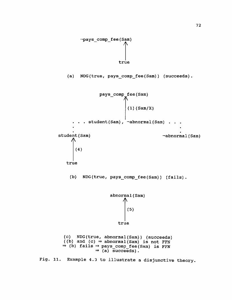
Example 2.12 [7]: Consider the following default theory

( 2.8/ 2.i) *

:M(A A -B) 2.8* ( -) I

A

:M(B A -D) ( 2) ,

B

:M( (D +- C) A -A) ( 3 )

D <- C

2.8 • '

Then we have {B « A}, {D « B}, and {C << D, ->D << -C, A «

"•C, A « D} respectively from (1), (2), and (3). Therefore,

(°2.8/ w2.8> i s n o t ordered since B « A, C « B, and A « C

imply A « A.

37

Effectively, Etherington's ordering solution to the

multiple defaults problem is analogous to the stratification

solution to the case of prioritized circumscription.

2.5. Deduction Graphs

A deduction graph (DG) is a powerful inference tool

which allows us to make inferences in Horn theories.

Application domains include the following:

(1) DGs were used to provide requisite results which are

yielded by the removal of extraneous attributes,

redundancies, and superfluities for designing a better

relational database scheme [38, 39, 42].

(2) DGs were participated in developing a rule base of an

expert system [13, 31] or an intensional database of a

deductive database [25] with the properties of

independence, completeness, consistency, and

nonredundancy [38-42].

(3) DGs can be applied for proving theorems since the set

of rules corresponding to the set of full arcs in a DG

forms a proof and the Horn formula (HF) derived by the

foregoing set corresponds to a theorem [21].

(4) Processing a database query [38-42] and evaluating

logic queries in a deductive database [25], rule-based

expert system [13], or logic programming system [21]

can be solved by DGs and particularly minimum DGs [14,

42].

38

Definition 2.15 [14, 40, 42]: A DG from its starting node

called source to its ending node called sink, denoted by

DG(source, sink), is a single entry and single exit,

connected, acyclic graph consisting of a set of simple

and/or compound nodes and a set of full and/or dotted arcs

such that the following conditions are satisfied.

(1) Source is the single entry (without incoming full arcs)

and sink is the single exit (without outgoing full

arcs).

(2) A simple node is defined by a predicate (or true if

source = true where true is a tautology).

(3) A compound node is defined by a conjunction of at least

two predicates.

(4) A full arc is defined by a rule from the body of the

rule to the head of the rule (where a rule means a

given headed Horn clause (HC), the instance of some

rule by a unifier, a unit clause representing a base

predicate corresponding to a relation scheme, and a

fact).

(5) A dotted arc is defined by connecting a superset of

predicates to one of its nonempty subsets (where a set

means a conjunction).

(6) Except the source with jsource| = 1 or each component

of the source with |source| > 1, there is exactly one

full arc incident to a simple node.

Note that a fact in condition (4) is a ground unit

39

clause and each unit clause is aiugmented by the body "true"

and viewed as a rule to be served as a building block for

constructing a DG. The formula (sink «- source) is derivable

from the conjunction of the rules corresponding to the full

arcs in a DG(source, sink). The formula (sink «- source) is

a rule or an HF where the latter will be defined.

In the above definition, a set of predicates

corresponds to a conjunction. A node is simple if it

corresponds to a predicate (including the tautology "true"),

and is compound if it is a conjunction of at least two

predicates. A DG as defined in Definition 2.15 is of and-

type and referred to as an and-DG.

An HF of the form (sink <- source) satisfies the

following conditions [14, 40, 42]:

(1) An HC is a degenerate version of an HF.

(2) The sink is a conjunction of predicates excluding true.

2.5.1 Deduction Graphs of And-type

Let R be a set of rules, s be a starting node, and t be

an ending node. Let i = {ix, ..., in} be the intersection of

s and t, and d = s - t = {dlf d,,,} be the difference of

s and t where n, m > 0. The case in which n = 0 or m = 0

means i = <f> or d = <pt where 0 denotes the empty set.

Suppose the HF of the form

t «- s (2.10)

is provable from (the conjunction of the rules in) Rj i.e.,

40

Re H t «- S (2.11)

where R<. consists of some rules of R, and possibly the

instances of some rules in R by unifications and some facts

in the underlying database. It was proved in the literature

[40-42] that Rc is structured as a DG from s to t. With the

inference rules of reflexivity, transitivity, and

conjunction for HFs, DGs of the and-type can be classified

into the following three classes based on their inference

functions.

(a) The general configuration

A

1" * * * <^m

s s (i) (ii)

V s

(iii)

1 • dj ... ^ . dj

s (V)

(b) The specific configurations

Fig. 2. Configurations of trivial DG, TDG(s, t) ((b.i)), and redundant DGs, RDG(s, t)s ((b.ii) through (b.v)).

41

Fig. 2(a) shows the general configuration of the

trivial and redundant DGs from s to t. Under different

conditions, this general configuration is differentiated

into five specific cases as shown in Fig. 2(b).

1) Trivial DGs: (Fig. 2(b.i))

A DG from s to t, denoted by TDG(s, t), and the

corresponding inference accomplished by (2.11) are both

called trivial if the HF of the form (2.10) being provable

from Rc is trivial. That is, this HF is trivial if t is a

nonempty subset of s. In this case, Rp is the empty set <p

corresponding to the empty conjunction with the truth value

true.

2) Redudant DGs: (Fig. 2(bii) through 2(b.v))

A DG from s to t, denoted by RDG(s, t), and the

corresponding inference accomplished by (2.11) are both

called redundant if each rule decomposed from the HF of the

form (2.10) being provable from Rc is also included in Rc.

Note that if an HF is of the form (hjfXj), ..., hk(Xk) <- body)

where X; is a sequence of arguments of the predicate hif then

each rule of the form (h;(Xj) «- body) for 1 < i < k is called

a decomposed rule from the HF. Fig. 2(b.ii) exists if i =

0, m = 1, and (t «- s) is in Rc. Fig. 2(b.iii) exists if i =

0, m > 1, and (dj «- s) for each 1 < j < m is in Rc. Fig.

2 (b. iv) exists if s = i, n > 0, m > 0, and (dj <- s) for each

1 < j < m is in Rj. Fig. 2(b.v) exists i f s ^ i , n > 0 , m >

0, and (dj <- s) for each 1 < j < m is in R,..

42

3) Nonredundant DGs: (Fig. 3)

A DG from s to t, denoted by DG(s, t), and the

corresponding inference accomplished by (2.11) are both

called nonredundant if it is none of the above two cases.

In this case, the general configurations are shown in Fig.

3. When t is simple, if a full arc (k, t) and a TDG(s, k),

1-A

TDGr^v RDG, or A DG from J s to k y

Fig. 3. Configurations of nonredundant DG, DG(s, t)s.

RDG(s, k) or DG(s, k) both exist, then DG(s, t) of Fig. 3(a)

is nonredundant. When t is compound, Fig. 3(b) is

nonredundant if at least one DG from s to dj for 1 < j < m

is nonredundant. Under different conditions, Fig. 3(b) can

be differentiated into three specific cases which are the

generalizations of Fig. 2(b.iii) through 2(b.v).

2.6. Deduction Graphs and other Inferencina Methods

We can use DGs to simulate the inference rule of modus

ponens in the case of predicates. Let p and q be

predicates. The inference rule of modus ponens states that

q is derivable from p and (p -*• q) ; i.e., {p, p -*• q} i— q. By

43

means of DGs, we first convert p into (p «- true) and then

use the alternative form q *- p and apply the inference rule

of transitivity for (q <- p) and (p <- true) to define the

DG(true, q) which derives (q «- true) .

In terms of expressive power SLD-resolution (and also

the generalized resolution [1]) is more powerful than DGs,

since SLD-resolution allows a non-Horn clause with negative

literals in the body of the clause while DGs allow only

rules as building blocks. However, SLD-resolution cannot be

used to express totally negative information using negative

clauses [32, 34] (a negative clause is equivalent to a goal

clause). Moreover, we can never infer negative information

using SLD-resolution directly, but only indirectly as a

result of some assumption (i.e., the NF-rule). It has also

been shown that SLD-resolution is not complete [34]. The

generalized resolution has the most expressive power, but it

is only refutation complete [10] and does not lend itself

well to the implementation of default reasoning [26].

2.7 Related Work

Recently, two algorithms related to implementing the

ECWA have been published [8, 27]. Both of these algorithms

are based on the concept of FFN sentences [8, 27], but have

conceptual and computational differences. Przymusinski*s

algorithm [27] is based on what he calls the MILO-resolution

which is a modification of the ordered resolution to build

44

the tree of a proof. To determine whether the ground

sentence ^ which has no function symbols follows from the

ECWA in a set of axioms A, the algorithm must prove that for

each sentence ip such that ^ «- <p, ^ is an FFN sentence. The

major drawback of the algorithm is that it is based on

ordered resolution which is not refutation complete [9].

Gelfond and Przymusinska1s algorithm t 8 3 / on the other

hand, implements a special case of the ECWA which he calls

"careful closure procedure" (CCWA) and works on a set of

axioms A composed of Horn clauses and non-Horn clauses of

the form (Alf ..., AN -»• Bt V ... V BK) where each A;, Bj is an

atom, and other restrictions on A are specified in [8]. To

determine whether a ground literal \j/ follows from the CCWA

in A, the algorithm must first decompose A into a set of

Horn As (AHs) and then infer \p if and only if each AH I— \f/.

The CCWA is sufficient for solving many common sense

reasoning problems [8]. However, the computational expense

of performing the decomposition of a non-Horn A to Horn As

and the checking of AH h- \p for each AH is very limiting. In

effect, for A with n non-Horn clauses with n; positive

literals in the i-th non-Horn clause we have to split A into

nn; different AHs. Moreover, Gelfond's approach is sound,

but not complete [27].

Yahya and Henschen's propose an approach [37] which is

more restrictive than the ones above. They consider A to be

a set of Horn and non-Horn clauses and implement an

45

extention of the GCWA by considering ^ to be a ground

positive clause instead of a ground predicate as in the

GCWA. However, like Gelfond and Przymusinska's algorithm,

the approach is also based on splitting A into AHs. Hence,

it also seems impractical.

With respect to default reeisoning systems, they have

been implemented mainly by using ATMS (Assumption Truth

Maintenance Systems) developed by de Kleer [3, 4]. The ATMS

approach exhausts all the possible worlds for some datum,

i.e., a literal, with a datura proved true if it is true in

all possible worlds.

Delgrande's approach [5] to default reasoning is based

on an extension to classical first-order logic.

Specifically, he augments first-order logic with an operator

"=>" for representing default statements. The statement (a

=> /3) is read as "if a then normally /3." The main advantage

of Delgrande's approach is the ability to reason about

defaults. However, his approach is not readily implemented

with available inference rules including modus ponens and

resolution because of his deviation from first-order logic.

2.8. Problem Statement and Proposed Solution

From the above discussions, the problem can be stated

as the need for a powerful formalization of common sense

knowledge with the ability to handle negative and incomplete

information. The proposed solution involves three parts.

46

First, the extention of deduction graphs, which yields a

powerful tool for deriving function-free Horn formulas, to

normal deduction graphs (NDGs) with the ability to derive

not only Horn but also non-Horn function-free formulas.

Second, the formalization of the CWA, the GCWA, and the ECWA

are all reformulated in terms of NDGs. Thus the ability to

handle negative information can be achieved. Third, the

default reasoning is also reformulated by means of NDGs to

provide the ability to handle incomplete information.

CHAPTER III

EXTENDING DEDUCTION GRAPHS TO NORMAL DEDUCTION GRAPHS

3.1 Introduction

In this chapter, deduction graphs (DGs), which form a

powerful tool for deriving function-free Horn formulas are

extended, to normal deduction graphs (NDGs) with the ability

to derive not only Horn but also non-Horn function-free

formulas. After formalizing NDGs, the information that NDGs

provide is consistent with Kleene's three-valued logic. The

inference provided by NDGs (including DGs) is compared with

resolution (including SLD-resolution, i.e., Linear

resolution with Selection function for Definite clauses) in

terms of expressive power. NDGs are shown to be more

powerful than the SLD-resolution. Also, one step in the

inference rule of resolution is simulated by means of NDGs

to suggest that a completeness proof for NDGs may be

possible if the resolution can be simulated by NDGs.

Lastly, the soundness of NDGs is proved. Several examples

are used to illustrate the above notions.

3.2 Normal Deduction Graphs

DGs are being extended to NDGs for accomplishing the

inference of a non-Horn function-free formula of the form (h

<- b) where b and h are conjunctions of function-free

47

48

literals or b can be the tautology "true." The building

block for constructing an NDG includes not only a rule (as

stated in condition (4) of Definition 2.15), but also a rule

that is accordingly modified in such a way that its head is

a literal and its body is a conjunction of literals. A DG

or rule in the foregoing extended version is called an NDG

or a normal rule, respectively.

Definition 3.1: Let R be a given set of rules and/or normal

rules. An MDG(b, h) derives a non-Horn formula (h <- b)

where b and h are conjunctions of function-free literals or

b can be the tautology "true." NDGs are constructed from

the superset R' of R constructed by augmenting R with rules

Rjk that result from every possible transformation of a rule

Rj into an equivalent rule containing a single literal as

its head and a conjunction of literals or true as its body.

Note that, according to Definition 3.1, the case where

h is a disjunction of literals (i.e., in (h «- b)) is not

defined. However, this case can always be transformed into

an equivalent one (i.e., (h' - b•)) where h» and b' are

defined as in Definition 3.1. With this understanding, an

NDG(b, h) where h is a disjunction of literals is also

defined.

Example 3.1; If R = {block(A) V block(B) - true}, then R' =

{block(A) <- --block(B), block(B) «- -block(A)}. Can we infer

"block(A) V block(B)?" Note that this problem cannot be

49

solved by means of DGs since R contains a non-Horn clause;

whereas by using NDGs, it can simply be solved by

constructing either an NDG (--block (A) , block(B)) or an

NDG(--block(B), block(A)) as shown in Fig. 4.

block(B) <- -•block (A)

Fig. 4. NDG (--block (A) , block(B)) (succeeds).

Now, we elaborate on the information that NDGs provide,

and show how such information is consistent with Kleene's

three-valued logic [16]. Fig. 5 shows the tables concerning

five three-valued logic operators where t, f, and m stand

for true, false, and maybe, respectively.

Q 7-Q V R t f m A

R t f m =>

R t f m <=»

R t f m

t f Q t t t t Q t t f m Q t t f m Q t t f m f t f t f m f f f f f t t t f f t m m m m t m m m m f m m t m m m m m m

Fig. 5. Three-valued logic operators.

Theorem 3.1: Let true and h be respectively the starting

and the ending node of an NDG(true, h) being constructed.

(a) If the construction of an NDG(true, h) succeeds, then

(h «- true) is derived from the NDG. In this case, we

infer that h is true or equivalently, -h is false.

(b) If the construction of an NDG(true, -h) succeeds, then

(-h «- true) is derived from the NDG. In this case, we

infer that --h is true or equivalently, h is false.

50

(c) If both (a) and (b) do not hold, then (h <- true) and

(-•h <- true) are both not derived from NDGs. In this

case, neither h is true nor -•h is true, and we infer

that h is maybe.

Note that it is impossible to have the case in which

both (a) and (b) hold since the underlying first-order

theory is assumed to be consistent.

Proof:

(a) This is a consequence of Definition 2.15. In

particular, a consistent first-order theory guarantees

that if "h is true," then "-•h is false." It can be

shown that the conjunction of the rules and/or normal

rules corresponding to the arcs in the NDG derives

(h *- true) , based on the inference rules of

reflexivity, transitivity, and union.

(b) This is the dual of (a).

(c) If the construction of an NDG(true, h) and that of an

NDG (true, -h) both fail, then both rules (h «- true) and

(-•h •<- true) are "not true" where "not true" does not

mean "-'true," but "false V maybe." It can be shown by

three-valued logic that we can only infer "h is maybe."

By -—table of Fig. 5, -•h is also "maybe."

Example 3.2: Consider the set of rules R from Example 3.1.

Can we infer block(B)? To infer block(B) we try to

construct an NDG(truef block(B)).,

51

block (B) -'block (A) true

Fig. 6. NDG(true, block(B)) (fails).

Fig. 6 shows that the construction of an NDG(true,

block(B)) fails at node --block(A) . An NDG(true, -•block(B))

fails immediately since no rule unifies with -•block (B) .

Hence, for block(B) we conclude "maybe" by Theorem 3.1(c).

3.3. Normal Deduction Graphs and Resolution

In this section, the differences between NDGs

(including DGs as a special case) and resolution (including

SLD-resolution) are examined in terms of their expressive

power and completeness. The reader is referred to [14, 26,

40, 42] for more details on DGs including their advantages

when compared to other inferencing methods, and to [21] for

more details on SLD-resolution.

It is clear that in terms of expressive power SLD-

resolution is more powerful than DGs, since SLD-resolution

allows the use of a non-Horn clause, whereas, DGs allow only

HCs as building blocks. By the same token, SLD-resolution

is less powerful than NDGs since NDGs allow normal rules as

building blocks including not only zero or more negative

literals in the body of a normal rule but also zero or more

negative literals in the head of a normal rule. Thus, it is

possible to express totally negative information using

negative clauses [34] (a negative clause is equivalent to a

52

goal clause) using NDGs, while with SLD-resolution it is

not. Moreover, using NDGs we can infer negative information

directly, while using SLD-resolution only indirectly as a

result of some assumption (i.e., the NF-rule).

Example 3.3; Given R = {-A «- B, A «- true}, can we infer --B?

With R' = {--"A «- B, A •- true, -B <- A} which is a superset of

R, Fig. 7 shows that an NDG(true, -*B) succeeds. Thus, we

infer "-B is true." Observe that we cannot solve this

problem using SLD-resolution since the head (--A) of the rule

(-A «- B) in R is not an atom. Moreover, it has been shown

that SLD-resolution is not complete [34].

-•B A ^ true

Fig. 7. NDG(true, --B) (succeeds).

Example 3.4: Let R = {A <- B, A <- -B}. It can be shown that

SLD-resolution cannot prove "A is true" since the SLD-

resolution tree rooted at the goal clause <- A fails.

Consider a solution using NDGs. R' = {A <- B, A <- ->B, - B <-

-A, B « -A}. To prove "A is true" using NDGs we can either

construct an NDG (true, A) or equivalently, an NDG (-•A, A) .

In effect, an NDG (-"A, A) succeeds => R' *= (A <—-A) & R1 •= (A

V A «- true) « R» * (A *- true) . It is easy to see that an

NDG(-A, A) succeeds (it consists of the full arcs (-'A, B)

and (B, A) or (-'A, -B) and (-B, A)). Therefore, we infer "A

is true."

5 3

The following example is used to simulate one step of

the resolution by using NDGs. This suggests that a

completeness proof for NDGs may foe possible if the

resolution can be simulated by NDGs.

Example 3.5: The generalized inference rule of resolution

[1] states that the clause C3 = (px V ... V pm V qt V ... V

qn) is derivable from the clauses Cx = (r V pj V ... V pm)

and C2 = ( t V qx V ... V qn) . For simplicity, the arguments

of r, Pj, and q[k are all omitted. Following Definition 3.1

with R = {Clf C2}, the following rules (3.1) and (3.2) are in

R' where the comma "," stands for "conjunction."

Pi f —'Pi / • • • f """Pi-1 / 'Pi+1/ • • • / ~'Pm • ( 3 . 1 )

«- -q w ..., -qn. ( 3 . 2 )

Fig. 8 shows that by using ( 3 . 1 ) and ( 3 . 2 ) it is possible to

A (3.1)

~' r / ""Pi/ ' ' • t """Pi-l/ """Pi+l/ • • • / ""Pm

-r A

1.1/

(3.2)

-Pi- •Pi-i/ Pi+i/

—'*3l / • • • * ~~'Qn» ~'Pl / I ~'Pi-1 / ~~"Pi+lf • • • / """Pm

Fig. 8. NDGff-'Pj, ..., "Pi_i, """Pi+i, •••, ""Pm/ _,(3i/ •••/ """<1,,) / Pi) (succeeds) .

54

construct an NDG((--plf — , -p^, ^Pi+i, — / ^pm, ""qi/ — /

-'Cjn) , p^ which derives

Pi ~'Pi/ • • • / ~~'Pi-1/ ~~'Pi+l/ • • » / ~~'Pmf "ll/ • • • / ~~'Qfn (3 • 3)

where (3.3) is equivalent to C3.

3.4 Soundness of Normal Deduction Graphs

Theorem 3.2: (Soundness of NDGs). Let b and h be defined

as shown in Definition 3.1, and A a set of satisfiable rules

and/or normal rules. If there exists an NDG(b, h) , then A

(h <- b) .

Proof: We prove Theorem 3.2 by induction on the number of

rules or normal rules corresponding to the arcs included in

the NDG(b, h). Assume that such number is N.

(i) If N = 0 and an NDG(b, h) exists, then the arc included

in the NDG is a dotted arc which is defined by the

trivial rule or normal rule (h <- b) (i.e., h is a

subset of b) based on the inference rule of

reflexivity. Since a trivial rule is always true, we

have A i= (h <- b) .

If N = 1 and an NDG(b, h) exists, then the arc included

in the NDG is a full arc which is built by a rule or

normal rule in A. Thus, A in (h «- b) .

(ii) Assume that the theorem holds for 0 < M < N. Now, for

N > l, there are two cases to consider:

(1) h is a literal. In this case, the existence of an

55

NDG(b, h) requires the existence of an NDG(b, t)

and an NDG(t, h) for some node t by the inference

rule of transitivity, where NDG(b, t) and NDG(t,

h) each of them is built by less than N rules or

normal rules. Hence, by the induction hypothesis,

A »- ( t «- b) ( 3 . 4 )

and

A n (h <- t ) , ( 3 . 5 )

we h a v e A •= (h <- b ) .

(2) h = hx, ..., hm is a conjunction of literals. In

this case, the existence of an NDG(b, h) requires

the existence of NDG (b, hx), ..., NDG (b, l^) by

the inference rule of union, where each NDG(b,

hj) , 1 < i < m, is built by less than N rules or

normal rules. Hence, by the induction hypothesis,

A t= (hj <- b), . . . , A •= (hm <- b) => A m ((hlf ...,

h,,,) +- b) => A •= (h <- b) .

3.5 Conclusions and Discussion

Deduction graphs which form a powerful tool for

deriving function-free Horn clauses, were extended to normal

deduction graphs with the ability to derive not only Horn

but also non-Horn function-free formulas. NDGs can be

similarly constructed just like DGs for which several

efficient algorithms [14, 40, 42] already exist. Yet, these

56

algorithms need only slight modification by using not only

rules but also normal rules as building blocks. The future

development of more efficient algorithms specifically

tailored to NDGs is not ruled out.

The information that NDGs provide was formalized and

such information was shown to be consistent with Kleene's

three valued logic. In terms of expressive power, NDGs are

more powerful than SLD-resolution. The soundness of NDGs

was proved.

CHAPTER IV

COMPUTING NEGATION USING NORMAL DEDUCTION GRAPHS

In this chapter, the closed world assumption, the

generalized closed world assumption, and the extended closed

world assumption are reformulated in terms of normal

deduction graphs (NDGs). NDGs form a powerful tool for

deriving Horn and non-Horn function-free clauses.

4.1. Introduction

The generalization of deduction graphs (DGs) to normal

deduction graphs (NDGs) for inferencing not only function-

free Horn clauses but also function-free non-Horn clauses

gives rise to a new and promissory approach to the

computation of negative information and the implementation

of common sense reasoning systems. An NDG is a sound

inferencing tool with more expressive power than the SLD-

resolution (i.e., Linear resolution with Selection function

for Definite clauses) and with the ability to derive

negative information directly.

The objective of this chapter is to show how NDGs can

be used to logically derive negative information.

Specifically, how the closed world assumption (CWA), the

generalized CWA (GCWA), and the extended CWA (ECWA) can be

successfully implemented using NDGs including DGs as a

57

58

specialization is examined. However, neither the "negation

as failure rule" (NF-rule) nor the Herbrand rule is

considered for implementation since the NF-rule is less

powerful than the CWA and the Herbrand rule can lead to

inconsistent theories [21].

4.2. Computing Negation

In this section, how NDGs can be successfully used to

implement the non-monotonic inference rules of CWA, GCWA,

and ECWA is investigated.

The following theorem implements the CWA using DGs.

Theorem 4.1: CWA (A) = A U {--q; q is a ground predicate and

an NDG(true, q) does not exist}.

Proof: If the construction of an NDG(true, q) fails by

using the rules or normal rules from A, then the foregoing

NDG does not exist and hence A (q <- true) .

Since an NDG is function-free, this theorem implements

only a special case of CWA.

Definition 4.1: Let a path from a node to a node be a

sequence of arcs such that each pair of adjacent arcs shares

a node and all full arcs are oriented in the same direction

along the sequence, but the direction of a dotted arc is

arbitrary and hence omitted. The direction of a dotted arc

is disregarded since such arc provides only a trivial

inference and allows a DG or an NDG not being disconnected.

Suppose that the construction of an NDG(true, q) fails.

59

Call p a failure node if an NDG(true, p) fails and there

exists a path from p to q in a failed but partially

successful NDG(true, q). If p is a failure node, then each

node occurring in the path from p to q is also a failure

node. The level of the failure node p is defined as the

length of the longest path from p to q, which is the number

of full arcs along the path. By this definition, a failure

node of level 0 is q where the path from q to q has length

0. A node grown from a failure node of level j by a single

full arc is also a failure node whose level is j + 1.

Growing one or more failure nodes of level j + 1 from a

failure node of level j is referred to as a step in the

construction of the foregoing NDG.

Assume that the construction of an NDG(true, q) fails

after k > 0 steps. Also, assume that the failure nodes in

the foregoing NDG are q, and through -Br, 1 < r,

represented by the set V = {q, - Bj, ..., ~-Br}. Let the

failure nodes at step i, 0 < i < k, be q, and ->Bi through

-•B , 1 < n < r. The set V is the union of the sets of

failure nodes at each step i. Then, the construction of an

NDG((-'B11, --Bi), q) succeeds since there exists a path

from each -B? to q => A M (q «- (-Bj, ..., -B£) ) where a comma

occurring in the starting node stands for a conjunction.

Let B1 = BJ V ... V B„. Then we have (q < 'B') «• (q V B' <-

true) & (q V Bj) . That is, A •= (q V B;) . Observe that (q V

B') is minimal since there is no B> = Bj V ... V B ,, m < n,

60

such that A *= (q V ff) . In effect, if A m (q V B"), then the

construction of an NDG(-,Bi, q) succeeds. Now, since the

construction of an NDG^B', q) also succeeds, that of an

NDG(true, (-*U, •••' -iBj1)) must also succeed if and only if

the construction of each NDG (true, -'Bj) , m+l < j < n,

succeeds. However, this is not possible because each -Bj is

a failure node.

The following theorem implements the GCWA using NDGs.

Theorem 4.2: Let q be a ground predicate and B' and each -'Bj

be shown in the above. We infer --q if there is no B' such

that

(1) either the construction of an NDG(true, q) fails at q

(i.e., the level 0 failure node)

(2) or the construction of an NDG(true, q) fails after k >

0 steps with the failure nodes q, and --Bj, 1 < j < r,

and the construction of an NDG (true, B') also fails for

some i, 0 < i < k.

Proof: We show that this theorem corresponds to Definition

2.4. If the construction of an NDG(true, q) fails, then

there are two cases:

(1) The construction of an NDG(true, q) fails at q since no

head of a rule or normal rule unifies with q. Thus,

Definition 2.4 is satisfied.

(2) Assume that the construction of an NDG(true, q) fails

after k > 0 steps with the failure nodes q, and -'Bj, 1

< j < r. Consider step i, 0 < i < k, and let B{ = Bj V

61

... V Bj,, 1 < n < r. Then we have --B' = -'Bj, ..., --Bj,

(where the commas stand for conjunctions) and the

construction of an NDG (-OB', q) succeeds and that of an

NDG(true, -'Bj) fails for each j, 1 < j < n. The

construction of an NDG(-'Bi, q) succeeds => A (q <- --B')

(q V B' <- true) & A •= (q V B'). Now if the

construction of an NDG(true, B') fails, then (B' true)

is not derived from an NDG and (A B') . With A *= (q V

B') and (A B') Definition 2.4 is satisfied for step i.

In order to consider all possible Bs (as in Definition

4.2) logically implied from A, we consider each step i,

0 < i < k, and Definition 2.4 is satisfied.

Example 4.1; This example shows how to use Theorem 4.2 from

the hypothetical construction of an NDG(true, q) which fails

after k > 0 steps. Fig. 9 shows that an NDG(true, q) fails

after 3 steps, and with failure nodes q, -'B2, ->63, ->B4, -B5,

q

A

-B!, ^B2, -B3

A

A

true

A A3

~'B4 . . . . ~>B4, ~'B5, ~"B6 . .

"•Be "•Bs

Fig. 9. NDG(true, q) (fails)

62

and —B6. Assume that we grow the failure node -*B2 of level 1

before the failure node --B3 of level 1. Then we have B1 = B2

V B3/ B2 = B3 V B4, B

3 = B4 V Bs V E*6. We now need to analyze

the construction of the failed NDG(true, q) after each step

i, 1 < i < 3, or until an NDG(true, B') fails in which case

Theorem 4.2 is satisfied and we cannot infer "-•q is true."

The order in which the steps are considered is arbitrary,

say, such order is 3, 2, and 1. Hence, we consider step 3

and check whether or not the construction of an NDG(true,

B3) fails. If the construction of an NDG(true, B3) succeeds,

then we analyze the construction after step 2 and check

whether or not the construction of an NDG(true, B2) fails.

If the construction of an NDG(true, B2) succeeds, then we

analyze the construction after step 1 and check whether or

not the construction of an NDG(true, B1) fails. If the

construction of an NDG(true, B1) succeeds, then we infer "-q

is true" by Theorem 4.2; otherwise, if the construction of

an NDG(true, —-q) also fails, we conclude "q is maybe" by

Theorem 3.1(c).

The following theorem determines whether or not a

literal is free for negation (FFN) according to Definition

2.8 using NDGs.

Theorem 4.3; Let P, Z, and Q be defined as shown in

Definition 2.8,. Let B' and each ---Bj be shown in the above.

Let F be a literal whose predicate symbol is in P+ U Q.

Then F is FFN if there is no B' such that

63

(1) either the construction of an NDG(true, F) fails at F

(2) or the construction of an NDG(true, F) fails after k >

0 steps with the failure nodes F, and -'Bj, 1 < j < r,

and the construction of an NDG(true, B') also fails for

some i, 0 < i < k, where the predicate symbols

occurring in B' are in P+ U Q.

Proof: We show that Theorem 4.3 corresponds to Definition

2.8 in the case of literals. If the construction of an

NDG(true, F) fails, then there are two cases:

(1) The construction of an NDG(true, F) fails at F since no

head of a rule or normal rule unifies with F. Thus,

Definition 2.8 is satisfied.

(2) Assume that the construction of an NDG(true, F) fails

after k > 0 steps with the failure nodes F, and -•Bj, 1

< j < r. Let B = {B1, ..., Bm}, m < k, where the

predicate symbols occurring in each B', 1 < i < m, are

in P+ U Q (i.e., B' = Bj V ... V B„ with predicate

symbols in P+ U Q, and -•Bi = --Bj, ..., -"Bj, with

predicate symbols in P" U Q) where P~ represents the

set of predicate symbols of ground negative literals

with symbols in P. Then, the construction of an

NDG(-,Bi, F) succeeds and that of an NDG(true, —-Bj) fails

for each 1 < j < n. The construction of an NDG(-'Bi/ F)

succeeds =* A N (F < 'B') & A N (F V B1 <- true) & A t= (F

V B1) . Now if the construction of an NDG(true, B')

fails, then (Bj «- true) is not derived from an NDG and

64

(A B') . With A *= (q V B') and (A f B') Definition 2.8

is satisfied for step i. In order to consider all

possible Bs (as in Dedinition 2.8) logically implied

from A, we consider each step i, 1 < i < m, and

Definition 2.8 is satisfied.

In practice, Theorem 4.3 cam be used, for example, in

the evaluation of a query (q «- true) where the construction

of an NDG(true, q) fails after k > 0 steps with the failure

nodes at step k, ->Bj, such that their predicate symbols are

in P" U Q (i.e., B* with predicate symbols in P+ U Q) from

which the construction of the foregoing NDG cannot continue.

Each Bj can then be checked for FFN using Theorem 4.3. If

every Bj is FFN (i.e., -Bj is true), then the construction of

an NDG(true, q) succeeds. Note that if the construction of

an NDG(true, q) fails after step k = 0, then q itself may be

checked for FFN if q is a literal whose predicate symbol is

in P+ U Q.

An algorithm for determining FFN literals

Input: a literal with predicate symbol in (S = P+ U Q).

Output: "yes" if F is FFN and "no" otherwise.

Method;

procedure FFN(F).

(0) If the construction of an NDG(true, F) succeeds, then

return "no" and stop.

(1) {Implement Theorem 4.3 (1)},. if the construction of an

NDG(true, F) fails at F, then return "yes" and stop.

65

(2) {Implement Theorem 4.3 (2)}. If the construction of an

NDG(true, F) fails after k > 0 steps with failure nodes

F, and -Bij, 1 < j < r, then

i = 1; Flag = no

repeat

if each ->Bj has symbols in (NB = P~ U Q) then

if the construction of an NDG(true, B') fails

then Flag = yes

i = i + 1

until ((Flag = yes) or (i > k))

if (Flag = yes) then return "no" else return "yes"

stop.

The following example is used to illustrate that our

restrictions to consider function-free clauses could, in

fact, be relaxed in some situations.

Example 4.2; The Yale shooting problem [12] is solved by

our proposed method with results consistent with those of

other methods [9, 11]. This problem is stated in the

following. We know that any time a person is shot with a

loaded gun he/she becomes dead (i.e., the predicate Alive

will be false in that situation)„ We also know that facts

persist across the occurrence of events unless such events

are abnormal. If initially a person is alive and a gun is

loaded, then some period of time passes where nothing of

interest happens (i.e., he/she waits for a while), and then

he/she is shot with the gun, can we infer that he/she will

66

be alive or dead as a result of this situation? Encoding

this problem using situation calculus as reported in [11],

the problem can then be stated as: Can we infer

holds(Alive, do(Shoot, do(Wait, SO))) or -holds(Alive,

do(Shoot, do(Wait, SO))) from the set of axioms Au below?

Au : (!) --holds (Alive, do(Shoot, S)) *- holds (Loaded, S) ,

(2) holds (U, do (A, S)) <- holds (U, S) ,

-•abnormal (A, U, S),

(3) holds (Loaded, SO) <- true,

(4) holds (Alive, SO) <- true.

Let P = {abnormal} and Z = {holds}. Assume that the

DCA holds. Then we have Q = <f>, and P+ U Q= {abnormal}. To

-•holds(Alive, do(Shoot, do(Wait, SO))) A (1){do(Wait, SO))/S}

holds(Loaded, do(Wait, SO)) A

(2){Loaded/U, Wait/A, SO/S}

. . holds(Loaded, SO), -abnormal(Wait, Loaded, SO) . .

holds A 'Loaded, SO) -abnormal(Wait, Loaded, SO)

(3)

true

(a) NDG(true, -holds(Alive, do(Shoot, do(Wait, SO)))) (fails).

67

abnormal(Wait, Loaded, SO) A (2'){Wait/A, Loaded/U, SO/S}

. . holds(Loaded, SO), -holds(Loaded, do(Wait, SO))

hoIds(Loaded, SO) A

-•holds(Loaded, do(Wait, SO)) A

(3) (11){do(Wait, SO)/S}

holds(Alive, do(Shoot, do(Wait, SO))) A

(2){Alive/U, Shoot/A, do(Wait, SO)/S}

holds(Alive, do(Wait, SO)), -abnormal(Shoot, Alive, do(Wait,SO))

holds(Alive, do(Wait, SO)) A -abnorma 1 (Shoot, Alive, do(Wait, SO))

(2){Alive/U, SO/S, Wait/A}

holds(Alive, SO), -abnormal(Wait, Alive, SO)

holds(Alive, SO) A (4)

••abnormal(Wait, Alive, SO)

true

(b) NDG(true, abnormal(Wait, Loaded, SO)) (fails).

Fig. 10. NDGs for Example 4.2.

68

infer --holds (Alive, do (Shoot, do (Wait, SO))), we need to

construct an NDG(true, -'holds (Alive, do (Shoot, do (Wait,

SO)))) that is shown in Fig. 10(a). Construction of this

NDG cannot continue at the failure node --abnormal(Wait,

Loaded, SO) of level 2. To determine the truth value for

-abnormal(Wait, Loaded, SO) we check whether or not

abnormal(Wait, Loaded, SO) is FFN where abnormal is in P+ U

Q. Thus, we try to construct an NDG(true, abnormal(Wait,

Loaded, SO)) which is shown in Fig. 10(b). Fig. 10(b) shows

that the construction of an NDG(true, abnormal(Wait, Loaded,

SO)) fails after step 4 with the failure nodes

abnormal(Wait, Loaded, SO), -holds(Loaded, do(Wait, SO)),

holds(Alive, do(Shoot, do(Wait, SO))), holds(Alive, do(Wait,

SO)), -abnormal(Shoot, Alive, do(Wait, SO)), and

-abnormal(Wait, Alive, SO) of level 0, 1, 2, 3, 3, and 4,

respectively. It can be shown that the only B', 0 < i < 4,

with predicate symbols in P+ U Q is B4 = (abnormal(Shoot,

Alive, do(Wait, SO)) V abnormal(Wait, Alive, SO)) where

abnormal is in P+ (and also in P+ U Q). It can also be

shown that an NDG(true, B4) fails. Hence, Theorem 4.3

implies that abnormal(Wait, Loaded, SO) is not FFN which

means that -abnormal(Wait, Loaded, SO) is not true. With

—abnormal(Wait, Loaded, SO) not being true, the partial NDG

in Fig. 10(a) fails. Similarly, it can be shown that an

NDG(true, holds(Alive, do(Shoot, do(Wait, SO)))) also fails.

69

Therefore, for holds(Alive, do(Shoot, do(Wait, SO))) we

conclude "maybe" by Theorem 3.1.

Now that we know how to check a literal for FFN,

consider the case of a disjunction of literals F = V ...

V Fm. Clearly, we cannot check each Fi# 1 < i < m,

individually for FFN and then draw a conclusion on F since

both Fj and Fk not being FFN does not mean that (Fj V Fk) is

not FFN. The general case where F is an arbitrary sentence

is solved by: (1) rewriting F in conjunctive normal form;

(2) determining the truth value of each disjunction

separately; and (3) determining the truth value of F by

using the A-table of Fig. 5 with the truth values from (2).

Note that, according to Fig. 5, F is FFN if each disjunction

in (2) is FFN. Theorem 4.3 can lbe generalized to the case

where F = F, V ... V Fm is a disjunction of literals with

the following observations:

(1) The actual construction of an NDG(true, F) proceeds

from an equivalent construction of an NDG(->Fj, Fj) where

-•Fj represents the conjunction of each --Fj for each j, 1

< j < m, j i, and for some i, 1 < i < m, as explained

in section 3.1.

(2) The construction of the foregoing NDG fails at F if no

head of a rule or normal rule unifies with a component

of the source --FJ after applying decomposition on -•Fj.

(3) If the construction of an NDG(->Fj, Fj) fails after k > 0

steps, then the failure nodes include the -Bj, as

70

defined in Theorem 4.3, and those -Fj for which there

is no path from true to ->Fj in the foregoing NDG.

The ICWA can be computed by using NDGs as specified in

the above theorems. In effect, since the ICWA (A;; Pj; Z£)

monotonically adds to a set of axioms A a sentence K which

is FFN where Aj, Pif and Z{ with i. < n are as shown in

Definition 2.11, then to determine whether or not K is FFN

according to the ICWA(Aj; Pj Zt) , we first try to find out

whether or not K is FFN with A = A1# P = P,, and Z = Zx. If

K cannot be proved or disproved to be FFN from Alf P u and

Z1# then we try to find out whether or not K is FFN with A =

At U A2, P = P2, and Z = Z2/ etc., until K is or is not FFN,

or i > n. Note that, according to Theorems 4.1 through 4.3,

K cannot be proved or disproved to be FFN if K contains some

predicate symbol which is not in P+ U Q. Finally, note that

to determine whether or not K is FFN with respect to (Aj U

... U 4; P;,* Zj) , 1 < i < n, we may need to check whether or

not A; is FFN with respect to (At U ... U Aj,* Pj,* Zj) where j <

i for some node -•Ai if the truth value for -Aj is needed in

an NDG resulting from checking K for FFN. That is, we check

if Aj is FFN from a previous ICWA iteration which we choose

to avoid because it may have never been needed.

Example 4.3: Consider the disjunctive theory T42 defined by

the set of axioms A* as shown below. Can we infer

-•pays_comp_fee(Sam) or its negation?

71

Aj.2: (1) pays_comp_fee(X) <- student (X), -'abnormal (X) ,

(2) freshman(X) V has_comp(X) «- student(X),

-•pays_comp_fee(X),

(3) student (John) *- true,

(4) student (Sam) «- true,

(5) abnormal (Sara) «- true.

Let P = {abnormal, pays_comp_fee} and Z = {freshman,

has_comp}. Then a stratification of T42 contains Sj =

{abnormal, student}, S2 = {pays_comp_fee}, and S3 =

{freshman, has_comp}. Therefore, we have Ax = {(3), (4),

(5)}, Aj = {(1)}, A3 = {(2)}; Pj == {abnormal}, P2 =

{pays_comp_fee}, P3 = 0; Zj = Z2 == 0, Z3 = {freshman,

has_comp}; == {student}, Q2 = {abnormal, student}, Q3 =

{abnormal, student, pays_comp_fee}; Pf U Qj = {abnormal,

student}; P^ U Q2 = {pays_comp_fee, abnormal, student}; and

P3 U Q3 = {abnormal, student, pays_comp_fee}.

To infer --pays_comp_fee(Sam) using NDGs, we need to

construct an NDG(true, ~ipays_comp_f ee (Sam)) which is shown

in Fig. 11(a). Construction of this NDG cannot continue at

the failure node -pays_comp_fee(Sam) of level 0. To

determine the truth value for --pays_comp_fee(Sam) we check

whether or not pays_comp_fee(Sam) is FFN where pays_comp_fee

is in P2 U Q2.

Since pays_comp_fee is in Pf U Q2, we try to construct

an NDG(true, pays_comp_fee(Sam)) with respect to A, U A^ P2,

and Z2, which is shown in Fig. 11(b). Fig. 11(b) shows that

72

-pays comp fee(Sam) A

true

(a) NDG(true, pays_comp_fee(Sam)) (succeeds)

pays_comp fee(Sam) A

(1){Sam/X}

student(Sam) , --abnormal(Sam) . . .

student(Sam) A

(4)

true

-•abnormal (Sam)

(b) NDG(true, pays_comp_fee(Sam)) (fails)

abnormal(Sam)

(5)

true

(c) NDG(true, abnormal(Sam)) (succeeds) ((b) and (c) =» abnormal(Sam) is not FFN => (b) fails =* pays_comp_fee (Sam) is FFN

=* (a) succeeds) .

Fig. 11. Excimple 4.3 to illustrate a disjunctive theory.

73

the construction of an NDG(true, pays_comp_fee(Sam)) cannot

continue at the failure node --abnormal(Sam) . Now since

abnormal is in P+U Qlf abnormal(Sam) could have been

determined as FFN from a previous ICWA, i.e., with respect

to which we initially skipped to begin iterating with

respect to Aj U

To determine whether or not abnormal(Sam) is FFN, we

try to construct an NDG(true, abnormal(Sam)) with respect to

At, Pj, and Zlf which is shown in Fig. 11(c) . Fig. 11(c)

shows that the construction of an NDG(true, abnormal (Sam))

succeeds and abnormal(Sam) is not FFN by Theorem 4.3. In

effect, the construction of an NDG(true, abnormal(Sam))

succeeds =» abnormal(Sam) is true, or equivalently,

-abnormal(Sam) is false. With abnormal(Sam) being not FFN,

the construction of the NDG of Fig. 11(b) fails after step 1

with the failure nodes pays_comp_fee(Sam) and --abnormal (Sam)

of level 0 and 1, respectively. With B1 = abnormal (Sam)

where abnormal is in Pf U Qj, but with the construction of

an NDG(true, abnormal(Sam)) succeeding as shown in Fig.

11(c), pays_comp_fee(Sam) is FFN by Theorem 4.3. With

pays_comp_fee(Sam) being FFN, the construction of the NDG of

Fig. 11(a) succeeds as indicated by the unlabeled arc.

Thus, we conclude that --pays_comp_fee(Sam) is true; i.e.,

Sam is not required to pay a comp fee.

74

4.3. Conclusions and Discussion

It was shown how negation can be computed using normal

deduction graphs. Specifically, how the non-monotonic

inference rules of the CWA, the GCWA, and the ECWA can be

computed using NDGs.

NDGs can be constructed just like DGs for which several

efficient algorithms [14, 40, 42] already exist. The time

complexity of procedure FFN(F) can be analyzed as follows.

Let R be a set of given rules, |R| the number of rules in R,

and ||R|| the number of (not necessarily distinct) predicates

occurring in R. Construction of a DG(true, F) takes 0(|R| x

||R||) time [40], Similarly, let R* be a set of given rules

and normal rules including all equivalent forms as

transformed from these given ones where the transformation

is defined in Definition 3.1. Let |R1| be the number of

elements in R», and ||R'|| the number of (not necessarily

distinct) literals occurring in R". Construction of an

NDG(true, F) proceeds just like that of a DG(true, F) and

thus it takes 0(|R'| x ||R'||) time. Hence, steps (0) and

(1), and the first if statement of step (2) in the procedure

FFN(F) takes 0( |R' | x llR'll) time. The second if statement

of step (2) in FFN(F) can be done in 0||R'|| time. Thus, the

repeat-until loop is done in k x (0(||R' ||) + 0(|R'| x |jR• ||))

time which reduces to k x 0(|R'| x f|R11|) . Hence the

algorithm can be done in 0(|R'| x ||R'||) + k x 0(|R'| x ||R'||)

time which reduces to k x Q( | R1 | x ||R' ||) . in the worse

75

case, k is 0(||R'||) where the body of each rule or normal

rule in R' contains literals with symbols in NB as defined

in step (2) of FFN(F). Hence, the time complexity of the

algorithm is 0(|R'| x ||R»||2) .

It turns out that by limiting the sentences F that can

be checked for FFN to those of literals with symbols in P+,

the ECWA reduces to the CCWA where each B; of Definition 2.8

is now in P+ [8]. We can check literals for FFN using

procedure FFN(F) according to the CCWA if we let (S = P+)

and (NB = P~) .

CHAPTER V

USING NORMAL DEDUCTION GRAPHS IN DEFAULT REASONING

In this chapter, a formalization of common sense

reasoning by using normal deduction graphs (NDGs) is

presented. NDGs form a powerful tool for deriving function-

free Horn and function-free non-Horn clauses, based on

Kleene's three-valued logic. It will be shown how NDGs, in

conjunction with default logic, can be used to answer

queries of common sense reasoning by developing a

formalization with results which are consistent with

Etherington's ordered default theory.

5.1. Introduction

It is known that there are two major formalizations to

handle incomplete knowledge and negative information in

common sense reasoning situations. One is circumscription

developed by McCarthy [22, 23], and the other one is default

reasoning developed by Reiter [30]. Circumscription is a

powerful formalization of non-monotonic reasoning to handle

primarily negative information and incomplete knowledge as

the result of determining the truth value to negative

information. On the other hand, default reasoning has the

76

77

ability to derive both positive and negative information

directly.

Default reasoning has been implemented mainly by using

ATMS (Assumption Truth Maintenance Systems) developed by de

Kleer [3, 4]. The ATMS approach exhausts all the possible

worlds for some datum, i.e., a literal, with a datum proved

true if it is true in all possible worlds. The objective of

this chapter is to show how default reasoning can be

successfully implemented using a powerful inference tool

called normal deduction graph (NDG) [26] which is

generalized from deduction graph (DG). The result is an

intuitive and simple approach to the implementation of

default reasoning.

5.2. Normal Deduction Graphs and Default Reasoning

The following definition establishes the way in which

we can rewrite and use the default information for

constructing NDGs. It will also shed light to the reason

why first-order logic alone cannot handle default

information in general. We show how NDGs remedy this

problem simply by considering defaults as "directed" rules.

Definition 5.1: Consider an HF (q *- p) where q is a

conjunction of function-free literals, and p is as q or the

tautology "true." We say that a rule or normal rule is

directed if it is of the form (q *- p), but not represented

by its equivalent rule form (-p -q) or (q V ->p true) .

78

That is, a directed rule cannot be transformed into an

equivalent rule as previously used and discussed in

Definition 3.1. In addition, it cannot be transformed into

the clausal form (i.e., (q V --p)), although the latter is

equivalent to the directed rule.

Example 5.1; Consider the following default:

:M(fly (X) «- bird(X)) (5.1)

fly(X) «- bird(X)

We can interpret (5.1) as follows. If it is consistent

to believe that "if X is a bird, then it probably flies,"

then we assume so. We can rewrite (5.1) in a form suitable

for NDGs as

fly(X) +- bird(X) (5.2)

which is a directed rule. That is, if X is a bird, then it

probably flies, but if X cannot fly, we should not conclude

that it is not a bird from any one of the following

equivalent rules:

fly(X) V -'bird(X) <- true, (5.3)

-bird(X) <- -fly(X) . (5.4)

We now show how we can answer queries of common sense

reasoning by using NDGs. Let (D, W) be an ordered default

theory [6, 7] to guarantee that (D, W) has an extension. We

restrict (D, W) to the case in which D is a set of normal

and closed defaults and each D; in D can be written as a

directed rule or directed normal rule; and W is defined from

a set of rules and/or normal rules. Also, each default D;

79

in D has no prerequisite Aj. The more general case where D;

has a prerequisite can be handled simply by performing the

additional check of whether or not the construction of an

NDG(true, A;) succeeds before attempting to use D;.

Consider an NDG(true, h) which represents the query

"can we infer h?". If the construction of an NDG(true, h)

fails by using rules or normal rules from W, then an answer

of common sense reasoning can be found by using the defaults

Dj in D to continue the construction of the foregoing NDG.

However, according to Definition 2.12, we may use D{ for

constructing the foregoing NDG if it does not make (D, W)

inconsistent. The following procedure formalizes these

ideas.

procedure Consistent (Dj) .

Input; a default Dif i.e., (q <- p) .

Output: "yes" if D( is consistent with respect to (D, W).

Method:

(a) If p is not the tautology true, then

if the construction of both an NDG(true, -q) and

an NDG(true, p) succeed, then return "no"

else return "yes"

stop.

In effect, (q «- p) is false & (q V -p <- true) is false

<=» both q and -p are false & both the construction of an

NDG(true, -q) and an NDG(true, p) succeed.

80

(b) If p is the tautology true, then

if the construction of both an NDG(true, q) and an

NDG(true, -g) succeed then return "no"

else return "yes"

stop.

In effect, the existence of an NDG(true, g) and an

NDG(true, -g) <=» (g «- true) A (-g «- true) g A -g &

contradiction.

The following example is used to illustrate how we can

use NDGs to process a simple guery involving default

reasoning. Note that we do not necessarily build an

extension to make an inference since fewer information may

suffice to draw a conclusion.

Example 5.2: Consider the default theory (D51, W51) .

:M(-block(A)) D51: (1) ,

-block(A)

:M(-block(B)) ( 2 ) .

-block(B)

W51: (3) block (A) V block (B) *- true,

(4) block (A) «- true.

Can we infer block(B) or -block(B)? To infer block(B) we

try to construct an NDG(true, block(B)). Following

Definition 3.1 with R = W51, we have R' = {block(A) «-

-block(B) , block(B) <—-block(A) , block(A) <- true}.

81

block(B) <- ^block(A) true

Fig. 12. NDG(true, block(B)) (fails).

Fig. 12 shows that the construction of an NDG(true,

block(B)) from W51 fails at the node --block(A) . A call to

procedure Consistent with default (1) returns "no" since

both the construction of an NDG(true, block(A)) based on (4)

and that of an NDG(true, --block(A)) based on (1) would

succeed. In effect, the addition of (-•block(A) <- true) from

(1) in D51 to R' would make R1 inconsistent since R1 already

contains (block(A) *- true) from (4) in W51. However,

according to Theorem 3.1, we may try to construct an

NDG(true, -block(B)). In this case, the construction of the

^holds(Alive, do(Shoot, do(Wait, SO))) A (2) {do(Wait, SO)/S}

holds(Loaded, do(Wait, SO)) A (3) {Loaded/Q, Wait/A, SO/S}

. . holds (Loaded, SO), --abnormal (Wait, Loaded, SO) . .

holds(Loaded, SO) A

(4)

-•abnormal (Wait, Loaded, SO)

true

Fig. 13. NDG(true, --holds(Alive, do(Shoot, do(Wait, SO)))) =* "maybe".

82

abnormal(Wait, Loaded, SO) A (31) {Wait/A, Loaded/Q, SO/S}

holds (Loaded, SO), -'holds (Loaded, do(Wait, SO))

holds(Loaded, SO) A (4)

-holds( loaded, do (Wait, SO)) \

(2'){do(Wait, SO)/S}

holds(Alive, do(Shoot, do(Wait, SO))) A

(3) {Alive/Q, Shoot/A, do(Wait, SO)/S}

. holds(Alive, do(Wait, SO)), --abnormal(Shoot, Alive, do(Wait, SO)) .

holds(Alive, do(Wait, SO)) A

(3) {Alive/Q, Wait/A, S/SO}

-•abnormal (Shoot, Alive, do(Wait, SO))

A (1) {Shoot/A,

Alive/Q, do(Wait,SO)/S}

. holds (Alive, SO), --abnormal (Wait, Alive, SO) .

holds(Alive, SO) A (5)

-abnormal(Wait, Alive, SO) A (1) {Wait/A,

Alive/Q, SO/S}

true

Fig. 14. NDG(true, abnormal(Wait, Loaded, SO)) (succeeds).

83

foregoing NDG fails by using building blocks chosen from W51

at ->block(B) since no element in R1 unifies with --block(B) .

A call to Consistent with default (2) now returns "yes" and

the construction of the foregoing NDG succeeds by using (2)

in D51 and we infer "-block(B) is true" by Theorem 3.1(b).

Example 5.3: The Yale shooting problem [12] of Example 4.2

is solved by the proposed method with results consistent

with those of other methods. The problem can then be stated

as: Can we infer --holds(Alive, do(Shoot, do(Wait, SO))), or

holds(Alive, do(Shoot, do(Wait, SO))) from the default

theory (D52, W52) below?

:M(-abnormal(A, Q, S)) D52: (1) .

-abnormal(A, Q, S)

W52: (2) -holds (Alive, do(Shoot, S)) <- holds (Loaded, S) ,

(3) holds (Q, do (A, S)) <- holds (Q, S),

-abnormal(A, Q, S),

(4) holds (Loaded, SO) «- true,

(5) holds (Alive, SO) <- true.

To infer -holds(Alive, do(Shoot, do(Wait, SO))), we

need to construct an NDG(true, -holds(Alive, do(Shoot,

do(Wait, SO)))). Fig. 13 shows a partial NDG(true,

-holds(Alive, do(Shoot, do(Wait, SO)))) that cannot continue

beyond the node -abnormal(Wait, Loaded, SO) unless we use

the default (1). But the use of (1) would make the default

theory (D52, Wj2) inconsistent. In effect, Fig. 14 shows

that the construction of an NDG(true, abnormal(Wait, Loaded,

84

SO)) would succeed. Thus, the construction of an NDG(true,

--holds(Alive, do(Shoot, do(Wait, SO)))) fails. Similarly,

it can be shown that the construction of an NDG(true,

holds(Alive, do(Shoot, do(Wait, SO)))) also fails. Hence,

for Hiolds(Alive, do(Shoot, do(Wait, SO))), we conclude

"maybe" be Theorem 3.1(c).

5.3. Conclusions and Discussion

It has been shown how function-free normal deduction

graphs can be used in default reasoning. Default reasoning

was implemented in NDGs by considering defaults as directed

rules. These directed rules are necessary to maintain the

meaning of the default knowledge provided by each default,

and to distinguish them from the other eguivalent rules

representing a specific situation. Note that directed rules

are in line with the original concept of DGs where only

directed rules, in the form of Horn clauses, were supported.

Thus, the concept of directed rules becomes sufficient after

the extension of DGs to support function-free non-Horn

clauses in order to maintain the original meaning of the

default, i.e., to maintain a kind of cause and effect

relationship.

Contrary to the ATMS approach in which each possible

extension for a given default theory (D, W) is maintained,

the proposed method based on NDGs uses a default D; in D

only if it has to in the process of constructing an

85

NDG(true, h). As we mentioned earlier, before Dj can be

used we need to call Consistent (D;) . Let R be a set of

given rules, |RJ the number of rules in R, and ||R|| the

number of (not necessarily distinct) predicates occurring in

R. Construction of a DG(true, h) takes 0(|R| x ||R||) time

[40]. Similarly, let R* be a set of given rules and normal

rules including all equivalent forms as transformed from

these given ones where the transformation is defined in

Definition 3.1. Let |R•| be the number of elements in R',

and ||R* |[ the number of (not necessarily distinct) literals

occurring in R'. Construction of an NDG(true, h) proceeds

just like that of a DG(true, h) and thus it takes 0(|R'| x

||R'||) time. Hence procedure Consistent is done in 0(|R'| x

||R• ||) + 0(|R'| x ||R11|) time which reduces to 0(|R'| x ||R* ||) .

CHAPTER VI

CONCLUSIONS AND DISCUSSION

This investigation presented a powerful formalization

of common sense knowledge based on function-free normal

deduction graphs (NDGs) which form a powerful tool for

deriving Horn and non-Horn clauses without functions. Such

formalization allows common sense reasoning since it has the

ability to handle not only negative but also incomplete

information. Specifically, deduction graphs (DGs) were

extended to normal deduction graphs with the ability to

derive not only Horn but also non-Horn clauses without

functions. NDGs have the ability to handle negative

information by formalizing the major non-monotonic inference

rules of closed world assumption (CWA), generalized CWA

(GCWA), and extended CWA (ECWA) in terms of NDGs. NDGs also

have the ability to handle incomplete information by

providing a formalization of default reasoning in terms of

NDGs.

The information that NDGs provide was formalilzed in a

way which is consistent with Kleene's three-valued logic.

In this sense, for the guery (h *- true) where h is a

conjunction of function-free litcirals, the construction of

an NDG(true, h) can yield three possible inferences: "h is

true," "h is fcilse," or "h is maybe." The last inference "h

86

87

is maybe" represents the case where h is true in some

possible world but not in every possible world.

In terms of expressive power, the SLD-resolution (i.e.,

Linear resolution with Selection function for Definite

clauses) is more powerful than DGs, since SLD-resolution

allows a non-Horn clause with negative literals in the body

of the clause while DGs allow only rules as building blocks.

By the same token, SLD-resolution is less powerful than NDGs

since NDGs allow normal rules as additional building blocks

including not only a negative literal in the body of a

normal rule but also a negative literal in the head of a

normal rule. Thus, it is possible to express totally

negative information using negative clauses [34] by means of

NDGs, while with SLD-resolution it is not. Moreover, using

NDGs we can infer negative information directly, while using

SLD-resolution only indirectly as a result of some

assumption (i.e., the NF-rule). The soundness of NDGs was

proved.

NDGs can be constructed just like DGs for which several

efficient algorithms [14, 40, 42] already exist. An

algorithm for computing a literal being free for negation

(FFN) or not being FFN was designed by using NDGs as an

inference tool. Yet, the future development of more

efficient algorithms specifically tailored to NDGs is not

ruled out. Such algorithms should address the fact that

although construction of an NDG(source, sink) proceeds

88

similarly to that of its original DG(source, sink)

counterpart, the NDG is now more complex and the time

complexity for constructing an NDG is more expensive. In

particular, the NDG may not be connected, and an inference

accomplished by an NDG(source, sink) may require the

construction of another NDG, say NDG (source!, sinki) . At the

same time, a more efficient algorithm should be able to

utilize the information provided by an NDG in the

construction of another one, otherwise, the algorithm could

be doing unnecessary work. Specifically, the information at

the nodes should not be duplicated.

Default reasoning was implemented in NDGs by

considering defaults as directed rules. These directed

rules are sufficient to maintain the meaning of the default

knowledge provided by each default, and to distinguish them

from the other equivalent rules representing a specific

situation. These directed rules are in line with the

original concept of DGs where only directed rules, in the

form of Horn clauses, were supported. Thus, the concept of

directed rules becomes necessary after the extension of DGs

to support non-Horn clauses in order to maintain the

original meaning of the default, i.e., to maintain a kind of

cause and effect relationship. Note that a more efficient

implementation of a query-answering algorithm for default

reasoning based on NDGs also remains open.

89

Qualitative abductive reasoning has been regarded as

closely related to the commonsense reasoning problem and can

be justified by using NDGs as follows. Qualitative

abduction states that q and q «- p abduct p. This inference

is only plausible, but not necessarily correct [1].

Consider the clausal equivalent form (q V --p) of (q *- p) .

In the hypothesis q being true logically implies (q V -p)

being true. However, (q V --p) being true based on q being

true is independent of the truth value of p. That is, p can

be either true or false to satisfy (q «- p) being true in the

hypothesis when q is true. Can we infer either p or -•p

being true? By means of NDGs, there are four cases to

consider.

(1) p being true or equivalently, (p <- true) being true if

only an NDG(true, p) can be successfully constructed.

Based on (1), we can construct an NDG(true, p) to

derive positive information p if only such an NDG

exists.

(2) -'p being true or equivalently, (-•p <- true) being true

if only an NDG(true, -p) can be successfully

constructed. Based on (2), we can construct an

NDG (true, --p) to derive negative information -'p if only

such an NDG exists.

(3) If neither an NDG (true, p) nor an NDG (true, --p) can be

successfully constructed, then the answer to the above

query is "maybe" since the available information is

90

insufficient to construct the above NDGs. Thus, the

answer could neither be "sure" nor "impossible," but

"maybe." Based on (3) we can resolve incomplete

information to provide a common sense answer.

(4) If both an NDG(true, p) and an NDG(true, -p) can be

successfully constructed, then the underlying first-

order thesory is inconsistent. Based on (4) , we can

develop an algorithm to detect the existence of an

inconsistency or to maintain a consistent theory.

For answering the above query, the available

information given by (q <- true) and (q •<- p) is insufficient

for us to construct an NDG from true to either p or --p and

hence the above case (3) is applied for drawing a conclusion

based on our common sense. However, both inference rules,

called modus ponens and resolution, are unable to answer the

above query for solving the qualitative abduction problem.

NDGs can also be used to perform integrity constraint

(IC) checking in a deductive database if an IC is

represented by a normal goal clause (*- B & --B) where B is a

conjunction of literals. We maintain the existence of an

NDG (true, -•B) as previously discussed in case (2) for the

current state of the database to satisfy («- B) . Whenever an

update involving an insertion or a deletion of a normal rule

(including a rule as a special case) or an IC to or from the

current state of the database, we try to construct an

NDG(true, BQ) with the updated information participating in

91

the NDG where Q is a unifier. If the previous case (1)

holds (i.e., the construction of an NDG(true, BQ) succeeds

and the construction of an NDG (true, --BQ) fails) , then the

new state of the database violates the IC (<- B) .

The usefulness of NDGs to logic programming and its

applications is only in its infancy; with this investigation

marking a starting point for the case of common sense

reasoning. Much research is still needed along these lines.

BIBLIOGRAPHY

[1] Charniak, E., D. McDermott, Introduction to Artificial Intelligence. Addison-Wesley, Reading, 1987.

[2] Clark, K., L., "Negation as Failure," in Logic and Databases. H. Gallaire and J. Minker, Eds., Plenum Press, New York, 1978, 293-322.

[3] de Kleer, J., "An Assumption-based TMS," Artificial Intelligence. 28 (1986), 12:7-162.

[4] de Kleer, J., "Extending the ATMS," Artificial Intelligence. 28 (1986), 163-196.

[5] Delgrande, J. P., "An Approach to Default Reasoning Based on a First-Order Conditional Logic: Revised Report," Artificial Intelligence. 36 (1988), 63-90.

[6] Etherington, D. W., Reasoning with Incomplete Information. Morgan Kaufmann, Los Altos, 1988.

[7] Etherington, D. W., "Formalizing Nonmonotonic Reasoning Systems," Artificial Intelligence. Vol. 31 (1987), pp. 41-85.

[8] Gelfond, M. and H. Przymusinska, "Negation as Failure: Careful Closure Procedure," Artificial Intelligence. 30 (1986), 273-287.

[9] Gelfond, M., H. Przymusinska, and T. Przymusinski, "On the Relationship between Circumscription and Negation as Failure," Artificial Intelligence. 38 (1989), 75-94.

[10] Genesereth, M. and N. Nilsson, Logical Foundations of Artificial Intelligence. Morgan Kaufmann, Los Altos, 1987.

[11] Ginsberg, M. L., "A Circumscriptive Theorem Prover," Artificial Intelligence. 39 (1989), 209-230.

[12] Hanks, S. and D. McDermott, "Nonmonotonic Logic and Temporal Projection, " Artificial Intel 1 iaenr.P . 33, (1987), 379-412.

[13] Hayes-Roth, F., "Rule-based Systems," c . ACM. 28 fspnt-1985), 921-932.

92

93

[14] Horng, W. B. and C. C. Yang, "A Shortest Path Algorithm to find Minimal Deduction Graphs," Data and Knowledge Engineering. 6 (1991), 27-46, North-Holland.

[15] Imielinski, T., "Results on Translating Defaults to Circumscription," Artificial Intelligence. Vol. 32 (1987), pp. 131-146.

[16] Kleene, S. C., Introduction to Metamathematics. Van Nostrand, New York, 1952.

[17] Kowalski, R., Logic for Problem Solving. North Holland, Amsterdam and New York, 1979.

[18] Lee, N. S., "Programming with P-Shell," IEEE Expert. 50-63, Summer, 1986.

[19] Lifschitz, V., "Computing Circumscription," in: Proceedings IJCAI-85. Los Angeles, CA, 1985, 121-127.

[20] Lifschitz, V., "Closed-world Databases and Circumscription," Artificial Intelligence. 27 (1985), 229-235.

[21] Lloyd, J. W., Foundations of Logic Programming. Second, extended edition, Springer Verlag, New York, 1987.

[22] McCarthy, J., "Circumscription - A form of Non-monotonic Reasoning," Artificial Intelligence. 13 (1980), 27-39.

[23] McCarthy, J., "Applications of Circumscription to Formalizing Common-sense Knowledge," Artificial Intelligence. 28 (1986), 86-116.

[24] Minker, J., "On Indefinite Data Bases and the Closed World Assumption," in: Proceedings of Sixth Conference on Automated Deduction. 292-308 (1982).

[25] Minker, J., edited. Foundations of Deductive Databases and Logic Programming. Morgan Kaufmann, Los Altos, 1988.

[26] Munoz, R. A. and C. C. Yang, "Using Normal Deduction Graphs in Default Reasoning," in: Leture Notes in Artificial Intelligence. Z. W. Ras and M. Zemankova, eds., Springer Verlag, Berlin, 1991, 203-212.

94

[27] Przymusinki, T., "An Algorithm to Compute Circumscription," Artificial Intelligence. 38 (1989), 49-73.

[28] Reiter, R., "On Closed-World Data Bases," in: Logic and Data Bases. H. Gallaire and J. Minker, eds., Plenum Press, New York, 1978, 55-76.

[29] Reiter, R., "Equality and Domain Closure in First Order Data Bases," J. ACM. 27 (1980), 235-249.

[30] Reiter, R., "A Logic for Default Reasoning," Artificial Intelligence. 13 (1980), 81-132.

[31] Salah, A. and C. C. Yang, "Rule-Based Systems: A Set-Theoretic Approach," presented at 3rd Annual Computer Science Symposium on Knowledge-Based Systems: Theory and Applications. Columbia, S. C., March 31-April, 1986.

[32] Shepherdson, J. C., "Negation as Failure: A Comparison of Clark's Completed Database and Reiter's Closed World Assump tion," J. of Logic Programming. 1, 1 (1984), 51-79.

[33] Shepherdson, J. C., "Negation as Failure II," ibid, 2, 3 (1985), 185-202.

[34] Shepherdson, J. C., "Negation in Logic Programming," in Foundations of Deductive Databases and Logic Programming. J. Minker (ed.), Morgan Kaufmann, Los Altos, 1988, 19-88.

[35] Ullman, J. D., "Implementation of Logic Query Languages for Databases," ACM Trans, on Database Systems. 10, 3, 189-221 (Sept. 1985).

[36] van Gelder, A., "Negation as Failure Using Tight Derivation for General Logic Program," in [24], 149-176.

[37] Yahya, A. and L. J. Henschen, "Deduction in Non-Horn Databases," J. of Automated Reasoning. 1 (1985), 141-160.

[38] Yang, C. C., Relational Databases. Prentice-Hall, Englewood Cliffs, 1986.

95

[39] Yang, C. C., "Extending Deduction Graphs for Inferring and Redundancy-Checking Function-Free Rules," presented at Second International Symposium on Methodologies for Intelligent Systems. Charlotte, N. C., (Oct. 17, 1987).

[40] Yang, C. C., "Deduction Graphs: An Algorithm and Applications," IEEE Trans, on Software Engineering. 15, 1 (Jan. 1989), 60-67.

[41] Yang, C. C., "An Algorithm for Logically Deducing Horn Clauses and Processing Logic Queries," International J. of Pattern Recognition and Artificial Intelligence. 1, 1 (1987), 157-168.

[42] Yang, C. C., J. J. Y. Chen, and H. L. Chau, "Algorithms for Constructing Minimal Deduction Graphs," IEEE Trans, on Software Engineering. 16, 6 (June 1989), 760-770.