27 4 BIMATRIX GAMES 4.1 INTRODUCTION If the set of players of a normal form game is Q = {1, 2} and strategy sets S 1 ,S 2 are finite, we talk about a bimatrix game. Although it is only a special case, we give here fundamental definitions from the previous part once more. Definition 1. Bimatrix game is a two-player normal form game where • player 1 has a finite strategy set S = {s 1 ,s 2 ,...,s m } • player 2 has a finite strategy set T = {t 1 ,t 2 ,...,t n } • when the pair of strategies (s i ,t j ) is chosen, the payoff to the first player is a ij = u 1 (s i ,t j ) and the payoff to the second player is b ij = u 2 (s i ,t j ); u 1 ,u 2 are called payoff functions. The values of payoff functions can be described by a bimatrix: Player 2 Strategy t 1 t 2 ... t n s 1 (a 11 ,b 11 ) (a 12 ,b 12 ) ... (a 1n ,b 1n ) Player 1 s 2 (a 21 ,b 21 ) (a 22 ,b 22 ) ... (a 2n ,b 2n ) . . . ....................................... s m (a m1 ,b m1 ) (a m2 ,b m2 ) ... (a mn ,b mn ) The values of payoff functions can be given separately for particular players: A = a 11 a 12 ... a 1n a 21 a 22 ... a 2n ................... a m1 a m2 ... a mn , B = b 11 b 12 ... b 1n b 21 b 22 ... b 2n .................. b m1 b m2 ... b mn . Matrix A is called a payoff matrix for player 1, matrix B is called a payoff matrix for player 2.
Transcript
27
4 BIMATRIX GAMES
4.1 INTRODUCTION
If the set of players of a normal form game is Q = {1, 2} and strategy sets S1, S2 arefinite, we talk about a bimatrix game. Although it is only a special case, we give herefundamental definitions from the previous part once more.
Definition 1. Bimatrix game is a two-player normal form game where
• player 1 has a finite strategy set S = {s1, s2, . . . , sm}
• player 2 has a finite strategy set T = {t1, t2, . . . , tn}
• when the pair of strategies (si, tj) is chosen, the payoff to the first player isaij = u1(si, tj) and the payoff to the second player is bij = u2(si, tj); u1, u2 arecalled payoff functions.
The values of payoff functions can be described by a bimatrix:
Matrix A is called a payoff matrix for player 1, matrix B is called a payoff matrixfor player 2.
28 4. BIMATRIX GAMES
Definition 2. The pair of strategies (s∗, t∗) is called an equilibrium point, if andonly if
u1(s, t∗) ≤ u1(s
∗, t∗) for each s ∈ S
and
u2(s∗, t) ≤ u2(s
∗, t∗) for each t ∈ T.
(4.1)
We can easily verify that if (s∗, t∗) = (si, tj) is an equilibrium point, then
• aij is the maximum in the column j of the matrix A : aij = max1≤k≤m
akj
• bij is the maximum in the row i of the matrix B : bij = max1≤k≤n
bik
☛ Example 1. Consider a game given by a bimatrix:
Player 2
Strategy t1 t2
s1 (2,0) (2,−1)
Player 1s2 (1, 1) (3,−2)
The point (s1, t1) is apparently an equilibrium: if the second player chose his firststrategy t1 and the first player deviated from his strategy s1, i.e. chose the strategys2, then he would not improve his outcome: he would receive 1 instead of 2. On theother hand, if the first player chose his strategy s1 a the second player deviated fromt1, then he would not improve his outcome: he would receive −1 instead of 0.
Unfortunately, not in every game an equilibrium point in pure strategies exists:
☛ Example 2. Consider a bimatrix game:
Player 2
Strategy t1 t2
s1 (1,−1) (−1, 1)Player 1
s2 (−1, 1) (1,−1)
No point is an equilibrium in this game (check particular pairs in the table).
4.1. INTRODUCTION 29
This problem can be removed by introduction of mixed strategies that specify pro-babilities with which the players choose their particular pure strategies, i.e. the elementsof the sets S, T.
Definition 3. Mixed strategies of players 1 and 2 are the vectors of probabilitiesp, q for which the following conditions hold:
Here pj (qj) expresses the probability of choosing the j-th strategy from the strategyspace S (T ).
A mixed strategy is therefore again a certain strategy that can be characterized in thefollowing way:”Use the strategy s1 ∈ S with the probability p1,. . . ,use the strategy sm ∈ S with the probability pm.”
Similarly for the second player.
Notice that pure strategies correspond to mixed strategies
Definition 4. Expected payoffs are defined by the relations:
Player 1: π1(p, q) =m∑
i=1
n∑
j=1
piqjaij
Player 2: π2(p, q) =m∑
i=1
n∑
j=1
piqjbij
(4.2)
Theorem 1. In mixed strategies, every bimatrix game has at least one equilibriumpoint.
30 4. BIMATRIX GAMES
4.2 SEARCHING EQUILIBRIUM STRATEGIES
4.2.1 Iterated Elimination of Dominated Strategies
In some cases it is possible to eliminate obviously bad, so-called dominated strategies:
Definition 5. The strategy sk ∈ S of the player 1 is called dominating anotherstrategy si ∈ S if, for each strategy t ∈ T of the player 2 we have:
u1(sk, t) ≥ u1(si, t);
dominating strategy of the second player is defined in the same way.
If there remains the only element in the bimatrix after an iterated elimination ofdominated strategies, it is the desired equilibrium point. If there remain more elements,we have at least a simpler bimatrix.
We illustrate the process by the following example.
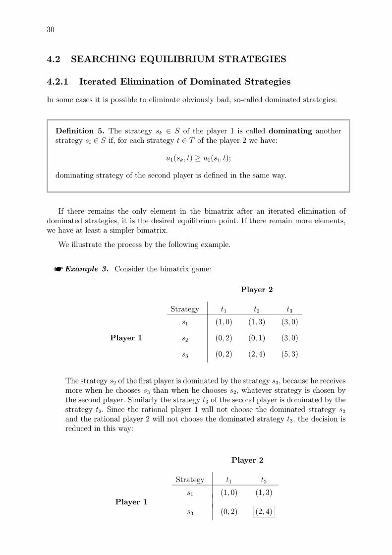
☛ Example 3. Consider the bimatrix game:
Player 2
Strategy t1 t2 t3
s1 (1, 0) (1, 3) (3, 0)
Player 1 s2 (0, 2) (0, 1) (3, 0)
s3 (0, 2) (2, 4) (5, 3)
The strategy s2 of the first player is dominated by the strategy s3, because he receivesmore when he chooses s3 than when he chooses s2, whatever strategy is chosen bythe second player. Similarly the strategy t3 of the second player is dominated by thestrategy t2. Since the rational player 1 will not choose the dominated strategy s2and the rational player 2 will not choose the dominated strategy t3, the decision isreduced in this way:
Player 2
Strategy t1 t2
s1 (1, 0) (1, 3)Player 1
s3 (0, 2) (2, 4)
4.2. SEARCHING EQUILIBRIUM STRATEGIES 31
Strategy t1 is dominated by the strategy t2, the second player therefore choosest2. The first player now decides between the values in the second column of thebimatrix, and since 1 < 2, he chooses s3. Hence an equilibrium point of the gameis (s3, t2) – think over the fact that in the original matrix, one-sided deviation fromthe equilibrium strategy do not bring an improvement to the ”deviant”.
☛ Example 4. An investor wants to build two hotels. One of them will be called Big(abbreviated as B); gaining the order for it will bring the profit of 15 million to thebuilding firm. The second hotel will be called Small (abbreviated as S); gaining theorder for it will bring the profit of 9 million to the building firm.There are two firms competing for the orders, we will denote them 1 and 2. Noneof them has a potential to build both hotels in full. Each firm can offer the buildingof one hotel or the cooperation on both of them. The investor has to realize thebuilding by force of these firms and he decides on the base of a sealed-bid method.The rules for splitting the orders according to offers are the following:
1. If only one firm bids for a contract on a hotel, it receives it all.
2. If two firms bid for a contract on the same hotel and none of them bids for thesecond one, the investor offers the cooperation to both firms on both hotels,the profits are split fifty-fifty.
3. If one firm bids for a contract on the whole building of a hotel and the secondfirm offers a collaboration, than the firm that bids the whole building receives60% and the second 40% in the case of B, and 80% versus 20% in the caseof S. On the building of the other hotel the firms will collaborate fifty-fifty(including splitting the profit).
In every case the total profit of 15 + 9 = 24 milion is split between the firms. Findoptimal strategies for both firms.
The payoffs corresponding to particular strategies can be represented by a bimatrix:
Firm 2
Strategy Big Small Cooperation
Big (12, 12) (15, 9) (13, 5; 10, 5)
Firm 1 Small (9, 15) (12, 12) (14, 7; 9, 3)
Cooperation (10, 5; 13, 5) (9, 3; 14, 7) (12, 12)
Strategy ”cooperation” is dominated by the strategy ”big” for both firms, we cantherefore elliminate the third row and the third column. Now we have a bimatrix withonly two rows and two columns (strategies ”big” and ”small”). Here the strategy ”small”is dominated by the strategy ”big” and can therefore be elliminated, too. There remainsthe only point: the strategy pair (”big”,”big”) and it is an equilibrium point.
32 4. BIMATRIX GAMES
4.2.2 Best Reply Correspondence
According to the definition, equilibrium strategies s∗, t∗ forming the equilibrium point(s∗, t∗) are mutually best replies in the sense that if the first player chooses his equilibriumstrategy s∗, then the second player can not improve his outcome by deviating from t∗,similarly the first player can not improve his outcome by deviating from s∗, provided thesecond player chooses t∗.
More exactly:
Definition 6. Best reply of player 1 to the strategy t of player 2 is definedas the set
R1(t) = {s∗ ∈ S; u1(s∗, t) ≥ u1(s, t) for each s ∈ S} . (4.3)
Similarly best reply of player 2 to the strategy s of player 1 is defined as theset
R2(s) = {t∗ ∈ T ; u2(s, t∗) ≥ u2(s, t) for each t ∈ T} . (4.4)
If the strategy sets consist of two elements for both players, the sets R1 and R2 arecurves in the plain – so-called reaction curves.
Theorem 2. (s∗, t∗) is an equilibrium point if and only if it is
s∗ = R1(t∗) and t∗ = R2(s
∗).
Proof. According to the definition, s∗ = R1(t∗) if and only if for each s ∈ S it is
u1(s∗, t∗) ≥ u1(s, t
∗), (4.5)
similarly t∗ = R2(s∗) if and only if for each t ∈ T it is:
u2(s∗, t∗) ≥ u1(s
∗, t). (4.6)
Inequalities (4.5), (4.6) correspond to the conditions for an equilibrium point given inDefinition 2.
Searching an equilibrium point, we can construct reaction curves and find theirintersection.
4.2. SEARCHING EQUILIBRIUM STRATEGIES 33
☛ Example 5. For the game from the example 1, the best reply of player 1 to thestrategy t1 of player 2 is the strategy s1, i.e.
R1(t1) = s1,
similarly the best reply of player 1 to the strategy t2 is the strategy s2, i.e.
R1(t2) = s2.
Similarly for the best replies of player 2:
R2(s1) = t1, R2(s2) = t1.
In this case, it is easy to find the pair of strategies that are mutually best replies: itis the pair (s1, t1) which is, according to the above discussion, an equilibrium pointof the game.
☛ Example 6. For the game from the example 2 we have
R1(t1) = s1, R1(t2) = s2.
R2(s1) = t2, R2(s2) = t1.
In this case, no pair of strategies consists from mutually best replies. As it wasalready mentioned, it is necessary to consider mixed strategies.
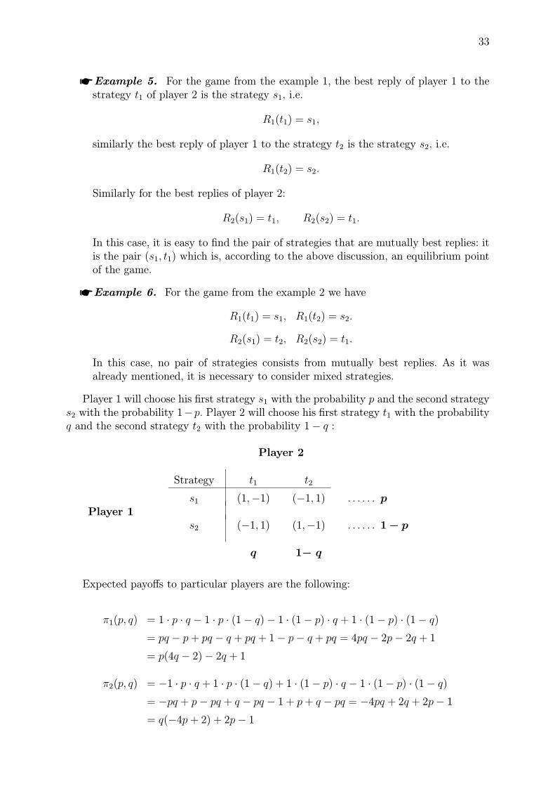
Player 1 will choose his first strategy s1 with the probability p and the second strategys2 with the probability 1−p. Player 2 will choose his first strategy t1 with the probabilityq and the second strategy t2 with the probability 1− q :
Player 2
Strategy t1 t2
s1 (1,−1) (−1, 1) . . . . . . p
Player 1s2 (−1, 1) (1,−1) . . . . . . 1− p
q 1− q
Expected payoffs to particular players are the following:
Now we will search best replies of the player 1 to various choices of probability q :
If 0 ≤ q < 12, then for a fixed value of q, π1(p, q) is a linear function with the negative
slope, which is therefore decreasing. Maximum of this function occurs for the leastpossible value of p, i.e. for p = 0; in this case it is: R1(q) = 0.
If q = 12, then π1(p,
12) = 0 is a constant function for which each value is maximal
and minimal – player 1 is therefore indifferent between both strategies, R1(12) = 〈0, 1〉.
If 12
< q ≤ 1, then for a fixed value of q, π1(p, q) is a linear function with the positive
slope, which is therefore increasing. Maximum occurs for the greatest possible value ofp, i.e. for p = 1; in this case it is R1(q) = 1.
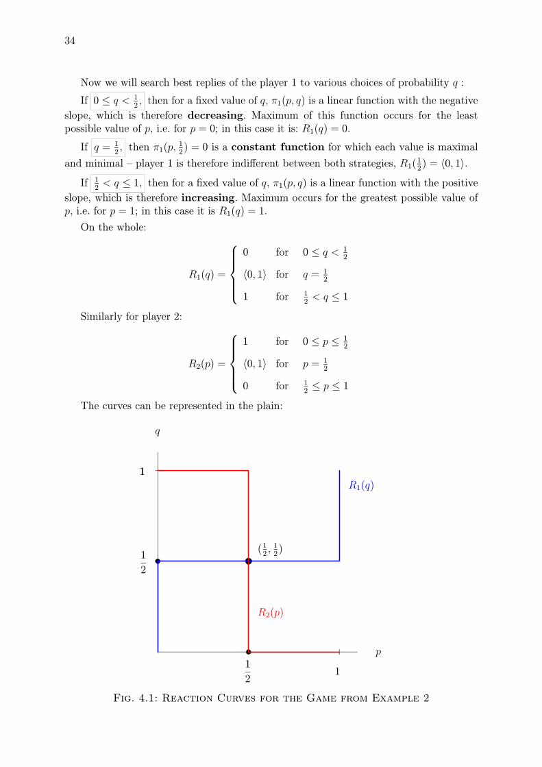
On the whole:
R1(q) =
0 for 0 ≤ q < 12
〈0, 1〉 for q = 12
1 for 12
< q ≤ 1
Similarly for player 2:
R2(p) =
1 for 0 ≤ p ≤ 12
〈0, 1〉 for p = 12
0 for 12≤ p ≤ 1
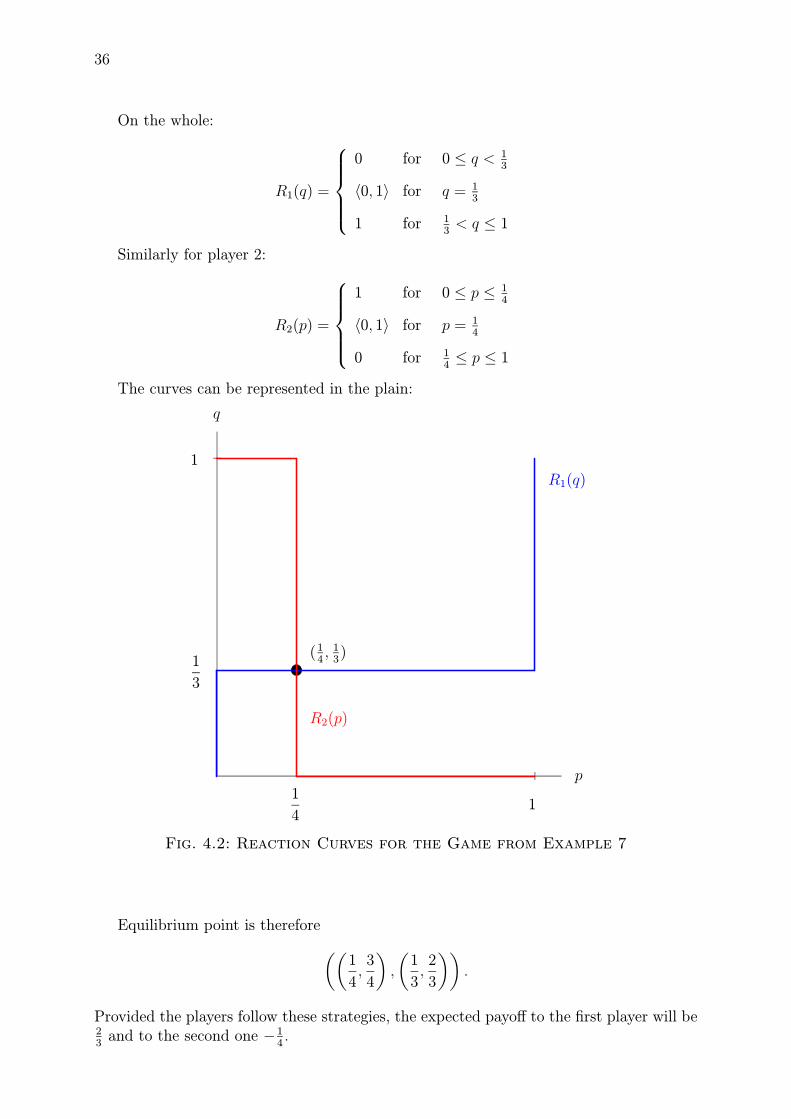
The curves can be represented in the plain:
p
q
1
21
1
2
1R1(q)
R2(p)
(12, 12)
1
Fig. 4.1: Reaction Curves for the Game from Example 2
4.2. SEARCHING EQUILIBRIUM STRATEGIES 35
Equilibrium point is therefore((1
2,1
2
)
,
(1
2,1
2
))
.
Provided the players follow these strategies, the expected payoff is 0 for each of them.
A Usefull Principle for Equilibrium Strategies Search:
A mixed strategy s∗ = (p1, . . . , pm) is the best reply to t∗ if and only if each of purestrategies that occur in s∗ with positive probability is the best reply to t∗.
The player who optimalizes using a mixed strategy is therefore indifferent amongall pure strategies that occur in a given mixed strategy with positive probabilities.
(Notice that if for example a pure strategy s1 would be more advantageous in a givensituation than s2, than whenever the player would be about to use s2, it would be betterto use s1 – we would not have an equilibrium point.)
☛ Example 7. Consider a bimatrix game
Player 2
Strategy t1 t2
s1 (4,−4) (−1,−1)Player 1
s2 (0, 1) (1, 0)
Expected values for particular players are the following:
π1(p, q) = 4pq − p(1− q) + 0 + (1− p)(1− q)
= p(6q − 2)− q + 1
π2(p, q) = −4pq − p(1− q) + (1− p)q + 0
= q(−4p+ 1)− p
Now we will search best replies of the player 1 to various choices of probability q :
If 0 ≤ q < 13, then for a fixed value of q, π1(p, q) is a linear function with the negative
slope, which is therefore decreasing. Maximum of this function occurs for the leastpossible value of p, i.e. for p = 0; in this case it is: R1(q) = 0.
If q = 13, then π1(p,
13) = 2
3is a constant function for which each value is maximal
and minimal – player 1 is therefore indifferent between both strategies, R1(13) = 〈0, 1〉.
If 13
< q ≤ 1, then for a fixed value of q, π1(p, q) is a linear function with the positive
slope, which is therefore increasing. Maximum occurs for the greatest possible value ofp, i.e. for p = 1; in this case it is R1(q) = 1.
36 4. BIMATRIX GAMES
On the whole:
R1(q) =
0 for 0 ≤ q < 13
〈0, 1〉 for q = 13
1 for 13
< q ≤ 1
Similarly for player 2:
R2(p) =
1 for 0 ≤ p ≤ 14
〈0, 1〉 for p = 14
0 for 14≤ p ≤ 1
The curves can be represented in the plain:
p
q
1
41
1
3
1R1(q)
R2(p)
(14, 13)
Fig. 4.2: Reaction Curves for the Game from Example 7
Equilibrium point is therefore
((1
4,3
4
)
,
(1
3,2
3
))
.
Provided the players follow these strategies, the expected payoff to the first player will be23and to the second one −1
4.
4.2. SEARCHING EQUILIBRIUM STRATEGIES 37
On the base of the above principle, searching an equilibrium point can be significantlysimplified:
If q is an equilibrium strategy of player 2, player 1 has to be indifferent between hispure strategies s1, s2 (compare Fig. 4.3). Hence the expected payoffs have to be the samefor both pure strategies of player 1 for the mixed strategy (q, 1− q) of player 2:
π1(1, q) = 4q − (1− q) = 0 + (1− q) = π1(0, q)
6q = 2 ⇒ q =1
3
Similarly, in order p is an equilibrium strategy of player 1, player 2 has to be indifferentbetween his pure strategies t1, t2 (compare Fig. 4.3). Hence the expected payoffs have tobe the same for both pure strategies of player 2 for the mixed strategy (p, 1− p) of player1:
π2(p, 1) = −4p+ (1− p) = −p+ 0 = π2(p, 0)
1 = 4p ⇒ p =1
4
In this way we have come to the same equilibrium point:((14, 34
),(13, 23
)).
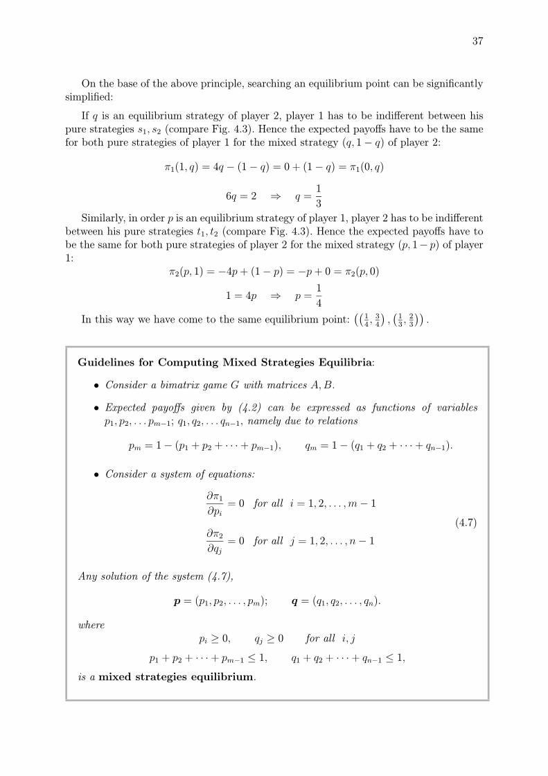
Guidelines for Computing Mixed Strategies Equilibria:
• Consider a bimatrix game G with matrices A,B.
• Expected payoffs given by (4.2) can be expressed as functions of variablesp1, p2, . . . pm−1; q1, q2, . . . qn−1, namely due to relations
So far we have met examples where only one equilibrium point existed, whatever in pureor mixed strategies. But often more equilibrium points exist and a question arises, whichof them shall be considered as optimal.
Let us start with several definitions.
Definition 7. Let (p, q) be an equilibrium point of the bimatrix game G such that
π1(p, q) ≥ π1(r, s) and π2(p, q) ≥ π2(r, s)
for any equilibrium point (r, s) of the game G. Then (p, q) is called dominatingequilibrium point of the game G.
If there exists the only equilibrium point, it is obviously dominating.
4.2. SEARCHING EQUILIBRIUM STRATEGIES 39
☛ Example 9. Consider a bimatrix game
((3, 2) (−1, 1)
(−2, 0) (6,5)
)
There exist two equilibrium points in pure strategies, namely (s1, t1) and (s2, t2).The second of them dominates the first one, since for the payoffs we have: 6 > 3a 5 > 2. Hence for both players it is the most advantageous to choose the secondstrategy.
☛ Example 10. Consider a bimatrix game
Player 2
t1 t2 t3
s1 (-2,-2) (-1,0) (8,6)
Player 1 s2 (0,-1) (5,5) (0,0)
s3 (8,6) (0,-1) (-2,-2)
In this game there exist three pure equilibrium points: (s1, t3), (s2, t2), (s3, t1). Thefirst and last ones are dominating. Nevertheless, since the players have no chanceto make a deal, it can happen that they choose strategy pairs (s1, t1) or (s3, t3) andreach the worst possible outcomes.
Definition 8. Let (p(j), q(j)), j ∈ J, are equilibrium points of a bimatrix game G.These points are called interchangeable, if the value of payoff functions π1(p, q) andπ2(p, q) do not change when we put any p
(j), j ∈ J instead of p and any q(j), j ∈ J
instead of q.
☛ Example 11. Let us change the bimatrix from the previous example:
Player 2
t1 t2 t3
s1 (8,6) (-1,0) (8,6)
Player 1 s2 (0,-1) (5,5) (0,0)
s3 (8,6) (0,-1) (8,6)
All dominating equilibrium points (s1, t1), (s1, t3), (s3, t1) and (s3, t3) are now in-terchangeable and the trouble from the previous example can not occur. This factmotivates the following definition.
40 4. BIMATRIX GAMES
Definition 9. All interchangeable dominating equilibrium points of a given game Gare called optimal points of the game G. If there exist such points in a game, thegame is called solvable.
☛ Example 12 – Battle of the Buddies.
Consider a married couple in which the partners have a bit different opinions ofhow to spend a free evening: the wife prefers the visit of a box match, the husbandprefers the visit of a football match. Payoffs are represented by the bimatrix
Husband
Box Football
Box (2, 1) (0, 0)Wife
Football (0, 0) (1, 2)
The game has two equilibrium points in pure strategies, namely
(box, box), (football, football),
and another equilibrium point in mixed strategies,((13, 23), (2
3, 13)), with the corresponding
values of expected payoffs(23, 23
).
p
q
11
3
2
3
1
R1(q)
R2(p)
Fig. 4.3: Reaction Curves for the Battle of the Buddies
These values can easily be found by solving the equation:
Since no equilibrium point is dominated, this game is not solvable in the sense of thedefinition 9.
4.3. EQUILIBRIUM STRATEGIES IN BIOLOGY 41
4.3 EQUILIBRIUM STRATEGIES IN BIOLOGY
4.3.1 Introduction
In biology, game theory is the main tool for the investigation of conflict and cooperation ofanimals and plants. As for zoological applications, the theory of games is used for the ana-lysis, modeling and understanding the fight, cooperation and communication of animals,coexistence of alternative traits, mating systems, conflict between the sexes, offspringsex ratio, distribution of individuals in their habitats, etc. Among botanical applicationswe can find the questions of seed dispersal, seed germination, root competition, nectarproduction, flower size, sex allocation, etc.
Apparently the first work where a game-theoretical approach was used (although theauthor was not aware of it), was Fisher’s book [6] from 1930; it came about in the con-nection with the evolution of the sex ratio and with the sexual selection. The first explicitand conscious application of game theory in biology is contained in Lewontin’s paper onevolution [9] from 1961. Nevertheless, Lewontin considered species to play a game againstthe nature, while the modern theory pictures members of a population as playing gamesagainst each other and studies the population dynamics and equilibria which can arise;this second approach was foreshadowed in the mentioned Fisher’s book [6] and developed– including explicit terminology of game theory – by W. D. Hamilton [7], [8], R. L. Trivers[13] and some others. However, these works remained isolated and they did not stir upany wider interest.A historical milestone is represented by the short but ”epoch-making” paper The Logic
of Animal Conflict by J. Maynard Smith and G. R. Price. This treatise, published in 1973,stimulated a great deal of successful works and applications of game theory in evolutionarybiology; the development of the following decade was summarized in Maynard Smith’sbook Evolution and the Theory of Games [11]. Not only proved game theory to providethe most satisfying explanation of the theory of evolution and the principles of behaviorof animals and plants in mutual interactions, it was just this field which turned out toprovide the most promising applications of the theory of games at all. Is this a paradox?How is it possible that the behavior of animals or plants prescribed on the base of game-theoretical models agree with the action observed in the nature? Can a fly or a fig tree,for example, be a rational decision-maker who evaluates all possible outcomes and by thetools of game theory selects his optimal strategy? How is it possible that even the lessdeveloped the thinking ability of an organism is, the better game theory tends to work?
As the birth of game theory von Neumann’s paper [?] from 1928 is usually considered; nevertheless,the origin of the theory as a ”real” mathematical discipline is connected with the book [12] of John vonNeumann and Oscar Morgenstern, first published in 1944; only then game theory became widely known.
42 4. BIMATRIX GAMES
4.3.2 The Game of Genes
The explanation is simple: the players of the game are not taken to be the organismsunder study, but the genes in which the instinctive behavior of these organisms is coded.The strategy is then the behavioral phenotype, i.e. the behavior preprogrammed by thegenes – the specification of what an individual will do in any situation in which it may finditself; the payoff function is a reproductive fitness, i.e. the measure of the ability of a geneto survive and spread in the genotype of the population in question. The main solutionconcept of this model the evolutionary stable strategy which is defined as a strategy suchthat, if all the members of a population adopt it, no mutant strategy can invade. In certainspecific situations, this somewhat vague concept is expressed more precisely. For example,the pairwise contests in an infinite asexual population can be modelled by a two-playernormal form game and the evolutionary stable strategy I is a strategy satisfying thefollowing conditions:
for all J 6= I either u1(I, I) > u1(J, I)
or u1(I, I) = u1(J, I) and u1(I, J) > u1(J, J);(4.8)
in biological terms, the value of the payoff function u1(s1, s2) is the expected change offitness of an individual adopting a strategy s1 against an opponent adopting s2 (fitnesscan be measured for example by the number of offspring).
In short, to understand the basic principles of so-called ”genocentric” conception of theevolution, it suffices to imagine that about four thousand million years ago a remarkablemolecule was formed by accident that was able to create copies of itself – we will call itthe replicator. It started to spread its copies; during the replication sometimes a mistakeor mutation occurred, some of these mutations led to replicators that were more successfulin mutual contests and in reproduction. Some of them could discover how to break upmolecules of rival varieties chemically, others started to construct for themselves contai-ners, vehicles for their continued existence. Such replicators survived, that had better andmore effective ”survival machines”. Generation after generation, the survival machines ofgenes, i.e. the organisms controlled by the genes, compete in mutual contests; the genesthat choose the best strategy for their machine spread themselves and step by step theirlearning proceeds. The result is that these machines act in the same way as game theorywould calculate – instead of the calculation they have come to the equilibrium strategiesby gradual adaptation and natural selection.
[11], p. 204.Due to the symmetry, the pair of strategies (I, I) form an equilibrium point.It shall be noted that there exist good field measurements of costs and benefits in nature, which have
been plugged into particular models; see e.g. [3]. Hence the payoff can really be measured quantitatively.
4.3. EQUILIBRIUM STRATEGIES IN BIOLOGY 43
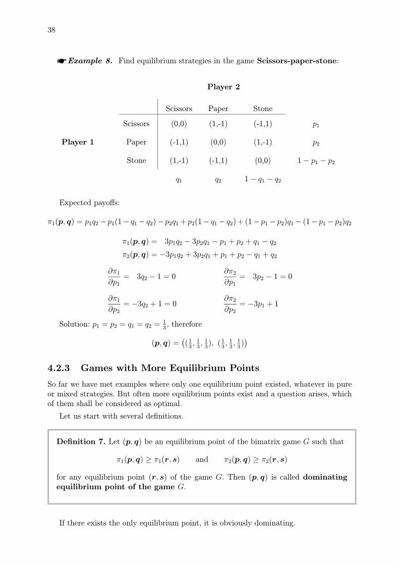
Equilibrium Strategies and Learning
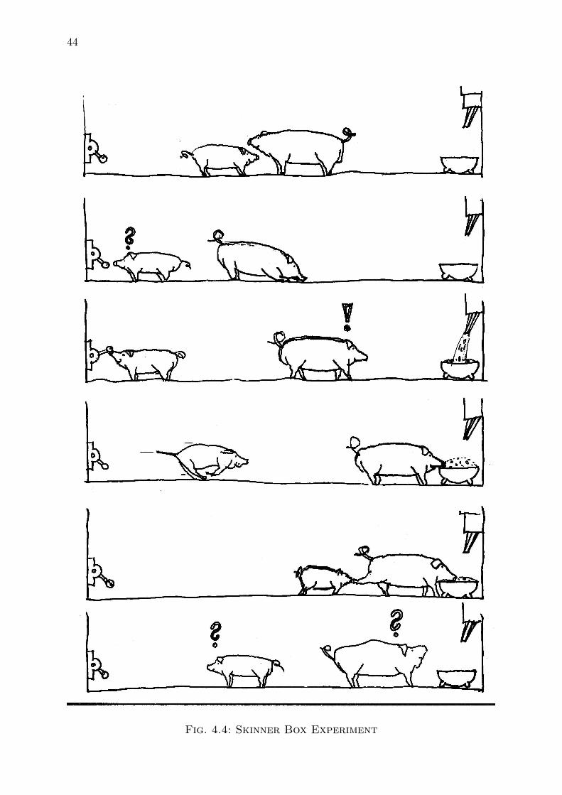
An illustrative analogy of the slow evolution process is the learning of an individual whofinds himself repeatedly in the same conflict situation during his relatively short lifetime.Apparently the most interesting experiment was made in 1979 by B. A. Baldwin andG. B. Meese with the Skinner sty: there is the snout-lever at one end of the sty, the fooddispenser at the other. Pressing the lever causes pureing the food down a chute. Baldwinand Meese placed two domestic pigs into this sty. Such couple always settles down intoa stable dominant/subordinate hierarchy. Which pig will press the lever and run acrossthe sty and which one will be sitting by the food trough? The situation is schematicallyillustrated in Fig. 1.The strategy ”If dominant, sit by the food trough; if subordinate, work the lever”
sounds sensible, but would not be stable. The subordinate pig would soon give up pressingthe lever, for the habit would never be rewarded. The reverse strategy ”If dominant, workthe lever; if subordinate, sit by the food trough” would be stable – even though if it hasthe paradoxical result that the subordinate pig gets most of the dominant pig when hecharges up from the other end of the sty. As soon as he arrives, he has no difficulty intossing the subordinate pig out of the trough. As long as there is a crumb left to rewardhim, his habit of working the lever will persist.
Using the theory of games, we would model the situation by a bimatrix game:
Press the lever Sit by the trough
Press the lever (8,−2) → (6,4)
↑Sit by the trough (10,−2) → (0, 0)
Rational players would come to the equilibrium strategies in the following way. Forthe second player – the subordinate pig – the first strategy is dominated by the secondone and can be therefore eliminated. The first player – the dominant pig – presumes therationality of his opponent and hence decides between the profit of 0 or 6 units in thesecond column, which leads him to the choice of the first strategy. Indeed, the couple ofstrategies (press the lever, sit by the trough) is an equilibrium point.
For more details see [4], pp. 286–287, and the original paper [2] by Baldwin and Meese.We consider the profit from the whole ration to the extent of 10 utility units, the loss caused by
the labor connected with pressing the lever and running −2 units and the amount of food which thesubordinate pig manages to eat before he is tossed out by the dominant one, 4 units (these units werechosen at random – from the strategic point of view nothings changes when the labor is evaluated withan arbitrary negative number, the waiting subordinate pig receives nonnegative number of units andnonnegative number of units remains for the dominant one.
44 4. BIMATRIX GAMES
Fig. 4.4: Skinner Box Experiment
4.3. EQUILIBRIUM STRATEGIES IN BIOLOGY 45
46 4. BIMATRIX GAMES
4.3.3 Conclusion
There are many interesting examples in the domain of biology which can be used notonly to motivate the students or liven up the lessons, but also to show how evolutionreally works – and getting to the heart of the evolution principles and hence to the heartof our lives is an exceptionally exciting experience. We ask the kind reader to take thiscontribution as the invitation to the reading of the books [4] and [5] by R. Dawkins, thebook [11] by Maynard Smith – the cited literature can be a good beginning of a morein-depth study.
Several remarks should be added in conclusion. First, the modern theory of evolutionbased on ”games of selfish genes” is much more satisfactory than the former theory whichconsidered the organisms acting ”for the good of the species”. In addition to all itemssolved by the ”group selection theory” (e.g. the existence of ”limited war” strategies andaltruism among non-relatives), the genocentric one can explain most of contradictions andquestions that the former theory can not answer.What is mainly surprising but auspicious, is the fact that the gene’s-eye view of evo-
lution provides the solid explanation of the existence of a real altruism in the nature: notonly among relatives, but also among non-relative individuals who interact in a long run –many instinctively acting species shall be taken as shining examples by us humans, oftengoverned by negative emotions. For example, a functioning reciprocal altruism underliesthe regular alternation of the sex roles in the hermafrodite sea bass, the reciprocal helpbetween mails of pavian anubi to fight off an attacker during the time one of them is ma-ting, or the blood-sharing by the great mythmakers vampires (the bats eating the cattleblood). In the words of R. Dawkins, . . . vampires could form the vanguard of a comfortablenew myth, a myth of sharing, mutualistic cooperation. They could herald the benignantidea that, even with selfish genes at the helm, nice guys can finish first.
[4], p. 233.
4.4. REPEATED GAMES – PRISONER’S DILEMMA 47
4.4 REPEATED GAMES – PRISONER’S DILEMMA
4.4.1 Examples
☛ Example 13 – Prisoner’s Dilemma 1
One of the interpretations of the conflict that is called Prisoner’s dilemma is thefollowing one:
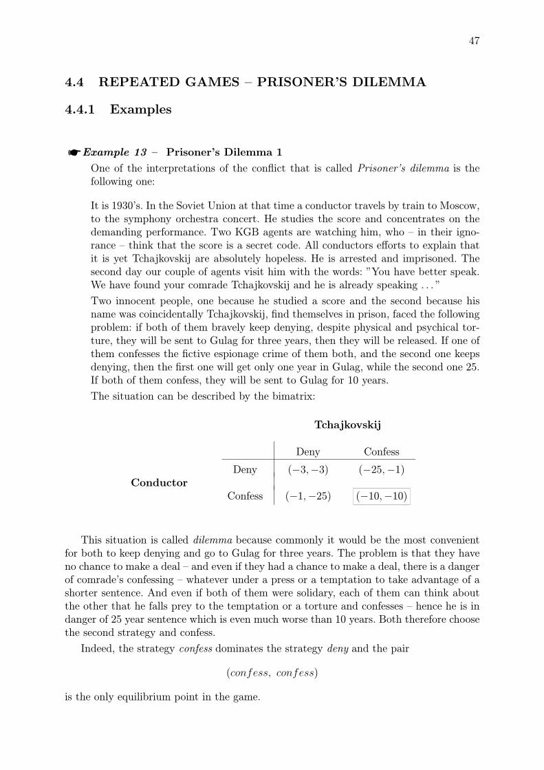
It is 1930’s. In the Soviet Union at that time a conductor travels by train to Moscow,to the symphony orchestra concert. He studies the score and concentrates on thedemanding performance. Two KGB agents are watching him, who – in their igno-rance – think that the score is a secret code. All conductors efforts to explain thatit is yet Tchajkovskij are absolutely hopeless. He is arrested and imprisoned. Thesecond day our couple of agents visit him with the words: ”You have better speak.We have found your comrade Tchajkovskij and he is already speaking . . . ”
Two innocent people, one because he studied a score and the second because hisname was coincidentally Tchajkovskij, find themselves in prison, faced the followingproblem: if both of them bravely keep denying, despite physical and psychical tor-ture, they will be sent to Gulag for three years, then they will be released. If one ofthem confesses the fictive espionage crime of them both, and the second one keepsdenying, then the first one will get only one year in Gulag, while the second one 25.If both of them confess, they will be sent to Gulag for 10 years.
The situation can be described by the bimatrix:
Tchajkovskij
Deny Confess
Deny (−3,−3) (−25,−1)Conductor
Confess (−1,−25) (−10,−10)
This situation is called dilemma because commonly it would be the most convenientfor both to keep denying and go to Gulag for three years. The problem is that they haveno chance to make a deal – and even if they had a chance to make a deal, there is a dangerof comrade’s confessing – whatever under a press or a temptation to take advantage of ashorter sentence. And even if both of them were solidary, each of them can think aboutthe other that he falls prey to the temptation or a torture and confesses – hence he is indanger of 25 year sentence which is even much worse than 10 years. Both therefore choosethe second strategy and confess.
Indeed, the strategy confess dominates the strategy deny and the pair
(confess, confess)
is the only equilibrium point in the game.
48 4. BIMATRIX GAMES
☛ Example 14 – Prisoner’s Dilemma 2
More generally, prisoner’s dilemma is a name for every situation of the type (comparethe example 13):
Cooperation can express whatever – the strategy pair (cooperate, cooperate) corre-sponds to mutually solidary action.
Where Prisoner’s Dilemma Occurs – Some More Examples
• Building the Sewage Water Treatment Plant (two big hotels by one mountainlake):
– Cooperate = build the purify facility
– Defect = do not build it
– Reward = pure water attracts tourists – customers, profits increase, neverthe-less, we had to invest a certain sum of money
– Temptation = take advantage of the purify facility of the second hotel and saveon the investment
– Punishment = polluted water discourages tourists, the profit decreases to zero
• Duopolists:
– Cooperate = collude on the optimal total production (corresponding to mono-poly)
– Defect = break the deal
– Reward = the highest total profit
– Temptation = produce somewhat more at the expense of the second duopolist
– Punishment = less profit for both
4.4. REPEATED GAMES – PRISONER’S DILEMMA 49
• Removing the Parasites:
– Cooperate = mutual removing of parasites
– Defect = have removing done by the comrade but do not return the favor
– Reward = I will be free of parasites, nevertheless I will pay it by removingyours
– Temptation = I will be free of parasites without paying it back
– Punishment = all are full of parasites which is much worse than a slight effortto remove the other’s parasites
• Public Transportation:
– Cooperate = pay the fare
– Defect = do not pay
– Reward = public transportation runs, I can use it, nevertheless I have to paya certain sum every month.
– Temptation = use the public transportation but do not pay
– Punishment = (almost) nobody pays, the public transportation is dissolved, Ihave to pay a taxi which is much more expensive than the original fare payment
• Television Licence Fee:
– Cooperate = pay
– Defect = do not pay
– Reward = public service broadcast works, I can watch it, but I have to paysome small sum of money
– Temptation = do not pay and watch
– Punishment = (almost) nobody pays, the broadcast is dissolved
• Battle:
– Cooperate = fight
– Defect = hide
– Reward = victory but also a risk of injury
– Temptation = victory without a risk of injury
– Punishment = the enemy wins without any fighting
• Nuclear Armament:
– Cooperate = disarm
– Defect = arm
– Reward = the world without nuclear threat
– Temptation = to be the only one armed
– Punishment = all arm, pay much money for it, moreover a danger threats
50 4. BIMATRIX GAMES
4.4.2 Repeated Prisoner’s Dilemma
In the case of infinite or indeterminate time horizon, Cooperate is not necessarily irrational:
☛ Example 15 – Prisoner’s Dilemma 3
Consider the following variant of Prisoner’s dilemma:
Player 2
Cooperate Defect
Cooperate (3, 3) (0, 5)Player 1
Defect (5, 0) (1, 1)
Imagine that the game will be repeated with the probability of 2/3 in each round thatthe next round occurs, too.
When both players cooperate, the expected payoff for each of them is:
πC = 3 + 3 ·23+ 3 · (2
3)2 + 3 · (2
3)3 + · · ·+ 3 · (2
3)n + · · ·
Strategy in repeated game is a complete plan how the player will act in the wholecourse of the game in all possible situations in which he can find himself.
For example, consider a strategy Grudger:
Cooperates until the second has defected, after that move defects forever.
When two Grudgers meet in a game, they will cooperate all the time and each of themreceives the value πG = πC .It can easily be proven that the pair of strategies
(Grudger, Grudger)
is an equilibrium point of the game in question.
Consider a Deviant who deviates from the Grudger strategy played with Grudger.In some round this Deviant defects, although the Grudger has cooperated (this can alsohappen in the first round). Let this deviation occurs first in the round n + 1. Since theDeviant plays with the Grudger, in the next round the opponent chooses his strategydefect and holds on it forever. The Deviant can not therefore obtain more than
πD = 3 + 3 ·23+ 3 · (2
3)2 + 3 · (2
3)3 + · · ·+ 3 · (2
3)n−1 + 5 · (2
3)n + 1 · (2
3)n+1 + · · ·
Since
πG − πD = (3− 5) · (23)n + (3− 1) · (2
3)n+1 + · · ·+ (3− 1) · (2
3)n+k + · · ·
= −2 · (23)n + 2 · (2
3)n+1 + · · ·+ 2 · (2
3)n+k + · · ·
= (23)n
(
−2 + 2 · 23·1
1− 23
)
= (23)n · 2 > 0,
4.4. REPEATED GAMES – PRISONER’S DILEMMA 51
it does not pay to deviate.
Similarly, we can consider the strategy Tit for Tat, which begins with cooperationand then plays what its opponent played in the last move. The pair
(Tit for Tat, Tit for Tat)
is an equilibrium point, too.
Examples of Strategies in Repeated Prisoner’s Dilemma
Always Cooperates
Always Defects
Grudger, Spiteful: Cooperates until the second has defected, after that move defectsforever (he does not forgive).
Tit for Tat: begins with cooperation and then plays what its opponent played in thelast move (if the opponent defects in some round, Tit for Tat will defect in thefollowing one; to cooperation it responds with cooperation).
Mistrust Tit for Tat: In the first round it defects, than it plays opponent’s move.
Naive Prober: Like Tit for Tat, but sometimes, after the opponent has cooperated, itdefects (e.g. at random, in one of ten rounds in average).
Remorseful Prober: Like Naive Prober, but he makes an effort to end cycles C–Dcaused by his own double-cross: after opponent’s defection that was a reaction tohis unfair defection, he cooperates for one time.
Hard Tit for Tat: Cooperates unless the opponent has defected at least once in thelast two rounds.
Gradual Tit for Tat: Cooperates until the opponent has defected. Then, after thefirst opponent’s defection it defects once and twice it cooperates, after the seconddefection it defects in two subsequent rounds and twice it cooperates, . . . , after then-th opponent’s defection it defects in n subsequent rounds and twice it cooperates,etc.
Gradual Killer: In the first five rounds it defects, than it cooperates in two rounds. Ifthe opponent has defected in rounds 6 and 7, than the Gradual Killer keeps defectingforever, otherwise he keeps cooperation forever.
Hard Tit for 2 Tats: Cooperates except the case when the opponent has defected atleast in two subsequent rounds in the last three rounds.
Soft Tit for 2 Tats: Cooperates except the case when the opponent has defected inthe last two subsequent rounds.
Slow Tit for Tat: Plays C–C, then if opponent plays two consecutive times the samemove, plays its move.
52 4. BIMATRIX GAMES
Periodically DDC: Plays periodically: Defect–Defect–Cooperate
Periodically SSZ: Plays periodically: Cooperate–Cooperate–Defect
Soft Majority: Cooperates, than plays opponent’s majority move, if equal then coo-perates.
Hard Majority: Cooperates, than plays opponent’s majority move, if equal then de-fects.
Pavlov: Cooperates if and only if both players opted for the same choice in the previousmove, otherwise it defects.
Pavlov Pn: Adjusts the probability of cooperation in units of 1/n according to theprevious round: when it cooperated with the probability p in the last round, theprobability of cooperation in the next round is
p ⊕ 1n= min(p+ 1
n, 1) if it obtained R = reward ;
p ª 1n= max(0, p − 1
n) if it obtained P = punishment ;
p ⊕ 2nif it obtained T = temptation ;
ª 2nif it obtained S = sucker .
Random: Cooperates with the probability 1/2.
Hard Joss: Plays like Tit for Tat, but it cooperates only with the probability 0.9.
Soft Joss: Plays like Tit for Tat, but it defects only with the probability 0.9.
Generous Tit for Tat: Plays like Tit for Tat, but it after the defection it cooperateswith the probability
g(R,P, T, S) = min
(
1−T − R
R − S,R − P
T − P
)
.
Better and Better In n-th round it defects with the probability (1000 − n)/1000, i.e.the probability of defection is lesser and lesser.
Worse and Worse: In n-th round it defects with the probability n/1000, i.e. the pro-bability of defection is greater and greater.
4.4. REPEATED GAMES – PRISONER’S DILEMMA 53
Axelrod’s Tournament
In 1981 Robert Axelrod organized a computer tournament in which 15 different strategiesfor the repeated prisoner’s dilemma sent by prominent game theorists fought in pairwisematches, each math consisting of 200 rounds (totally 15×15 matches). The points obtainedon the base of the matrix from example 15 were summed.
To a great surprise of all involved, the highest score was won by the simple Tit forTat that was sent by Anatol Rapoport, psychologist and game theory specialist.
In his discussion of the tournament, Axelrod distinguished the following categories ofstrategies:
• Nice Strategy – never defects first (only in retaliation),
Nasty Strategy – at least sometimes it defects first.
There were eight nice strategies in the tournament and they took the first eightplaces (the most successful one obtained 504,5 points which corresponds to 84% ofthe standard of 600 points, other nice strategies obtained 83,4%–78,6%; the mostsuccessful of nasty strategies gained only 66,3%).
• Forgiving Strategy – can retaliate but it has a short memory, forgets the oldunfairness,
Non-Forgiving Strategy – never forgets old unfairness, never extricates froma cycle of mutual retaliations – not in the game with a remorseful opponent.
• Clear Strategy – it is only interested in its own profit, not in the defeat of theopponent,
Envious Strategy
• Retaliatory Strategy – does not let nasty strategies to exploit it,
Non-Retaliatory Strategy
The Second Tournament
In the second Axelrod tournament the number of rounds was not strictly given but thetournament went analogically with the evolution based on the natural selection: all stra-tegies gained a payoff corresponding to the number of offspring, the total number ofindividuals was keeping constant. More successful strategies reproduced at the expenseof less successful; after about 1000 generations the stability was reached. The winner wasagain Tit for Tat.
54 4. BIMATRIX GAMES
Occurrences of Repeated Prisoner’s Dilemma (further examples)
• Front Linie – Live and Let Live:
– Cooperate = live and let live
– Defect = kill every man from the opposite side when the opportunity knocks
– Reward = survival of long war years
– Temptation = take advantage of the situation that the opponent is an easychased and earn for example a medal – it is afterall better to remove theenemy
– Punishment = all are upon the guard all the time. . .
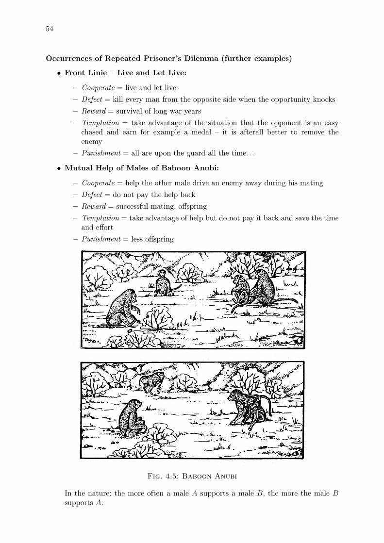
• Mutual Help of Males of Baboon Anubi:
– Cooperate = help the other male drive an enemy away during his mating
– Defect = do not pay the help back
– Reward = successful mating, offspring
– Temptation = take advantage of help but do not pay it back and save the timeand effort
– Punishment = less offspring
Fig. 4.5: Baboon Anubi
In the nature: the more often a male A supports a male B, the more the male Bsupports A.
4.4. REPEATED GAMES – PRISONER’S DILEMMA 55
• Fig Tree and Chalcidflies:
– Cooperate = balanced ratio of pollinated flowers and flowers with laied eggsinside the fig
– Defect = lay eggs to a greater number of flowers
– Reward = genes spread
– Temptation = lay eggs to a greater number of flowers and hence to encreasethe number of offspring
– Punishment = the fig hosting the treacherous Calcidfly family is thrown downand the whole family dies out
• Sexual Roles Alternating by Hermaphrodite Grouper:
– Cooperate = if I am a male now, I will became a female the next time
– Defect = became a male again after acting a male
– Reward = living together in harmony, many offspring
– Temptation = repeat an easy male role
– Punishment = the relation breaks down
• Desmodus Rotundus Vampire (a bat sucking mammal blood) – feedinghungry individuals:
– Cooperate = after a successful hunt, feed unsuccessful individuals ”colleagues”
– Defect = keep all blood
– Reward = long-run successful survival
– Temptation = in the case of need, let the colleagues to feed me, do not sharethe catch with the others
– Punishment = in the case of unsuccessful hunt, starving out
In the nature: the individuals that have returned from a unsuccessful hunt arefeeded by successful ones, even non-relatives; they recognize each other.
Fig. 4.6: Desmodus Rotundus Vampires
56 REFERENCES
References
[1] Axelrod, R.: The Evolution of Cooperation. Basic Books, New York, 1984.
[2] Baldwin, B. A.; Meese, G. B.: Social Behaviour in Pigs Studied by Means of OperantConditioning. Animal Behaivour, 27(1979), pp. 947–957.
[3] Brockmann, H. J.; Dawkins, R.; Grafen, A.: Evolutionarily Stable Nesting Strategyin a Digger Wasp. Journal of Theoretical Biology, 77(1979), pp. 473–496.
[4] Dawkins, R.: The Selfish Gene. Oxford University Press, Oxford, 1976 (Czechtranslation by V. Kopsý: Sobecký gen, Mladá Fronta, Praha, 2003).
[5] Dawkins, R.: The Blind Watchmaker. Harlow, Longman, 1986 (Czech translation byT. Grim: Slepý hodin ař, Paseka, Praha, 2002).
[6] Fisher, R. A.: The Genetical Theory of Natural Selection. Clar. Press, Oxford, 1930.
[7] Hamilton, W. D.: The Genetical Evolution of Social Behaviour I, II. Journal of The-oretical Biology 7(1964), pp. 1–16; 17–52.
[8] Hamilton, W. D.: Extraordinary Sex Ratios. Science 156(1967), pp. 477–488.
[9] Lewontin, R. C.: Evolution and the Theory of Games. Journal of Theoretical Biology1(1961), pp. 382–403.
[10] Maynard Smith, J. – Price, G. R.: The Logic of Animal Conflict. Nature 246(1973),pp. 15–18.
[11] Maynard Smith, J.: Evolution and the Theory of Games. Cambridge, CambridgeUniversity Press, 1982.
[12] von Neumann, J.; Morgenstern, O.: Theory of Games and Economic Behavior. Prin-ceton University Press, Princeton, 1944.
[13] Trivers, R. L.: The Evolution of Reciprocal Altruism. Quaterly Review of Biology46(1971), pp. 35–57.
[14] Williams, G. C.: Adaptation and Natural Selection. Princeton University Press, Prin-ceton, 1966.
[15] Williams, G. C.: Sex and Evolution. Princeton University Press, Princeton, 1975.
4.5. ANTAGONISTIC GAMES 57
4.5 ANTAGONISTIC GAMES
4.5.1 Two-Player Antagonistic Game
Definition 10. Two-player antagonistic game is a normal form game withconstant sum of payoffs:
(Q = {1, 2};S, T ;u1(s, t), u2(s, t))
u1(s, t) + u2(s, t) = const. for each (s, t) ∈ S × T.(4.9)
When the sum of payoffs in the game (4.9) is equal to zero, we simply write
u1(s, t) = u2(s, t) = u(s, t);
the normal form is:
(Q = {1, 2};S, T ;u(s, t)) (4.10)
For equilibrium strategies s∗, t∗ in a zero-sum game it is:
u(s, t∗) ≤ u(s∗, t∗) ≤ u(s∗, t) for all s ∈ S, t ∈ T. (4.11)
The value u(s∗, t∗) is called the value of the game.
It can be proven that to each two-player constant sum normal form game (4.9) azero sum normal form game can be assigned which is strategically equivalent to theoriginal game, i.e. every pair of strategies s, t, that is an equilibrium in the original gameis an equilibrium in the corresponding zero sum game, too, and vice versa. More exactly:
Theorem 3. Let (4.9) be a two-player constant sum game where the sum of payoffsequals K. Then s∗, t∗ are equilibrium strategies in the game (4.9) if and only if s∗, t∗
are equilibrium strategies in the zero sum game (4.10) where
u(s, t) = u1(s, t)− u2(s, t).
4.5.2 Matrix Games
Two-player zero-sum games with finite strategy sets
S = {s1, s2, . . . sm}, T = {t1, t2, . . . tn} (4.12)
whose elements express payoffs to the first player (payoffs to the second player have alwaysthe opposite value).
58 REFERENCES
Equilibrium Strategies in Matrix Games
When a so-called saddle point, i.e. an element that represents the minimum in therow and maximum in the column exists, then this element gives equilibrium strategiesand hence a value of the game, e.g.:
A =
5 4 4 5−4 5 3 97 8 −1 8
(4.14)
To find the saddle point, we can proceed in the following way: for each row we findthe minimum (such element represents the least guaranteed profit to the row player) andthen we find the maximal element of these minimas (for the corresponding row the leastguaranteed profit is the highest), so-called lower value of the game,
v = maxi=1,2,...,m
minj=1,2,...,n
aij . (4.15)
Similarly, for each column we find the maximum (such element represents the greatestguaranteed loss of the column player) and then we find the minimal element of thesemaximas (for the corresponding column the greatest guaranteed profit is the least), so-called upper value of the game,
v = minj=1,2,...,n
maxi=1,2,...,m
aij . (4.16)
In general, it isv ≤ v. (4.17)
Theorem 4. If, for a given matrix A it is v = v, than A has a saddle point.
The common value v = v = v is called the value of the game and the correspondingstrategies of the first and second player are called maximin and minimax strategies,respectively.
For the above matrix (4.14) we have
A =
5 4 4 5−4 5 3 97 8 −1 8
4−4−1
7 8 4 9
Unfortunately, the saddle point does not always exist, for example:
A =
(1 −1
−1 1
)
, v = −1, v = 1; B =
(0 −5/2 −2
−1 3 1
)
, v = −1, v = 0.
Hence, as before, it is necessary to introduce mixed strategies.
4.5. ANTAGONISTIC GAMES 59
Theorem 5. Fundamental Theorem on Matrix Games.In mixed strategies, every matrix game has at least one equilibrium point.
Again, the corresponding mixed strategies of the first and second player are calledmaximin and minimax strategies, respectively.
In other words, for every matrix A there exist vectors p∗ ∈ Ss, q∗ ∈ T s, such that:
pAq∗T ≤ p
∗Aq∗T ≤ p
∗AqT for all p ∈ Ss, q ∈ T s. (4.18)
Theorem 6. Equilibrium mixed strategies in a matrix game do not change when thesame (but arbitrarily chosen, positive or negative) number c is added to all elementsof the matrix. The value of the game with the matrix changed in this way, is v + cwhere v is the value of the original game.
4.5.3 Graphical Solution of 2× n Matrix Games
Expected values of player 1 for his mixed strategy (p, 1 − p) and second player’s purestrategies are:
For every p ∈ 〈0, 1〉 the value minj=1,2,...,n gj(p) gives the least guaranteed profit toplayer 1. Since the game is antagonistic, player 1 is looking for such value of p thatmaximizes this guaranteed profit:
p∗ := arg maxp∈〈0,1〉
minj=1,2,...,n
gj(p). (4.20)
First consider the functionϕ(p) := min
j=1,2,...,ngj(p). (4.21)
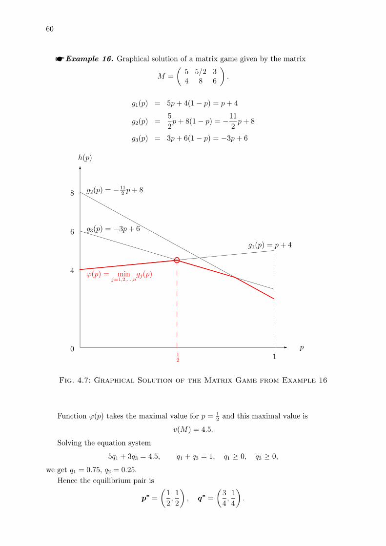
This function is concave and it consists of a finite number of line segments; it is thereforeeasy to find it maximum. The sought-after value of the game is then
v = ϕ(p∗) := maxp∈〈0,1〉
ϕ(p) (4.22)
and the sought-after mixed equilibrium strategy of player 1 is (p∗, 1− p∗).
If the extreme occurs in a point p∗ where gj(p∗) = gk(p
∗) = v for unique strategies j, kthen the components of a mixed equilibrium strategy of player 2 with indices differentfrom j, k are equal to zero. The components that can be non-zero can be obtained bysolving one of the equation systems
Suppose that all elements of the matrix A are positive (if not, it is possible to adda positive number, high enough – as we know, the new game would be strategicallyequivalent).
We will proceed analogously to searching pure equilibrium strategies.
For arbitrary but fixed p, the first player searches hisminimal guaranteed payoff h.
Considerh = min
∀j{a1jp1 + a2jp2 + · · ·+ amjpm} . (4.26)
Obviously, we have
h ≤ a1jp1 + a2jp2 + · · ·+ amjpm for all j ∈ {1, 2, . . . , n}. (4.27)
For any j the expression on the right gives the expected payoff to the first player when hechooses a mixed strategy p and the second player chooses a pure strategy tj . Expectedvalue of the payoff π(p, q) for the mixed strategy q of the second player is a linearcombination of these values with coefficients q1, q2, . . . , qn, that sum up to 1. We can easilyperceive that putting the mention linear combination on the right side of the inequality(4.27), remains unchanged:
The value h is therefore a minimal guaranteed payoff to the player 1, whichever pureor mixed strategy is chosen by the opponent (due to (4.26), h is the greatest numbersatisfying the last inequality).
62 REFERENCES
Let us divide the inequalities (4.27) by h
1 ≤ a1jp1h+ a2j
p2h+ · · ·+ amj
pm
h
and denote
yi =pi
h; obviously we have: y1 + y2 + · · ·+ ym =
1
h.
We come to the inequality
1 ≤ a1jy1 + a2jy2 + · · ·+ amjym . (4.28)
To maximize the minimal guaranteed payoff means to maximize h, i.e.
This is exactly the dual problem of linear programming (if h should be the valueof the game, it is necessary for both numbers to be the same).
4.6. GAMES AGAINST P-INTELLIGENT PLAYERS 63
4.6 GAMES AGAINST P-INTELLIGENT PLAYERS
4.6.1 Fundamental Concepts
Definition 11. A player behaving with probability p like a normatively intelligent pla-yer and with probability 1−p like a random mechanism will be called a p-intelligentplayer.
Parameter p characterizes the degree of deviation from the rational decision making.If p = 0, the player behaves in fact as a random mechanism, if p = 1, he is an intelligentplayer.
It is clear that it is not reasonable to apply the same strategies against the p-intelligentopponents as against intelligent opponents. Consider the case of matrix games.
Definition 12. The optimal strategy for the intelligent player is a row ofthe matrix A that maximizes the mean value of payoff when the p-intelligent playerapplies strategy
s(p) = py∗ + (1− p)r
where y∗ is a Nash equilibrium strategy of player 2 and r is a uniform probabilitydistribution over columns.
☛ Example 17. Investigate a matrix game defined by the matrix
3 3 3 37 1 7 73 1 −1 28 0 8 8
Solution
The unique pair of equilibrium strategies is
x∗ = (1, 0, 0, 0), y∗ = (0, 1, 0, 0).
If player 2 is p-intelligent, player 1 expects that player 2 is going to use the strategy
• the first row is an optimal strategy for player 1 if p ∈ 〈5/9, 1〉
• the second row is an optimal strategy for player 1 if p ∈ 〈1/3, 5/9〉
• the fourth row is an optimal strategy for player 1 if p ∈ 〈0, 1/3〉
• the third row is never an optimal strategy
64 REFERENCES
How much we may lose if we apply a strategy which is optimal against a fully intelligentplayer when we play against a partly intelligent player?
Definition 13. The function f(p), representing the average additional player’s 1 profitdue to his deviation from the equilibrium strategy x∗ is called excess function.
If player 1 uses the optimal strategy against the p-intelligent player, he receives thepayoff
maxi
a(i)s(p),
where a(i) means the i-th row of the matrix A and i goes over all rows of A, that is i =1, 2, . . . ,m. If he mechanically applies the strategy against the fully intelligent opponents,he receives
x∗T As(p).
Therefore,f(p) = max
i
[a(i)s(p)
]− x∗T As(p). (4.33)
☛ Example 18. For the game from example 17 we have
f(p) =
134− 214p for p ∈ 〈0, 1
3〉
114− 154p for p ∈ 〈1
3, 59〉
0 for p ∈ 〈59, 1〉
The following theorem confirms the fact that taking into account the decreased intel-ligence of the opponent is always an advantage.
Theorem 7. For any matrix game the excess function is a nonnegative, by partslinear, continuous and nonincreasing function on the interval 〈0, 1〉.
In other words, the difference between what we get when applying the strategy basedon the correct assessment of the opponent’s intelligence is always at least so great aswhen we simply apply the strategy optimal against normatively intelligent player. Thedifference decreases or remains the same when the intelligence of the opponent increases.


![NATIONAL INSTITUTE OF TECHNOLOGY DURGAPUR … · 2016-09-09 · Bimatrix games: LCP formulation, Lemke’s salgorithm for solving bimatrix. [10] Network Analysis: Introduction to](https://static.documents.pub/doc/80x56/5ea05b7806f1da62dc1c61eb/national-institute-of-technology-durgapur-2016-09-09-bimatrix-games-lcp-formulation.jpg)


