4. General Relativity and Gravitation

4.1. The Principle of Equivalence

4.2. Gravitational Forces

4.3. The Field Equations of General Relativity

4.4. The Gravitational Field of a Spherical Body

4.5. Black and White Holes

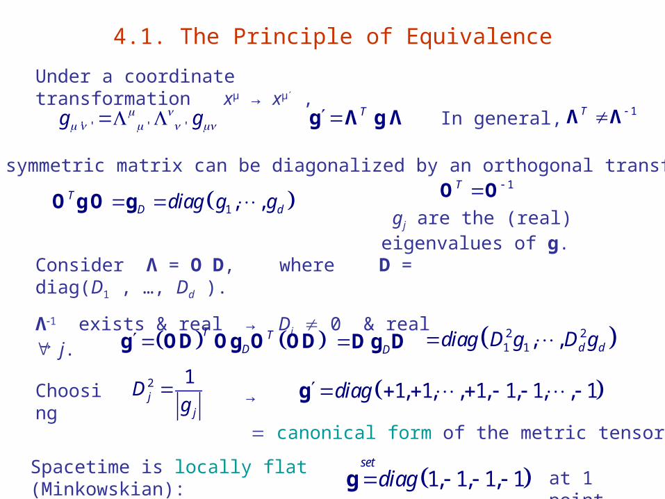
4.1. The Principle of Equivalence

Under a coordinate transformation xμ → xμ ,

' ' ' 'g g Tg Λ g Λ 1T Λ ΛIn general,

Every real symmetric matrix can be diagonalized by an orthogonal transformation:

1, ,TD ddiag g g O g O g

1T O O

gj are the (real) eigenvalues of g.

Consider Λ = O D, where D = diag(D1 , …, Dd ).

Λ1 exists & real → Dj 0 & real j.

2 21 1, , d ddiag D g D g T T

Dg OD Og O OD DD g D→

2 1j

j

DgChoosing → 1, 1, , 1, 1, 1, , 1diag g

canonical form of the metric tensor

Spacetime is locally flat (Minkowskian): 1, 1, 1, 1

set

diag g at 1 point.

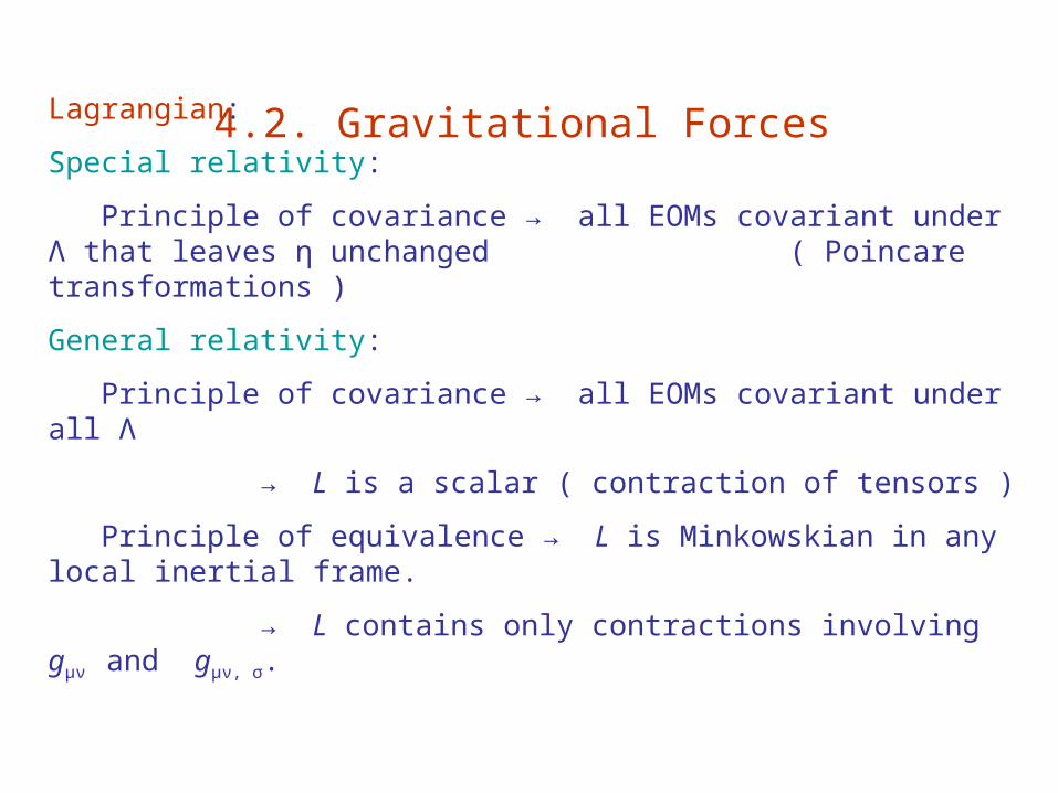
4.2. Gravitational ForcesLagrangian:

Special relativity:

Principle of covariance → all EOMs covariant under Λ that leaves η unchanged( Poincare transformations )

General relativity:

Principle of covariance → all EOMs covariant under all Λ

→ L is a scalar ( contraction of tensors )

Principle of equivalence → L is Minkowskian in any local inertial frame.

→ L contains only contractions involving gμν and gμν, σ.

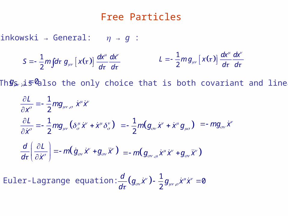
Free Particles

Minkowski → General: → g :

1

2

dx dxL m g x

d d

1

2

dx dxS m d g x

d d

; 0g → This is also the only choice that is both covariant and linear in g.

,

1

2

Lmg x x

x

1

2

Lmg x x

x

1

2m g x x g

mg x

d Lm g x g x

d x

,m g x x g x

,

10

2

dg x g x x

d

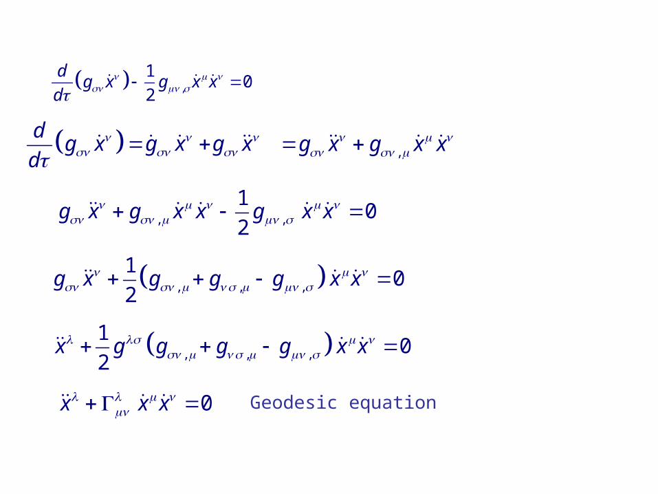
Euler-Lagrange equation:

,

10

2

dg x g x x

d

dg x g x g x

d

,g x g x x

, ,

10

2g x g x x g x x

, , ,

10

2g x g g g x x

, , ,

10

2x g g g g x x

0x x x Geodesic equation

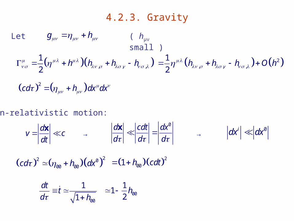
4.2.3. Gravity

g h Let ( hμν small )

, , ,

1

2h h h h

2, , ,

1

2h h h O h

2cd h dx dx

Non-relativistic motion:

dv c

dt

x

0d cdt dx

d d d

x→

0idx dx→

22 000 00cd h dx 2001 h cdt

00

1

1

dtt

d h

00

11

2h

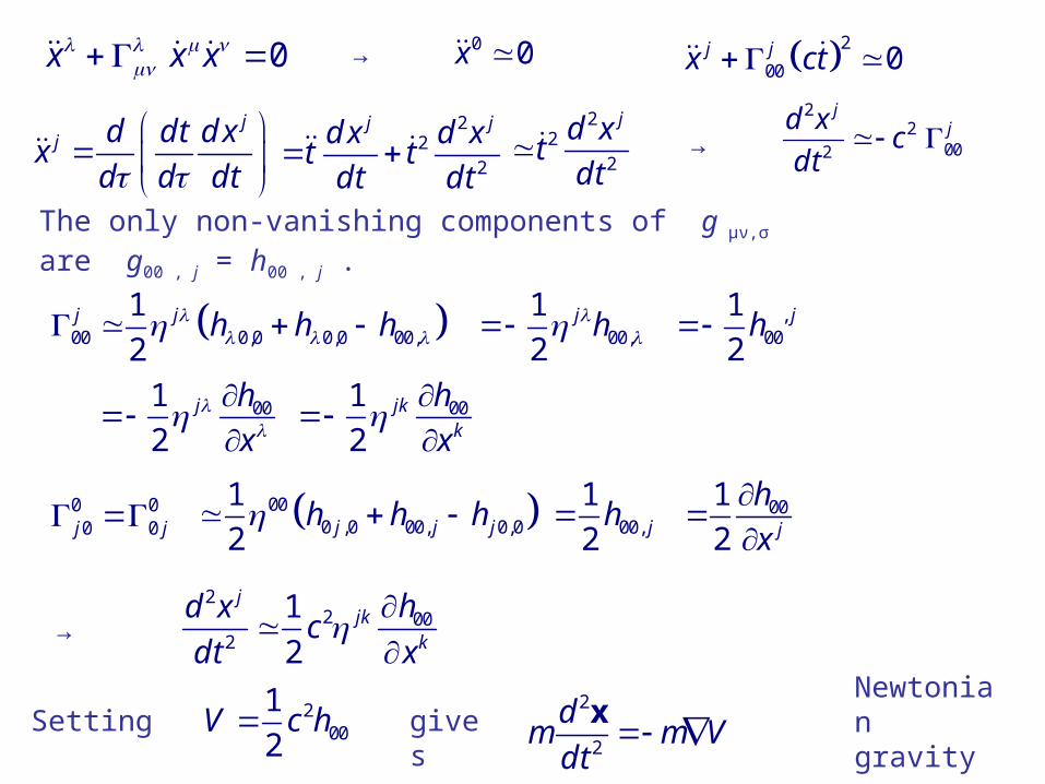
0x x x 0 0x 200 0j jx ct →

jj d dt d x

xd d dt

2

22

j jd x d xt t

dt dt

22

2

jd xt

dt

22

002

jjd x

cdt

→

The only non-vanishing components of g μν,σ are g00 , j = h00 , j .

00 0,0 0,0 00,

1

2j j h h h

00,

1

2j h ,

00

1

2jh

001

2j h

x

001

2jk

k

h

x

0 00 0j j 00

0 ,0 00, 0,0

1

2 j j jh h h 00,

1

2 jh 001

2 j

h

x

22 00

2

1

2

jjk

k

hd xc

dt x

→

Setting 200

1

2V c h

2

2

dm m V

dt

xgivesNewtonian gravity

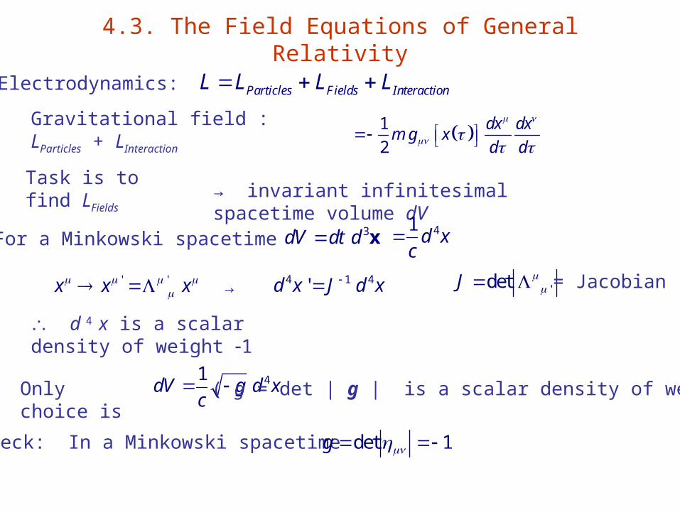
4.3. The Field Equations of General Relativity

Electrodynamics: Particles Fields InteractionL L L L

Gravitational field : LParticles + LInteraction 1

2

dx dxm g x

d d

Task is to find LFields → invariant infinitesimal spacetime volume dV

For a Minkowski spacetime 3dV dt d x 41d x

c

' 'x x x 4 1 4'd x J d x 'detJ

→ = Jacobian

d 4 x is a scalar density of weight 1

Only choice is41

dV g d xc ( g = det | g | is a scalar density of weight +2 )

Check: In a Minkowski spacetime det 1g

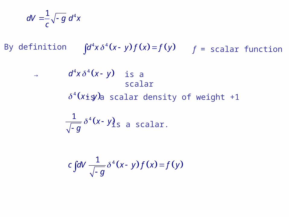
41dV g d x

c

By definition 4 4d x x y f x f y f = scalar function

4 4d x x y

4 x y

→ is a scalar

is a scalar density of weight +1

41x y

g

is a scalar.

41c dV x y f x f y

g

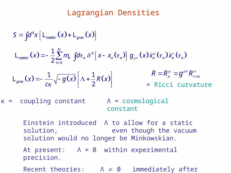
Lagrangian Densities

4matter gravS d x x x L L

4

1

1

2

N

matter n n n n n n n nn

x m d x x g x x x

L

1 1

2grav x g x R xc

L

R R g R

= Ricci curvature

κ = coupling constant Λ = cosmological constant

Einstein introduced Λ to allow for a static solution, even though the vacuum solution would no longer be Minkowskian.

At present: Λ = 0 within experimental precision.

Recent theories: Λ 0 immediately after the Big Bang.

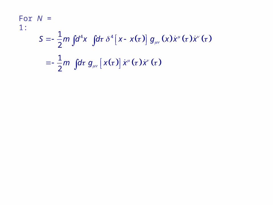
For N = 1:

4 41

2S m d x d x x g x x x

1

2m d g x x x

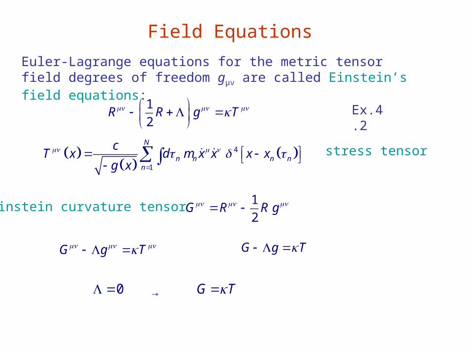
Field Equations

Euler-Lagrange equations for the metric tensor field degrees of freedom gμν are called Einstein’s field equations:

1

2R R g T

4

1

N

n n n nn

cT x d m x x x x

g x

1

2G R R g

G g T G g T

stress tensor

Einstein curvature tensor

0 G T→

Ex.4.2

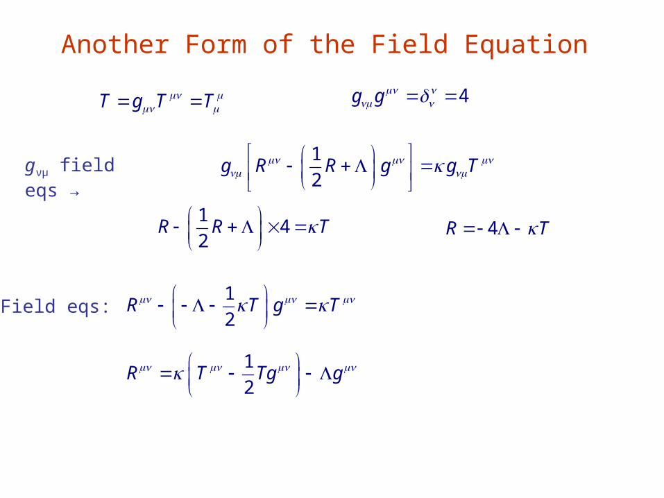
Another Form of the Field Equation

T g T T 4g g

1

2g R R g g T

14

2R R T

4R T

1

2R T g T

1

2R T Tg g

gνμ field eqs →

Field eqs:

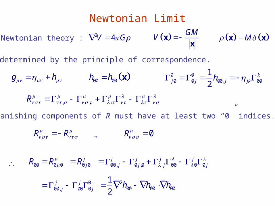
Newtonian Limit

Newtonian theory : 2 4V G GMV x

x M x x

κ is determined by the principle of correspondence.

g h 00 00h h x 0 00 0 00, 00

1

2k

j j j jkh

, ,R

R R 0R

00 0 0R R 0 0jjR 00, 0 ,0 00 0 0

j j j jj j j j

→ non-vanishing components of R must have at least two “0” indices.

→

000, 00 0j j

j j 200 00 00

1

2h h h

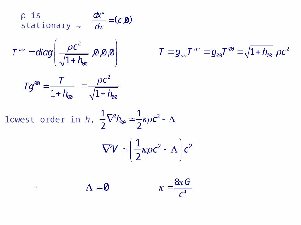
ρ is stationary → ,dx

cd

0

2

00

,0,0,01

cT diag

h

00 200 001T g T g T h c

00

001

TTg

h

2

001

c

h

To lowest order in h, 2 200

1 1

2 2h c

2 2 21

2V c c

4

8 G

c

→ 0

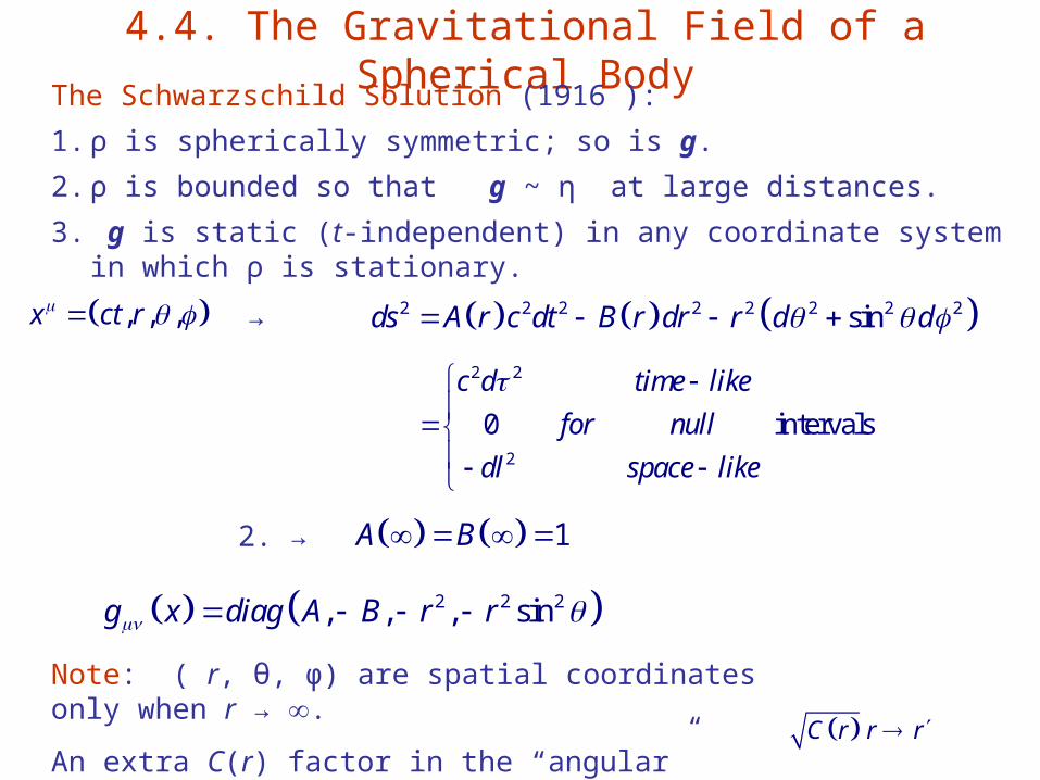
4.4. The Gravitational Field of a Spherical Body

The Schwarzschild Solution (1916 ):

1. ρ is spherically symmetric; so is g.

2. ρ is bounded so that g ~ η at large distances.

3. g is static (t-independent) in any coordinate system in which ρ is stationary.

, , ,x ct r 2 2 2 2 2 2 2 2sinds A r c dt B r dr r d d

1A B 2. →

Note: ( r, θ, φ) are spatial coordinates only when r → .

An extra C(r) factor in the “angular” term can be absorbed by C r r r

→

2 2 2, , , sing x diag A B r r

2 2

2

0 intervals

c d time like

for null

dl space like

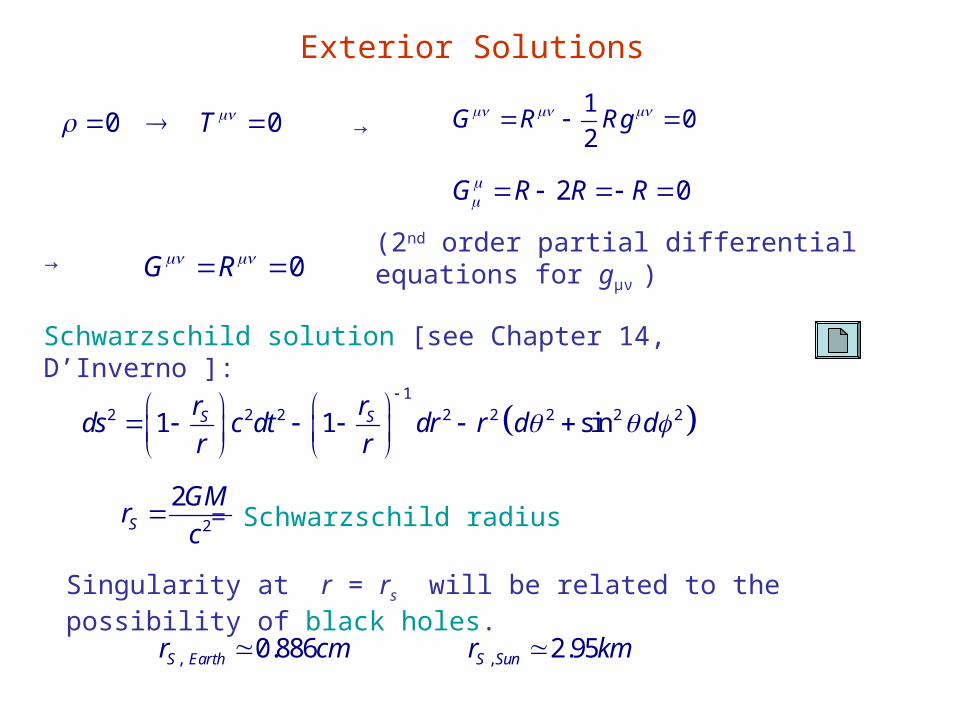
Exterior Solutions

0 0T 1

02

G R Rg →

2 0G R R R

0G R (2nd order partial differential equations for gμν )→

Schwarzschild solution [see Chapter 14, D’Inverno ]:

1

2 2 2 2 2 2 2 21 1 sinS Sr rds c dt dr r d d

r r

2

2S

GMr

c = Schwarzschild radius

Singularity at r = rs will be related to the possibility of black holes.

, 0.886S Earthr cm , 2.95S Sunr km

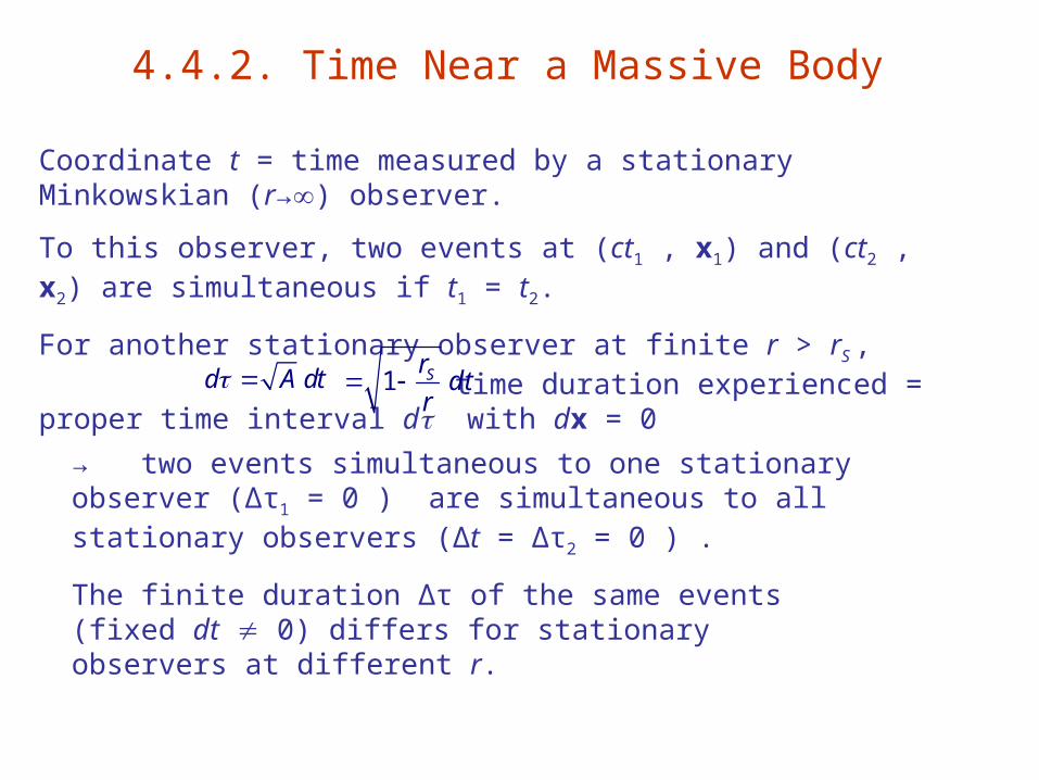
4.4.2. Time Near a Massive Body

Coordinate t = time measured by a stationary Minkowskian (r→) observer.

To this observer, two events at (ct1 , x1) and (ct2 , x2) are simultaneous if t1 = t2.

For another stationary observer at finite r > rS , time duration experienced = proper time interval d with dx = 0

d A dt 1 Sr dtr

→ two events simultaneous to one stationary observer (Δτ1 = 0 ) are simultaneous to all stationary observers (Δt = Δτ2 = 0 ) .

The finite duration Δτ of the same events (fixed dt 0) differs for stationary observers at different r.

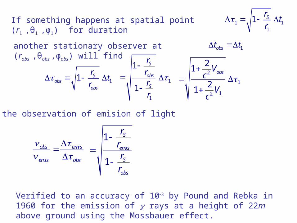
If something happens at spatial point (r1 ,θ1 ,φ1) for duration 1 11

1 Sr tr

another stationary observer at (robs ,θobs ,φobs) will find 1obst t

11 Sobs

obs

rt

r 1

1

1

1

S

obs

S

rrrr

2

1

12

21

21

obsVc

Vc

For the observation of emision of light

obs emis

emis obs

1

1

S

emis

S

obs

rrrr

Verified to an accuracy of 103 by Pound and Rebka in 1960 for the emission of rays at a height of 22m above ground using the Mossbauer effect.

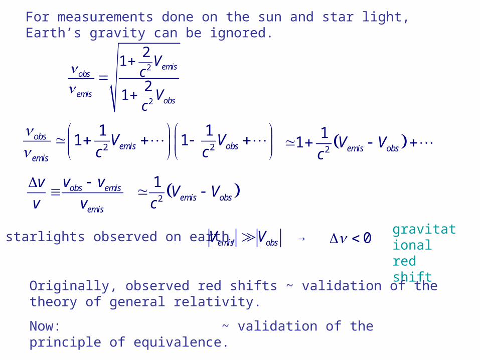
For measurements done on the sun and star light, Earth’s gravity can be ignored.

2

2

21

21

emisobs

emisobs

Vc

Vc

2 2

1 11 1obs

emis obsemis

V Vc c

2

11 emis obsV V

c

obs emis

emis

v v v

v v

2

1emis obsV V

c

For starlights observed on earth, emis obsV V 0 →gravitational red shift

Originally, observed red shifts ~ validation of the theory of general relativity.

Now: ~ validation of the principle of equivalence.

→ Allows for other gravitational theories, such as the Brans-Dicke theory.

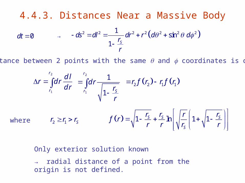
4.4.3. Distances Near a Massive Body

2 2 2 2 2 2 21sin

1 S

ds dl dr r d dr

r

0dt →

Radial distance between 2 points with the same and coordinates is defined as

2

1

r

r

d lr d r

d r

2

1

1

1

r

r S

d rr

r

2 2 1 1r f r r f r

2 1 Sr r r 1 ln 1 1S S S

S

r r r rf r

r r r r

where

Only exterior solution known

→ radial distance of a point from the origin is not defined.

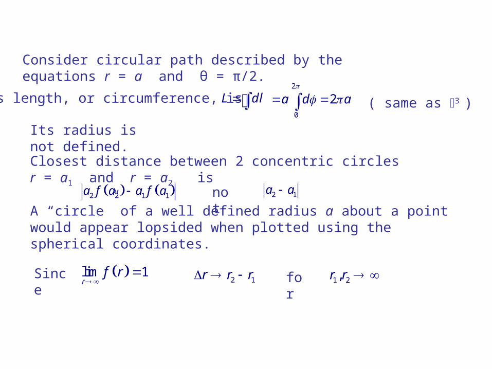
Consider circular path described by the equations r = a and θ = π/2.

Its length, or circumference, is L dl2

0

2a d a

( same as 3 )

Its radius is not defined.Closest distance between 2 concentric circles r = a1 and r = a2 is

2 2 1 1a f a a f a not 2 1a a

A “circle” of a well defined radius a about a point would appear lopsided when plotted using the spherical coordinates.

Since lim 1r

f r

2 1r r r 1 2,r r

for

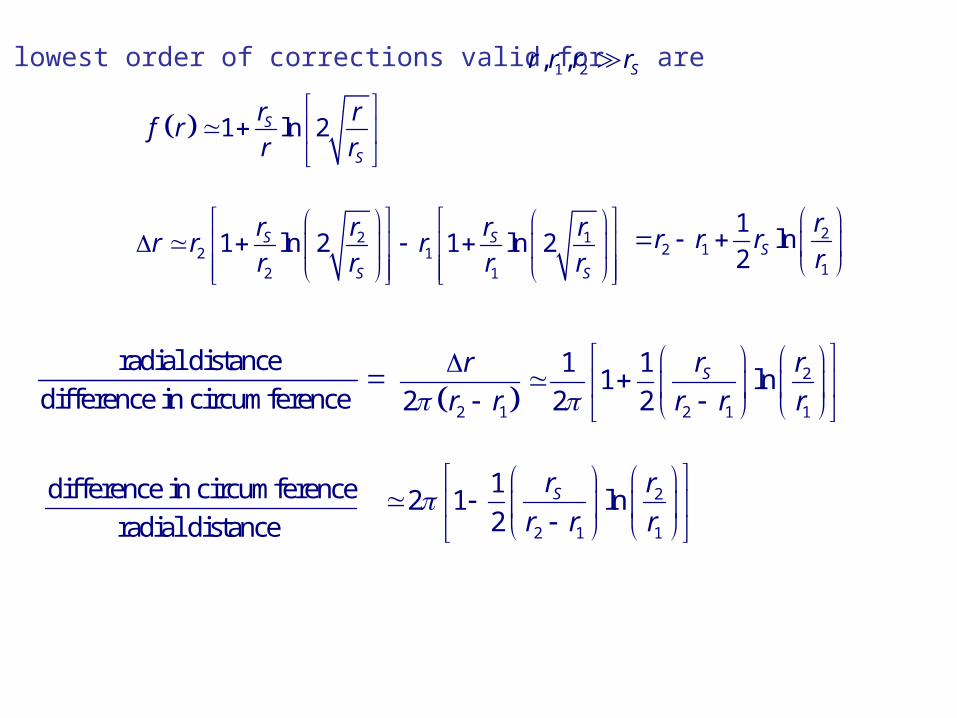
The lowest order of corrections valid for 1 2, , Sr r r r are

1 ln 2S

S

r rf r

r r

2 12 1

2 1

1 ln 2 1 ln 2S S

S S

r r r rr r r

r r r r

2

2 11

1ln

2 S

rr r r

r

radial distance

difference in circumference

2

2 1 2 1 1

1 11 ln

2 2 2Sr r r

r r r r r

difference in circumference

radial distance 2

2 1 1

12 1 ln

2Sr r

r r r

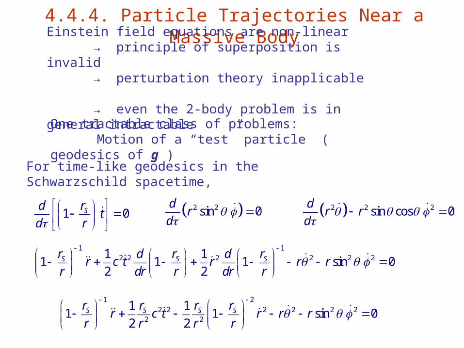
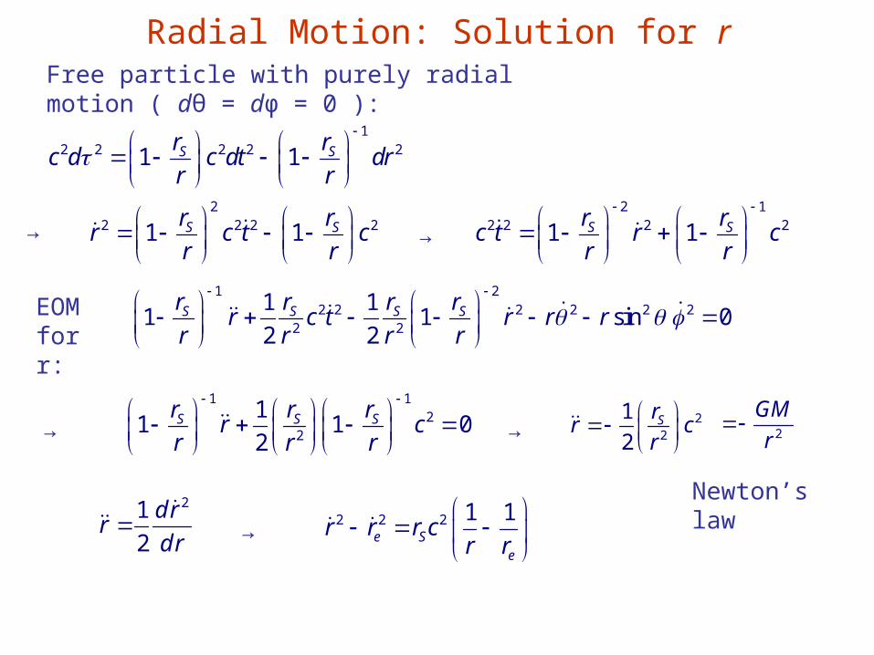
4.4.4. Particle Trajectories Near a Massive Body

Einstein field equations are non-linear → principle of superposition is invalid → perturbation theory inapplicable → even the 2-body problem is in general intractable

One tractable class of problems:Motion of a “test” particle ( geodesics of g )

For time-like geodesics in the Schwarzschild spacetime,

1 0Sd rt

d r

2 2 2sin cos 0d

r rd

2 2sin 0d

rd

1 12 2 2 2 2 21 1

1 1 1 sin 02 2

S S Sr d r d rr c t r r r

r dr r dr r

1 22 2 2 2 2 2

2 2

1 11 1 sin 0

2 2S S S Sr r r r

r c t r r rr r r r

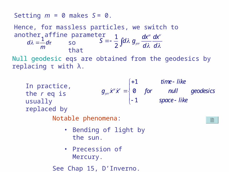
Setting m = 0 makes S = 0.

Hence, for massless particles, we switch to another affine parameter

1d d

m so that

1

2

dx dxS d g

d d

Null geodesic eqs are obtained from the geodesics by replacing τ with λ.

Notable phenomena:

• Bending of light by the sun.

• Precession of Mercury.

See Chap 15, D’Inverno.

In practice, the r eq is usually replaced by

1

0

1

time like

g x x for null geodesics

space like

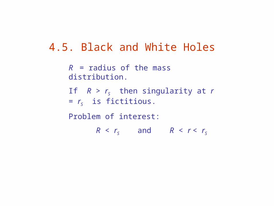
4.5. Black and White Holes

R = radius of the mass distribution.

If R > rS then singularity at r = rS is fictitious.

Problem of interest:

R < rS and R < r < rS

Radial Motion: Solution for r

Free particle with purely radial motion ( dθ = dφ = 0 ):

12 2 2 2 21 1S Sr r

c d c dt drr r

22 2 2 21 1S Sr r

r c t cr r

2 1

2 2 2 21 1S Sr rc t r c

r r

→ →

EOM for r:

1 12

2

11 1 0

2S S Sr r r

r cr r r

→2

2

1

2Srr c

r

2

GM

r

21

2

d rr

d r

2 2 2 1 1

e Se

r r r cr r

→

1 22 2 2 2 2 2

2 2

1 11 1 sin 0

2 2S S S Sr r r r

r c t r r rr r r r

→

Newton’s law

ForS

ee

rr c

r we have

22 Sr c

rr

→S

rdr cd

r

3/ 2 3/ 20

2

3 S

r r cr

0 0r r

2 / 3

3/ 20

3

2 Sr r r c →

Outgoing Incoming

Singularity at r = rS not felt

2 2 2 1 1e S

e

r r r cr r

Radial Motion: Solution for t 2

2 Sr cr

r

2 12 2 2 21 1S Sr r

c t r cr r

Putting into

gives

22 2 2 21 1S S Sr r r

c c t cr r r

221 1Sr t

r

1

1 S

trr

→ →

dt d rt

d r d

dtr

d r Srdt

cd r r

1

1

S

S

rdtc

rd r rr

→

→ Outgoing Incoming

for r > rS

Incoming Outgoing

for r < rS

3/ 2

SS

dt rc r

d r r r

3/ 2

SS

dt rc r

d r r r →

3/ 21

SS

rc t dr

r rr

3/ 2 3/ 2 11 22 2 tanh

3S SSS

rct r r r r

rr

3/ 2 3/ 2

11 2

2 ln3

1

SS S

S

S

rr

r r r rr r

r

3/ 2 3/ 2

11 2

2 ln3

1

SS S

S

S

rr

ct r r r rr r

r

3/ 2 3/ 20

2

3S

S

r rc r

For an incoming particle in the region r > rS

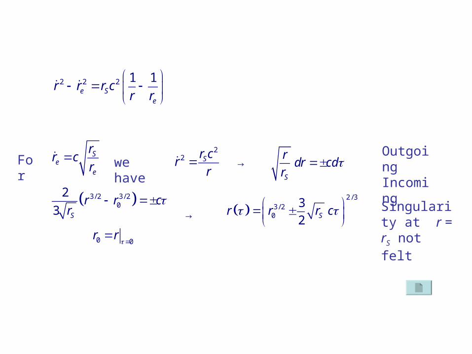
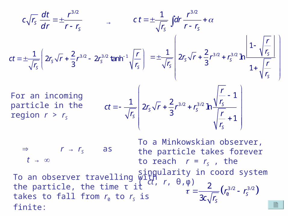
r → rS as t → To a Minkowskian observer, the particle takes forever to reach r = rS , the singularity in coord system ( ct, r, θ,φ)

To an observer travelling with the particle, the time τ it takes to fall from r0 to rS is finite:

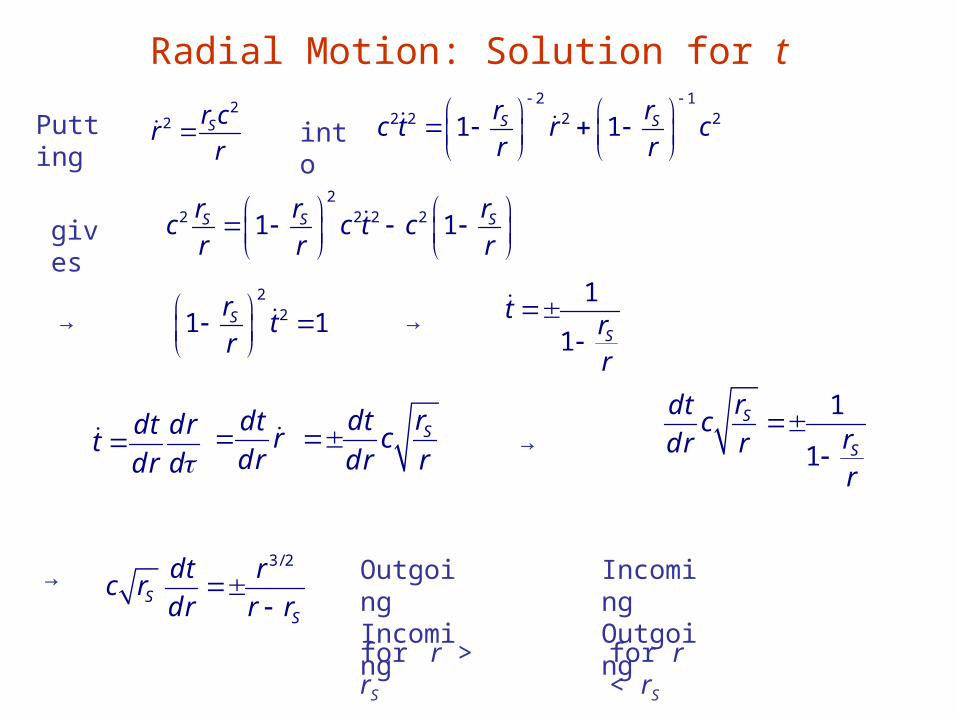
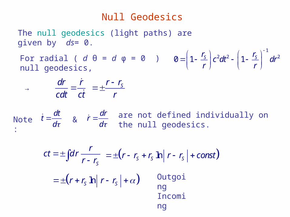
Null Geodesics

The null geodesics (light paths) are given by ds= 0.

For radial ( d θ = d φ = 0 ) null geodesics, 1

2 2 20 1 1S Sr rc dt dr

r r

→dr r

cdt ct

Sr r

r

Note:

dtt

d

drr

d are not defined individually on the null geodesics.&

S

rct d r

r r

lnS S Sr r r r r const

lnS Sr r r r Outgoing Incoming

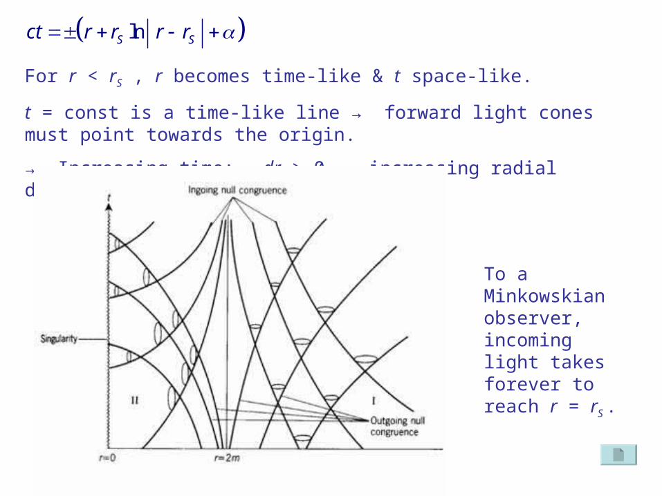
For r < rS , r becomes time-like & t space-like.

t = const is a time-like line → forward light cones must point towards the origin.

→ Increasing time: dr > 0, increasing radial distance: c dt > 0.

lnS Sct r r r r

To a Minkowskian observer, incoming light takes forever to reach r = rS .

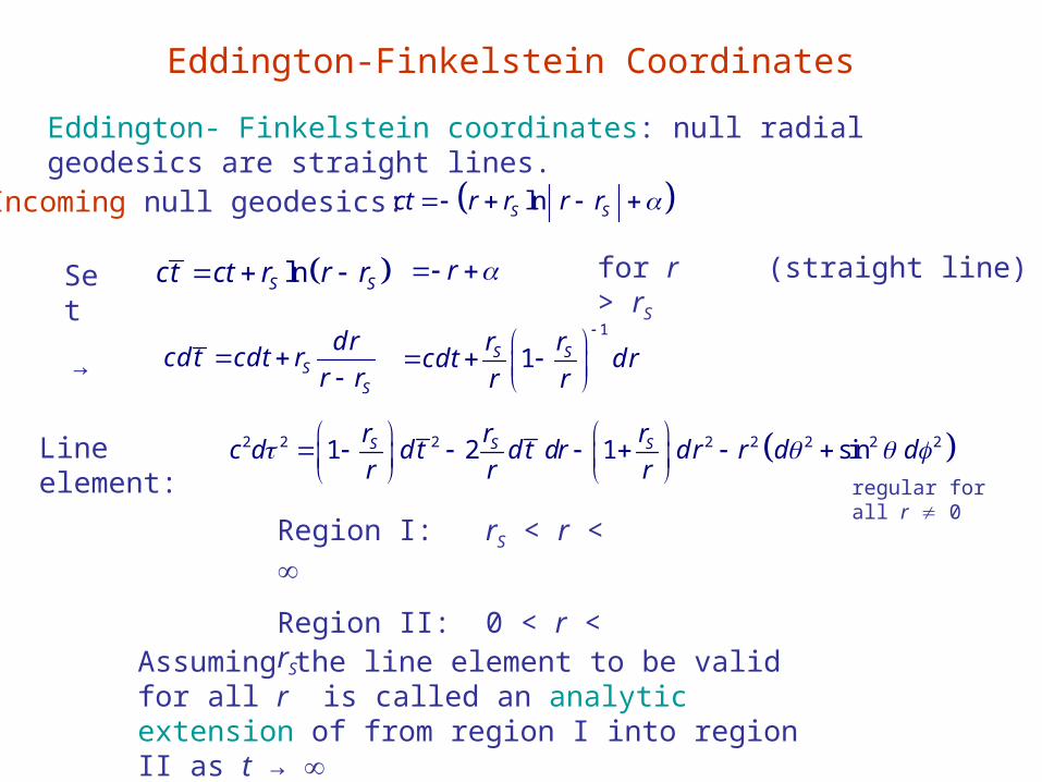
Eddington-Finkelstein Coordinates

Eddington- Finkelstein coordinates: null radial geodesics are straight lines.Incoming null geodesics: lnS Sct r r r r

Set lnS Sct ct r r r r for r > rS (straight line)

→ SS

d rcd t cdt r

r r

1

1S Sr rcdt d r

r r

Line element:

2 2 2 2 2 2 2 21 2 1 sinS S Sr r rc d d t d t dr d r r d d

r r r

regular for all r 0

Region I: rS < r <

Region II: 0 < r < rS

Assuming the line element to be valid for all r is called an analytic extension of from region I into region II as t →

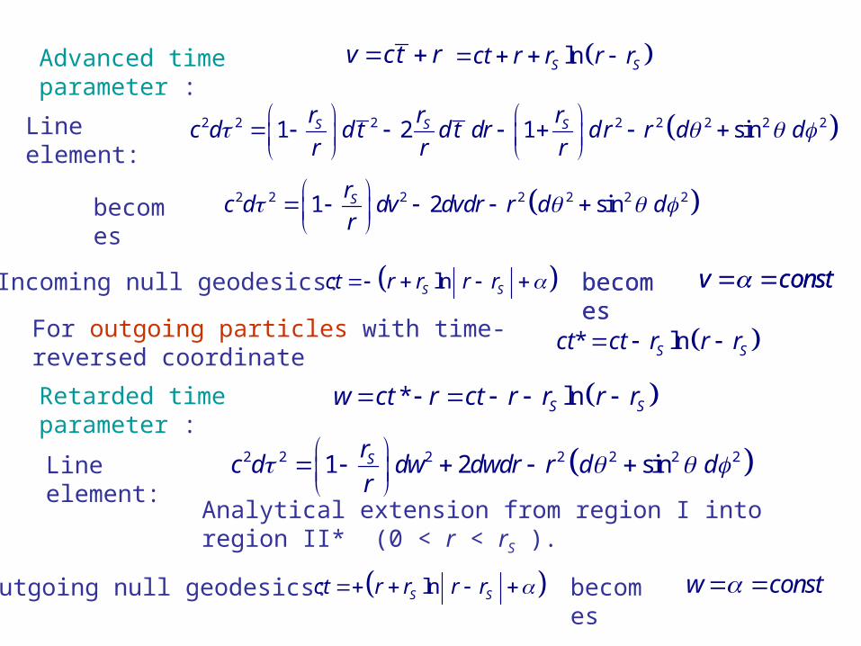
Advanced time parameter : v ct r lnS Sct r r r r

2 2 2 2 2 2 21 2 sinSrc d dv dvdr r d dr

Line element:

Incoming null geodesics: v const

2 2 2 2 2 2 2 21 2 1 sinS S Sr r rc d d t d t dr d r r d d

r r r

becomes

lnS Sct r r r r becomes

For outgoing particles with time-reversed coordinate

* lnS Sct ct r r r

Retarded time parameter : * lnS Sw ct r ct r r r r

Line element:

2 2 2 2 2 2 21 2 sinSrc d dw dwdr r d dr

Analytical extension from region I into region II* (0 < r < rS ).

Outgoing null geodesics: lnS Sct r r r r

v const becomes

w const becomes

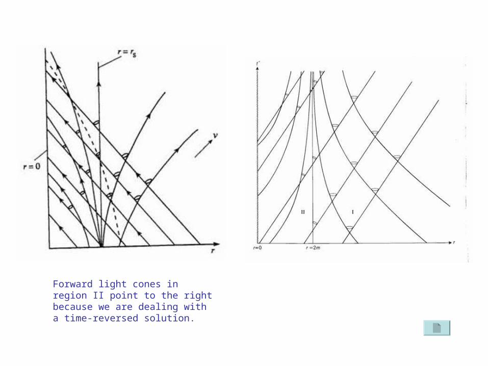
Forward light cones in region II point to the right because we are dealing with a time-reversed solution.

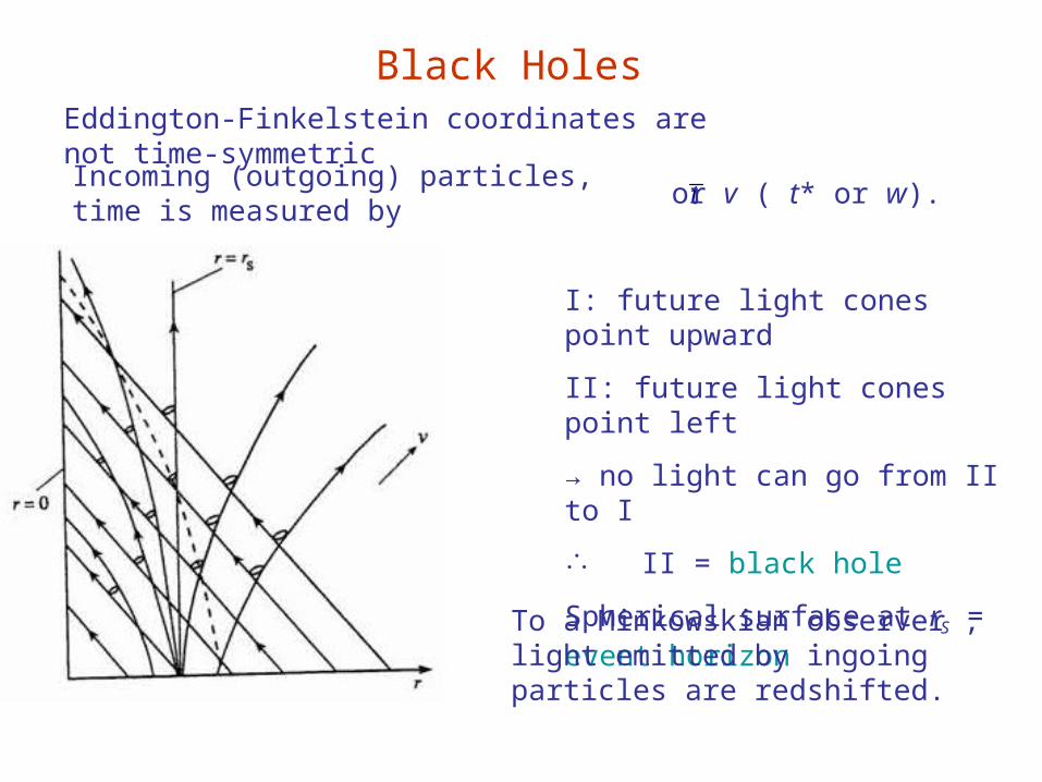
Black Holes

Eddington-Finkelstein coordinates are not time-symmetric

Incoming (outgoing) particles, time is measured by t or v ( t* or w).

I: future light cones point upward

II: future light cones point left

→ no light can go from II to I

II = black hole

Spherical surface at rS = event horizon

To a Minkowskian observer , light emitted by ingoing particles are redshifted.

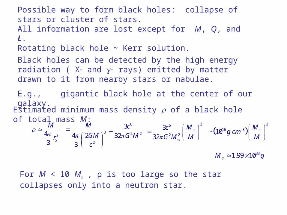
Possible way to form black holes: collapse of stars or cluster of stars.All information are lost except for M, Q, and L. Rotating black hole ~ Kerr solution.

Black holes can be detected by the high energy radiation ( X and rays) emitted by matter drawn to it from nearby stars or nabulae.

E.g., gigantic black hole at the center of our galaxy.

Estimated minimum mass density of a black hole of total mass M:

343 S

M

r 3

2

4 23

M

GMc

6

2 2

3

32

c

G M

26

2 2

3

32

Mc

G M M

2

16 310M

g cmM

331.99 10M g

For M < 10 M , ρ is too large so the star collapses only into a neutron star.

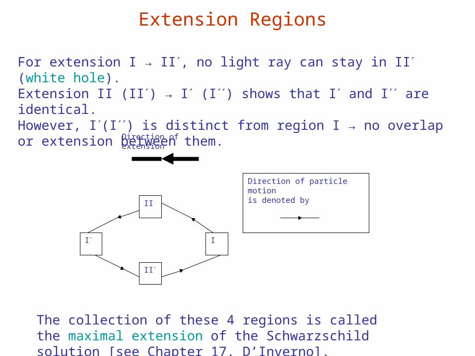
Extension Regions

II

I

II

I

Direction of extension

Direction of particle motionis denoted by

For extension I → II, no light ray can stay in II (white hole).Extension II (II) → I (I) shows that I and I are identical. However, I(I) is distinct from region I → no overlap or extension between them.

The collection of these 4 regions is called the maximal extension of the Schwarzschild solution [see Chapter 17, D’Inverno].