4 Molecular dynamics - University of Toronto · 2011-05-03 · 4 Molecular dynamics 4.1 Basic...

4

Molecular dynamics

4.1 Basic integration schemes

4.1.1 General concepts

• Aim of Molecular Dynamics (MD) simulations:compute equilibrium and transport properties of classical many body systems.

• Basic strategy: numerically solve equations of motions.

• For many classical systems, the equations of motion are of Newtonian form

RN =1

mPN

PN = FN = − ∂U

∂RN,

or

XN = LXN , with LA = {A,H},where XN = (RN , PN).

The energy H = P N ·P N

2m+ U(RN) is conserved under this dynamics.

The potential energy is typically of the form of a sum of pair potentials:

U(RN) =∑(i,j)

ϕ(rij) =N∑

i=1

i−1∑j=1

ϕ(rij),

which entails the following expression for the forces FN :

Fi = −∑j 6=i

∂

∂ri

ϕ(rij) = −∑j 6=i

ϕ′(rij)∂rij

∂ri

=∑j 6=i

ϕ′(rij)rj − ri

rij︸︷︷︸Fij

47

48 4. MOLECULAR DYNAMICS

• Examples of quantities of interest:

1. Radial distribution function (structural equilibrium property)

g(r) =2V

N(N − 1)

∑(i,j)

〈δ(ri − rj − r)〉 ,

where

〈A〉 =

∫dXN A(XN)e−βH(XN )∫

dXN e−βH(XN )(canonical ensemble)

or =

∫dXN A(XN) δ(E −H(XN))∫

dXN δ(E −H(XN))(microcanonical ensemble).

2. Pressure (thermodynamic equilibrium property):

pV = NkT +1

3

∑(i,j)

〈Fij · rij〉

which can be written in terms of g(r) as well.

3. Mean square displacement (transport property):⟨|r(t)− r(0)|2

⟩→ 6Dt for long times t,

where D is the self diffusion coefficient.

4. Time correlation function (relaxation properties)

C(t) = 〈v(t) · v(0)〉

which is related to D as well:

D =1

3limt→∞

limN,V→∞

∫ t

0

C(τ) dτ

• If the system is ergodic then time average equals the microcanonical average:

limtfinal→∞

1

tfinal

∫ tfinal

0

dt A(XN(t)) =

∫dXN A(XN) δ(E −H(XN))∫

dXN δ(E −H(XN)).

• For large N , microcanonical and canonical averages are equal for many quantities A.

• Need long times tfinal!

4.1. BASIC INTEGRATION SCHEMES 49

• The equations of motion to be solved are ordinary differential equations.

• There exist general algorithms to solve ordinary differential equations numerically (seee.g. Numerical Recipes Ch. 16), such as Runge-Kutta and predictor/correction algo-rithms. Many of these are too costly or not stable enough for long simulations ofmany-particle systems. In MD simulations, it is therefore better to use algorithmsspecifically suited for systems obeying Newton’s equations of motion, such as the Ver-let algorithm.

• However, we first want to explore some general properties of integration algorithms.For this purpose, consider a function x of t which satisfies

x = f(x, t). (4.1)

• We want to solve for the trajectory x(t) numerically, given the initial point x(0) attime t = 0.

• Similar to the case of integration, we restrict ourselves to a discrete set of points,separated by a small time step ∆t:

tn = n∆t

xn = x(tn),

where n = 0, 1, 2, 3, . . . .

• To transform equation (4.1) into a closed set of equations for the xn, we need to expressthe time derivative x in terms of the xn. This can only be done approximately.

• Using that ∆t is small:

x(tn) ≈ x(tn + ∆t)− x(tn)

∆t=

xn+1 − xn

∆t.

• Since this should be equal to f(x(t), t) = f(xn, tn):

xn+1 − xn

∆t≈ f(xn, tn) ⇒

xn+1 = xn + f(xn, tn)∆t Euler Scheme. (4.2)

This formula allows one to generate a time series of points which are an approximationto the real trajectory. A simple MD algorithm in pseudo-code could look like this:1

1Pseudo-code is an informal description of an algorithm using common control elements found in mostprogramming language and natural language; it has no exact definition but is intended to make implemen-tation in a high-level programming language straightforward.


EULER ALGORITHM

SET x to the initial value x(0)

SET t to the initial time

WHILE t < tfinal

COMPUTE f(x,t)

UPDATE x to x+f(x,t)*dt

UPDATE t to t+dt

END WHILE

DO NOT USE THIS ALGORITHM!

• It is easy to show that the error in the Euler scheme is of order ∆t2, since

x(t + ∆t) = x(t) + f(x(t), t)∆t +1

2x(t)∆t2 + . . . ,

so that

xn+1 = xn + f(xn, tn)∆t +O(∆t2)︸︷︷︸local error

. (4.3)

The strict meaning of the “big O” notation is that if A = O(∆tk) then lim∆t→0 A/∆tk

is finite and nonzero. For small enough ∆t, a term O(∆tk+1) becomes smaller thana term O(∆tk), but the big O notation cannot tell us what magnitude of ∆t is smallenough.

• A numerical prescription such as (4.3) is called an integration algorithm, integrationscheme, or integrator.

• Equation (4.3) expresses the error after one time step; this is called the local truncationerror.

• What is more relevant is the global error that results after a given physical time tf oforder one. This time requires M = tf/∆t MD steps to be taken.

• Denoting fk = f(xk, tk), we can track the errors of subsequent time steps as follows:

x1 = x0 + f0∆t +O(∆t2)

x2 = [x0 + f0∆t +O(∆t2)] + f1∆t +O(∆t2)

= x0 + (f0 + f1)∆t +O(∆t2) +O(∆t2)

...

xM = x0 +M∑

k=1

fk−1∆t +M∑

k=1

O(∆t2);


but as M = tf/∆t:

x(t) = xM = x0 +

tf /∆t∑k=1

fk−1∆t +

tf /∆t∑k=1

O(∆t2)︸︷︷︸global error

.

• Since tf = O(1), the accumulated error is

tf /∆t∑k=1

O(∆t2) = O(∆t2)O(tf/∆t) = O(tf∆t), (4.4)

which is of first order in the time step ∆t.

• Since the global error goes as the first power of the time step ∆t, we call equation (4.3)a first order integrator.

• In absence of further information on the error terms, this constitutes a general principle:If in a single time step of an integration scheme, the local truncation error is O(∆tk+1),then the globally accumulated error over a time tf is O(tf∆tk) = O(∆tk), i.e., thescheme is kth order.

• Equation (4.4) also shows the possibility that the error grows with physical time tf :Drift.

• Illustration of local and global errors:Let f(x, t) = −αx, so that equation (4.1) reads

x = −αx,

whose solution is exponentially decreasing with a rate α:

x(t) = e−αtx(0). (4.5)

The numerical scheme (4.3) gives for this system

xn+1 = xn − αxn∆t. (4.6)

Note that the true relation is x(t + ∆t) = e−α∆tx(t) = x(t) − α∆tx(t) +O(∆t2), i.e.,the local error is of order ∆t2.

Equation (4.6) is solved by

xn = (1− α∆t)nx0 = (1− α∆t)t/∆t = e[ln(1−α∆t)/∆t]t. (4.7)


By comparing equations (4.5) and (4.7), we see that the behaviour of the numericalsolution is similar to that of the real solution but with the rate α replaced by α′ =− ln(1−α∆t)/∆t. For small ∆t, one gets for the numerical rate α′ = α+α2∆t/2+· · · =α+O(∆t), thus the global error is seen to be O(∆t), which demonstrates that the Eulerscheme is a first order integrator. Note that the numerical rate diverges at ∆t = 1/α,which is an example of a numerical instability.

4.1.2 Ingredients of a molecular dynamics simulation

1. Boundary conditions

• We can only simulate finite systems.

• A wall potential would give finite size effects and destroy translation invariance.

• More benign boundary conditions: Periodic Boundary Conditions:

• Let all particles lie in a simulation box with coordinates between −L/2 and L/2.

• A particle which exits the simulation box, is put back at the other end.

• Infinite checkerboard picture (easiest to visualize in two dimensions):

• The box with thick boundaries is our simulation box.

• All other boxes are copies of the simulation box, called periodic images.

• The other squares contain particles with shifted positions

r′ = r +

iLjLkL

,

for any negative or positive integers i, j, and k. Thus, if a particle moves out ofthe simulation box, another particle will fly in from the other side.


Conversely, for any particle at position r′ not in the simulation box, there is aparticle in the simulation box at

r =

(x′ + L2) mod L− L

2

(y′ + L2) mod L− L

2

(z′ + L2) mod L− L

2

, (4.8)

• Yet another way to view this is to say that the system lives on a torus.

2. Forces

• Usually based on pair potentials.

• A common pair potential is the Lennard-Jones potential

ϕ(r) = 4ε

[(σ

r

)12

−(σ

r

)6]

,

– σ is a measure of the range of the potential.

– ε is its strength.

– The potential is positive for small r: repulsion.

– The potential is negative for large r: attraction.

– The potential goes to zero for large r: short-range.

– The potential has a minimum of −ε at 21/6σ.

• Computing all forces in an N-body system requires the computation of N(N−1)/2(the number of pairs in the system) forces Fij

• Computing forces is often the most demanding part of MD simulations.

• A particle i near the edge of the simulation box will feel a force from the periodicimages, which can be closer to i than their original counter-parts.

• A consistent way to write the potential is

U =∑i,j,k

N∑n=1

n−1∑m=1

ϕ(|rn − rm + iLx + jLy + kLz|). (4.9)

• While this converges for most potentials ϕ, it is very impractical to have to com-pute an infinite sum to get the potential and forces.

• To fix this, one can modify the potential such that it becomes zero beyond acertain cut-off distance rc:

ϕ′(r) =

{ϕ(r)− ϕ(rc) if r < rc

0 if r ≥ rc

where the subtraction of ϕ(rc) is there to avoid discontinuities in the potentialwhich would cause violations of energy conservation.


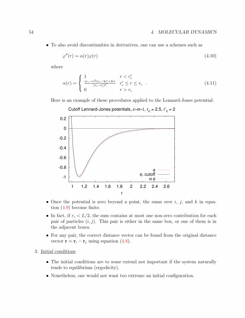
• To also avoid discontinuities in derivatives, one can use a schemes such as

ϕ′′(r) = α(r)ϕ(r) (4.10)

where

α(r) =

1 r < r′c(rc−r)2(rc−3r′c+2r)

(rc−r′c)3 r′c ≤ r ≤ rc

0 r > rc

. (4.11)

Here is an example of these procedures applied to the Lennard-Jones potential:

-1

-0.8

-0.6

-0.4

-0.2

0

0.2

1 1.2 1.4 1.6 1.8 2 2.2 2.4 2.6r

Cutoff Lennard-Jones potentials, ε=σ=1, rc = 2.5, r’c = 2

φφ, cutoff

α φ

• Once the potential is zero beyond a point, the sums over i, j, and k in equa-tion (4.9) become finite.

• In fact, if rc < L/2, the sum contains at most one non-zero contribution for eachpair of particles (i, j). This pair is either in the same box, or one of them is inthe adjacent boxes.

• For any pair, the correct distance vector can be found from the original distancevector r = ri − rj using equation (4.8).

3. Initial conditions

• The initial conditions are to some extend not important if the system naturallytends to equilibrium (ergodicity).

• Nonetheless, one would not want too extreme an initial configuration.


• Starting the system with the particles on a lattice and drawing initial momentafrom a uniform or Gaussian distribution is typically a valid starting point.

• One often makes sure that the kinetic energy has the target value 32NkT , while

the total momentum is set to zero to avoid the system moving as a whole.

4. Integration scheme

• Needed to solve the dynamics as given by the equations of motion.

• Below, we will discuss in detail on how to construct or choose an appropriateintegration scheme.

5. Equilibration/Burn-in

• Since we do not start the system from an equilibrium state, a certain number oftime steps are to be taken until the system has reached an equilibrium.

• One can check for equilibrium by seeing if quantities like the potential energy areno longer changing in any systematic fashion and are just fluctuating around amean values.

• The equilibrium state is microcanonical at a given total energy Etot = Epot +Ekin.

• Since Ekin > 0, the lattice initialization procedure outlined cannot reach all pos-sible values of the energy, i.e. Etot > Epot(lattice).

• To reach lower energies, one can periodically rescale the momenta (a rudimentaryform of a so called thermostat).

• Another way to reach equilibrium is to generate initial conditions using the MonteCarlo method.

6. Measurements

• Construct estimators for physical quantities of interest.

• Since there are correlations along the simulated trajectory, one needs to takesample points that are far apart in time.

• Although when one is interested in dynamical quantities, all points should beused. In the statistical analysis there correlations should be taken into account.


Given these ingredients, the outline of an MD simulation could look like this:

OUTLINE MD PROGRAM

SETUP INITIAL CONDITIONS

PERFORM EQUILIBRATION by INTEGRATING over a burn-in time B

SET time t to 0

PERFORM first MEASUREMENT

WHILE t < tfinal

INTEGRATE over the measurement interval

PERFORM MEASUREMENT

END WHILE

in which the integration step from t1 to t1+T looks as follows (assuming t=t1 at the start):

OUTLINE INTEGRATION

WHILE t < t1+T

COMPUTE FORCES on all particles

COMPUTE new positions and momenta according to INTEGRATION SCHEME

APPLY PERIODIC BOUNDARY CONDITIONS

UPDATE t to t+dt

END WHILE

Note: we will encounter integration schemes in which the forces need to be computed inintermediate steps, in which case the separation between force computation and integrationis not as strict as this outline suggests.

4.1.3 Desirable qualities for a molecular dynamics integrator

• Accuracy:Accuracy means that the trajectory obeys the equations of motion to good approxima-tion. This is a general demand that one would also impose on integrators for generaldifferential equations. The accuracy in principle improves by decreasing the time step∆t. But because of the exponential separation of near-by trajectories in phase space(Lyapunov instability), this is of limited help.

Furthermore, one cannot decrease ∆t too far in many particle systems for reasons of

• Efficiency:

It is typically quite expensive to compute the inter-particle forces FN , and takingsmaller time steps ∆t requires more force evaluations per unit of physical time.


• Respect physical laws:

– Time reversal symmetry

– Conservation of energy

– Conservation of linear momentum

– Conservation of angular momentum

– Conservation of phase space volume

provided the simulated system also has these properties, of course.

Violating these laws poses serious doubts on the ensemble that is sampled and onwhether the trajectories are realistic.

Unfortunately, there is no general algorithm that obeys all of these conservation lawsexactly for an interacting many-particle system. At best, one can find time-reversible,volume preserving algorithms that conserve linear momentum and angular momentum,but that conserve the energy only approximately.

Note furthermore that with periodic boundary conditions:

– Translational invariance and thus conservation of momentum is preserved.

– There is no wall potential, so the energy conservation is not affected either.

– But rotational invariance is broken: No conservation of angular momentum.

• Stability:Given that the energy is only conserved approximately, when studying dynamics onlarge time scales, or when sampling phase space using MD, it is important that the sim-ulation is stable, i.e., that the algorithm does not exhibit energy drift, since otherwise,it would not even sample the correct microcanonical energy shell.

Remarks:

• Since the computational cost thus limits the time step, the accuracy of the algorithmhas to be assessed at a fixed time step.

• Since ∆t is not necessarily small, higher order algorithms need not be more accurate.

• The most efficient algorithm is then the one that allows the largest possible time stepfor a given level of accuracy, while maintaining stability and preserving conservationlaws.


• All integration schemes become numerically unstable for large time steps ∆t, even ifthey are stable at smaller time steps. A large step may can the system to a region oflarge potential energy. With infinite precision, this would just cause a large restoringforce that pushes the system back into the low energy region. But with finite precision,the low energies cannot be resolved anymore, and the system remains in the high energystate.

• The dominance of the force evaluations means that the efficiency of a simulation cangreatly be improved by streamlining the evaluation of the forces, using

1. Cell divisions:

– Divide the simulation box into cells larger than the cutoff rc.

– Make a list of all particles in each cell.

– In the sum over pairs in the force computation, only sum pairs of particles inthe same cell or in adjacent cells.

– When ‘adjacent’ is properly defined, this procedure automatically picks outthe right periodic image.

– Draw-backs:1. needs at least three cells in any direction to be of use.2. Still summing many pairs that do not interact (corners).

2. Neighbour lists (also called Verlet lists or Verlet neighbour lists):

– Make a list of pairs of particles that are closer than rc + δr: these are ‘neigh-bours’.

– Sum over the list of pairs to compute the forces.

– The neighbour list are to be used in subsequent force calculations as long asthe list is still valid.

– Invalidation criterion: a particle has moved more than δr/2.

– Therefore, before a new force computation, check if any particle has movedmore than δr/2 since the last list-building. If so, rebuild the Verlet list,otherwise use the old one.

– Notes:1. δr needs to be chosen to balance the cost of rebuilding the list and con-sidering non-interacting particles.2. The building of the list may be sped up by using cell divisions.

For large systems, these methods of computing the interaction forces scale as N insteadof as N2, as the naive implementation of summing over all pairs would give.


Assessing the Euler scheme for the harmonic oscillator

• Consider the Euler scheme applied to x = (r, p), and f(x, t) = (p,−r). i.e., (cf. equa-tion (4.1))

r = p

p = −r.

This is the simple one-dimensional harmonic oscillator with mass 1 and frequency 1,whose solutions are oscillatory

r(t) = r(0) cos t + p(0) sin t (4.12)

p(t) = p(0) cos t− r(0) sin t. (4.13)

The Euler scheme (4.3) gives for this system(rn+1

pn+1

)=

(1 ∆t

−∆t 1

)(rn

pn

). (4.14)

• The eigenvalues of the matrix on the right hand side of equation (4.14) are given byλ± = 1± i∆t, and the solution of equation (4.14) can be expressed as(

rn

pn

)=

(1 ∆t

−∆t 1

)n(r0

p0

)(4.15)

=

(12(λn

+ + λn−) 1

2i(λn

+ − λn−)

−12i

(λn+ − λn

−) 12(λn

+ + λn−)

)(r0

p0

)(4.16)

= (λ+λ−)n/2

(eiω′∆tn+e−iω′∆tn

2eiω′∆tn−e−iω′∆tn

2i

− eiω′∆tn−e−iω′∆tn

2ieiω′∆tn+e−iω′∆tn

2

)(r0

p0

)(4.17)

= (1 + ∆t2)t

2∆t

(cos(ω′t) sin(ω′t)− sin(ω′t) cos(ω′t)

)(r0

p0

), (4.18)

where eiω′∆t = (λ+/λ−)1/2. By comparing equations (4.13) and (4.18), we see that thebehaviour of the numerical solution is similar to that of the real solution but with adifferent frequency, and with a prefactor which is larger than one and grows with time.

• Rather than performing a periodic, circular motion in phase space, the Euler schemeproduces an outward spiral.

• Accuracy: ω′ = ω +O(∆t) so this is only a first order integration scheme.

• Time reversal invariant? No.


• Conserves energy? No.

• Conserves angular momentum? No.

• Conserves phase space? No.

• Stable? No.

4.1.4 Verlet scheme

• If the system is governed by Newton’s equations:

RN =1

mPN

PN = FN ,

then one can exploit the form of these equations to construct (better) integrators.

• The Verlet scheme is one of these schemes. It can be derived by Taylor expansion

RNn−1 = RN(t−∆t) = RN

n − PNn

∆t

m+ FN

n

∆t2

2m−

...R

N(t)∆t3

6+O(∆t4)

RNn+1 = RN(t + ∆t) = RN

n + PNn

∆t

m+ FN

n

∆t2

2m+

...R

N(t)∆t3

6+O(∆t4).

Adding these two equations leads to

RNn−1 + RN

n+1 = 2RNn + FN

n

∆t2

m+O(∆t4) ⇒

RNn+1 = 2RN

n −RNn−1 + FN

n

∆t2

mPosition-only Verlet Integrator (4.19)

• No momenta!

• Requires positions at the previous step!

• Simple algorithm (r(i) and rprev(i) are particle i’s current and previous position)

VERLET ALGORITHM

SET time t to 0

WHILE t < tfinal

COMPUTE the forces F(i) on all particles

FOR each particle i

COMPUTE new position rnew = 2*r(i)-rprev(i)+F(i)*dt*dt/m


UPDATE previous position rprev(i) to r(i)

UPDATE position r(i) to rnew

END FOR

UPDATE t to t+dt

END WHILE

• Accuracy: This scheme is third order in the positions, so reasonably accurate.

• Respect physical laws?

– Time reversal symmetry? Yes, since

RNn−1 = 2RN

n −RNn+1 + FN

n

∆t2

m.

– Total energy conservation? No momenta, so energy conservation cannot be checked.

– Linear momentum? Also not defined.

– Angular momentum? Not defined.

– Volume preserving? No phase space volume can be defined without momenta.

• Stability: very stable, no energy drift up to relatively large time steps. Why this is sowill become clear later.

4.1.5 Leap Frog scheme

• Is a way to introduce momenta into the Verlet scheme.

• Define momenta at a ’half time step’

PNn+1/2 = PN(t + ∆t/2) = m

RNn+1 −RN

n

∆t. (4.20)

• These momenta are correct up to O(∆t2).

• If we get the positions from the Verlet scheme, then the errors in the momenta do notaccumulate, so that the global order of the momenta in the Leap Frog method is alsoO(∆t2).

• Given the half-step momenta, one may also perform the Leap Frog algorithm as follows:

RNn+1 = RN

n + PNn+1/2

∆t

m(which follows from (4.20)),


where

PNn+1/2 = m

RNn+1 −RN

n

∆t= m

RNn −RN

n−1 + RNn+1 + RN

n−1 − 2RNn

∆t= PN

n−1/2 + FNn ∆t (as follows from (4.19)).

• The scheme is thus:

PNn+1/2 = PN

n−1/2 + FNn ∆t

RNn+1 = RN

n + PNn+1/2

∆t

m

Leap Frog integrator. (4.21)

• Since the Leap Frog algorithm is derived from the Verlet scheme, it is equally stable.

• The Leap Frog algorithm has the appearance of a first order Taylor expansion, butbecause of the half-step momenta, it is third order in positions and second order inmomenta.

• Since momenta are defined at different time points than positions, conservation laws(energy, momentum,. . . ) can still not be checked.

• The Leap Frog scheme is easy to implement:

LEAP-FROG ALGORITHM

SET time t to 0

WHILE t < tfinal

COMPUTE the forces F(i) on all particles

FOR each particle i

UPDATE momentum p(i) to p(i)+F(i)*dt

UPDATE position r(i) to r(i)+p(i)*dt/m

END FOR

UPDATE t to t+dt

END WHILE

4.1.6 Momentum/Velocity Verlet scheme

• This scheme will integrate positions and momenta (or velocities) at the same timepoints, while keeping the position equivalence with the original Verlet scheme.

• We define the momenta at time t = n∆t as

PNn =

1

2

(PN

n+1/2 + PNn−1/2

).


• Using that the half step momenta are correct to O(∆t2), we see that this is also correctto that order, since

1

2

[PN

(t +

∆t

2

)+ PN

(t− ∆t

2

)]=

1

2

[PN(t) + FN

n

∆t

2+ PN(t)− FN

n

∆t

2+O(∆t2)

]= PN(t) +O(∆t2).

• Using the momentum rule of the Leap Frog algorithm

PNn+1/2 = PN

n−1/2 + FNn ∆t,

and the definition of PNn , one gets

PNn+1/2 = 2PN

n − PNn+1/2 + FN

n ∆t,

or

PNn+1/2 = PN

n + FNn

∆t

2. (4.22)

Substituting Eq. (4.22) into the position rule of the Leap Frog gives the position trans-formation in the momentum-Verlet scheme

RNn+1 = RN

n + PNn

∆t

m+ FN

n

∆t2

2m.

• The corresponding momentum rule is found using the definition of the momentum andthe momentum rule of the Leap Frog:

PNn+1 =

1

2[PN

n+3/2 + PNn+1/2]

=1

2[PN

n+1/2 + FNn+1∆t + PN

n+1/2]

= PNn+1/2 + FN

n+1

∆t

2

= PNn +

FNn+1 + FN

n

2∆t, (4.23)

where (4.22) was used.

• This algorithm is usually called velocity Verlet, and is then expressed in terms of thevelocities V N = PN/m.


• Summarizing:

RNn+1 = RN

n +PN

n

m∆t +

FNn

2m∆t2

PNn+1 = PN

n +FN

n+1 + FNn

2∆t

Momentum Verlet Scheme (first version).

• The momentum rule appears to pose a problem since FNn+1 is required. But to compute

FNn+1, we need only RN

n+1, which is computed in the integration step as well. That is,given that the forces are known at step n, the next step is can be taken by

STORE all the forces F(i) as Fprev(i)

FOR each particle i

UPDATE position r(i) to r(i)+p(i)*dt/m+F(i)*dt*dt/(2*m)

END FOR

RECOMPUTE the forces F(i) using the updated positions

FOR each particle i

UPDATE momentum p(i) to p(i)+(F(i)+Fprev(i))*dt/2

END FOR

• The extra storage step can be avoided by reintroducing the half step momenta asintermediates. From Eqs. (4.21) (first line), (4.23) and (4.22), one finds

PNn+1/2 = PN

n +1

2FN

n ∆t

RNn+1 = RN

n +PN

n+1/2

m∆t

PNn+1 = PN

n+1/2 +1

2FN

n+1∆t

Momentum Verlet Scheme, second version.

(4.24)

4.2. SYMPLECTIC INTEGRATORS FROM HAMILTONIAN SPLITTING METHODS65

• In pseudo-code:

MOMENTUM-VERLET ALGORITHM

SET time t to 0

COMPUTE the forces F(i)

WHILE t < tfinal

FOR each particle i

UPDATE momentum p(i) to p(i)+F(i)*dt/2

UPDATE position r(i) to r(i)+p(i)*dt/m

END FOR

UPDATE t to t+dt

RECOMPUTE the forces F(i)

FOR each particle i

UPDATE momentum p(i) to p(i)+F(i)*dt/2

END FOR

END WHILE

4.2 Symplectic integrators from Hamiltonian splitting

methods

• For sampling, one wants a long trajectory (formally tf →∞).

• It is therefore important that an integration algorithm be stable.

• The instability of the Euler scheme is general, so generally, one would not use it.

• The momentum Verlet scheme, on the other hand, is much more stable.

• To see why, we will re-derive the momentum Verlet scheme from a completely dif-ferent starting point, using a so-called Hamiltonian splitting method (also known asGeometric integration).

• We return to the formulation of the equations of motion using the Liouville operator:

XN = LXN , (4.25)

where the Liouville operator L acting on a phase space function A was defined in terms


of the Poison bracket as

LA = {A,H}

=∂A

∂RN· ∂H

∂PN− ∂H

∂RN· ∂A

∂PN

=

(∂H∂PN

· ∂

∂RN− ∂H

∂RN· ∂

∂PN

)A =

([J · ∂H

∂XN

]T

· ∂

∂XN

)A,

where J is the symplectic matrix

J =

(0 1−1 0

).

• Remembering that the Hamiltonian H was defined as

H =PN · PN

2m+ U(RN), (4.26)

it is easy to show that (4.25) leads to

XN = J · ∂H

∂XN(4.27)

which are just Newton’s equation of motion

RN = PN/m; PN = −FN = − ∂U

∂RN.

• Equations of motion of the form equation (4.27) are called symplectic.

• Symplecticity of the equations of motion has a number of important implications:

1. Symplecticity implies Liouville’s theorem, i.e., conservation of phase space volume,because the rate by which phase space volume changes is given by the divergenceof the flow in phase space, and

∂

∂XN· XN =

∂

∂XN·[J · ∂H

∂XN

]= J :

∂2H∂XNXN

= 0

since J is an antisymmetric matrix and ∂2H∂XNXN is symmetric.

2. If the Hamiltonian is independent of time, symplecticity implies conservation ofenergy H, since

dHdt

=

[∂H

∂XN

]T

· XN =

[∂H

∂XN

]T

· J · ∂H∂XN

= 0,

again using the antisymmetry of J.


3. If the Hamiltonian is invariant under time reversal (i.e., even in momenta), thensymplecticity implies time-reversibility.Time reversal means reversing the momenta, which will be denoted by an operatorT . Time reversal symmetry means that

T eLtT =[eLt]−1

= e−Lt.

The infinitesimal-t version of this is

T LT = −L

When acting on a phase space point XN = (RN , PN), one may also write

T XN = T ·XN ,

where the symmetric matrix

T =

(1 00 −1

).

was defined. Similarly, for derivative one has

T ∂

∂XN= T · ∂

∂XN,

i.e.

T ∂

∂XNA = T · ∂

∂XNT A,

One easily shows that the T matrix and the symplectic matrix anti-commute

T · J = −J · T.

This property, when combined with a T -invariant Hamiltonian, implies time-


reversal, since

T LT = T(

J · ∂H∂XN

)T

· ∂

∂XNT

= T(

J · ∂H∂XN

)T

· T T · ∂

∂XN

= T T(

J · T · ∂H∂XN

)T

· T · ∂

∂XN

=

(J · T · ∂H

∂XN

)T

· T · ∂

∂XN

= −(

T · J · ∂H∂XN

)T

· T · ∂

∂XN

= −(

J · ∂H∂XN

)T

· TT · T · ∂

∂XN

= −(

J · ∂H∂XN

)T

· ∂

∂XN

= −L q.e.d.

• The idea is now to construct symplectic integrators, such that (by construction), theyconserve phase space volume, conserve momentum and linear momentum when appli-cable and are time-reversible.

• Remember that the formal solution of the equations of motions in equation (4.25) is

XN(t) = eLtXN(0),

but this exponent can only be evaluated explicitly for exceptional forms of L, such asfor

– free particles (e.g. an ideal gas),

– systems with harmonic forces (e.g. particles harmonically bound on a lattice),and

– free rigid bodies.

• Thus, for a Hamiltonian without the potential in (4.26), which is just the kinetic energy

K =PN · PN

2m,


one has

LK =

(J · ∂K

∂XN

)T

· ∂

∂XN=

PN

m· ∂

∂RN,

the exponentiated Liouville operator eLKt corresponds to free motion:

eLKtA(RN , PN) = A

(RN +

PN

mt, PN

).

We call this a free propagation over a time t.

• For a Liouville operator composed of just the potential energy,

LU =

(J · ∂U

∂XN

)T

· ∂

∂XN= FN · ∂

∂PN

one can also evaluate the exponential

eLU tA(RN , PN) = A(RN , PN + FN t

).

We will call this a force propagation over a time t.

• Although we can solve the exponent of the operators LK and LU separately, we cannotexponentiate their sum, because

eX+Y 6= eXeY

when X and Y are non-commuting operators. The operators LK and LU do notcommute since

[LK ,LU ] = LKLU − LULK

= PN · ∂

∂RNFN · ∂

∂PN− FN · ∂

∂PNPN · ∂

∂RN

= PN ·(

∂FN

∂RN

)· ∂

∂PN− FN · ∂

∂RN

6= 0.

• We can however use the Baker-Campbell-Hausdorff (BCH) formula

eXeY = eX+Y + 12[X,Y ]+ 1

12[X,[X,Y ]]+ 1

12[Y,[Y,X]]+further repeated commutators of X and Y . (4.28)

In the current context this is useful if X and Y are small, so that repeated commutatorsbecome successively smaller. This smallness can be achieved by taking M = t/∆t smalltime steps, as follows:

eLt = eL∆t(t/∆t) =[eL∆t

]t/∆t=[eLK∆t+LU∆t

]M. (4.29)


• Now let X = LU∆t and Y = LK∆t, then [X, Y ] = O(∆t2), [X, [X, Y ]] = O(∆t3) etc.

• Denote any repeated commutators by . . ., then the BCH formula gives

eXeY e−12[X,Y ] = eX+Y + 1

2[X,Y ]+...e−

12[X,Y ]

= eX+Y + 12[X,Y ]− 1

2[X,Y ]+ 1

2[X+Y + 1

2[X,Y ],− 1

2[X,Y ]]+...

= eX+Y + 12[X+Y + 1

2[X,Y ],− 1

2[X,Y ]]+...

= eX+Y +...

• Since . . . = O(∆t3) and [X, Y ] = O(∆t2), we see that

eL∆t = eLU∆teLK∆t +O(∆t2) (4.30)

• Using this in Eq. (4.29) would give a scheme in which alternating force and free prop-agation is performed over small time steps ∆t.

• The accumulated error of this scheme is O(∆t), but the Verlet scheme was O(∆t2).

• The missing ingredient is time reversal. Note that while the true propagation satisfiestime reversal invariance:

T eLU∆t+LK∆tT = [eLU∆t+LK∆t]−1.

Due to the symplecticity of the LU∆t and LK∆t operators separately, the approximateevolution has

T eLU∆teLK∆tT = T eLU∆tT T eLK∆tT = e−LU∆te−LK∆t,

which is not equal to the inverse[eLU∆teLK∆t

]−1= e−LK∆te−LU∆t.

• Time reversal can be restored by taking

eLU∆t+LK∆t = eLU∆t/2eLK∆teLU∆t/2 + . . . , (4.31)

since

T eLU∆t/2eLK∆teLU∆t/2T = T eLU∆t/2T T eLK∆tT T eLU∆t/2T= e−LU∆t/2e−LK∆te−LU∆t/2

=[e−LU∆t/2e−LK∆te−LU∆t/2

]−1


• Equation (4.31) is actually of higher order than equation (4.30), as one sees fromapplying the BCH formula

eLU∆t+LK∆t = eLU∆t/2+LK∆t+LU∆t/2

= eLU∆t/2+LK∆te−12[LU∆t/2+LK∆t,LU∆t/2]+...eLU∆t/2

= eLU∆t/2+LK∆te−14[LK∆t,LU∆t]+...eLU∆t/2

= eLU∆t/2eLK∆te−12[LU∆t/2,LK∆t]+...e−

14[LK∆t,LU∆t]+...eLU∆t/2

= eLU∆t/2eLK∆te−14[LU∆t,LK∆t]+...e−

14[LK∆t,LU∆t]+...eLU∆t/2

= eLU∆t/2eLK∆te...eLU∆t/2

Remember that . . . was O(∆t3), so this scheme has a third order local error andconsequently a second order global error.

• The scheme in equation (4.31) is our momentum Verlet scheme that we had derivedbefore, see equation (4.24). It first performs a half force propagation, a whole freepropagation and then another half force propagation.

• The splitting method is more general than what we have just derived. One does nothave to split up the Hamiltonian into the kinetic and potential part. All that is requiredis that the separate sub-Hamiltonian can be explicitly exponentiated.

• The following general construction of a splitting scheme is as follows

1. Split the Hamiltonian H up into n partial Hamiltonians H1, H2, . . .Hn:

H =n∑

j=1

Hj.

In more advanced splitting schemes, one may in addition define auxiliary Hamil-tonians Hj>n which do not enter in H.

2. Associate with each partial Hamiltonian Hj a partial Liouville operator

Lj = LHj=

[J · ∂Hj

∂XN

]T

· ∂

∂XN

such that the full Liouvillean is given by

L =n∑

j=1

Lj.


3. One splits up the exponentiated Liouvillean in S factors

eL∆t = ePn

j=1 Lj∆t ≈S∏

s=1

eLjs∆ts , (4.32)

where the product is taken left-to-right, such that the first factor on the left iss = 1 while the last on the right is s = S.

4. Since each Liouvillean is multiplied by a total time interval ∆t in the originalexponent, the separate time intervals for each Liouvillean Lj′ have to add up to∆t as well, at least up to the order of the scheme

S∑s=1

with js = j′

∆ts = ∆t +O(∆tk+1).

for each j′ = 1 . . . n.For auxiliary Hamiltonians Hj>n, their combined time steps should be zero up tothe order of the scheme:

S∑s=1

with js = j′

∆ts = 0 +O(∆tk+1).

for j′ > n.

5. One should take tS+1−s = ts and jS+1−s = ts in order to have time reversalinvariance (we will assume that the Hj are invariant under time reversal).

6. One uses the BCH formula to adjust the ∆ts further, such that

eL∆t =P∏

s=1

eLjs∆ts +O(∆tk+1) (4.33)

which would make this scheme of order k.

• Properties:

– Symplectic ⇒ phase space volume preserving.

– Given 4., also time reversible. Proof:

T

[S∏

s=1

eLjs∆ts

]T =

S∏s=1

[T eLjs∆tsT

]=

S∏s=1

e−Ljs∆ts

=S∏

s=1

[eLjs∆ts

]−1=

[1∏

s=S

eLjs∆ts

]−1

=

[S∏

s=1

eLjs∆ts

]−1

4.3. THE SHADOW OR PSEUDO-HAMILTONIAN 73

– The scheme is of even order: Reason: the scheme is time reversible, so each errorfound by applying the BCH formula must also be time-reversible, i.e., each termX in the exponent satisfies T XT = −X. Thus, the error terms are odd in thepartial Liouvilleans. Since each Liouvillean comes with a factor of ∆t, the localerror terms are odd in ∆t.The resulting global error is then even in ∆t.

– If the full Hamiltonian conserves a quantity Q, i.e. {H, Q} = 0, and if alsoeach partial Hamiltonian Hj also satisfies {Hj, Q} = 0, then the quantity Qis conserved in each step in equation (4.32), and thus exactly conserved in theintegration scheme.

4.3 The shadow or pseudo-Hamiltonian

• Energy H is rarely conserved in integration schemes, even symplectic ones.

• Nonetheless, the energy is almost conserved. We will now see in what sense.

• In the derivation of the splitting schemes, we used that repeated commutators of small-time step Liouvilleans are higher order corrections, so that they may be omitted.

• In fact, one can show that the commutator of two Liouvilleans LH1 and LH2 associatedwith two Hamiltonians H1 and H2 is again a Liouvillean of another Hamiltonian:

[LH1 ,LH2 ]A = LH1LH2A− LH2LH1A

= LH1{A,H2} − LH2{A,H1}= {{A,H2},H1} − {{A,H1},H2}= {{A,H2},H1}+ {{H1, A},H2}.

Using the Jacobi identity for Poisson brackets

{{A, B}, C}+ {{B, C}, A}+ {{C, A}, B} = 0,

we find

[LH1 ,LH2 ]A = {{H2,H1}, A}

so that

[LH1 ,LH2 ] = L{H2,H1}.


• Consider now the Verlet splitting scheme, writing for brevity X = LU∆t/2 and Y =LK∆t and using the BCH formula to one order further than before:

eXeY eX = eX+Y + 12[X,Y ]+ 1

12[X,[X,Y ]]+ 1

12[Y,[Y,X]]+...eX

= eX+Y + 12[X,Y ]+ 1

12[X,[X,Y ]]+ 1

12[Y,[Y,X]]+X+ 1

2[X+Y + 1

2[X,Y ],X]+ 1

12[X+Y,[X+Y,X]]+ 1

12[X,[X,X+Y ]]+...

= e2X+Y + 12[X,Y ]+ 1

12[X,[X,Y ]]+ 1

12[Y,[Y,X]]+ 1

2[Y + 1

2[X,Y ],X]+ 1

12[X+Y,[Y,X]]+ 1

12[X,[X,Y ]]+...

= e2X+Y + 112

[X,[X,Y ]]+ 112

[Y,[Y,X]]+ 12[ 12[X,Y ],X]+ 1

12[X+Y,[Y,X]]+ 1

12[X,[X,Y ]]+...

= e2X+Y + 112

[X,[X,Y ]]+ 112

[Y,[Y,X]]+ 14[[X,Y ],X]+ 1

12[X,[Y,X]]+ 1

12[Y,[Y,X]]+ 1

12[X,[X,Y ]]+...

= e2X+Y + 112

[X,[X,Y ]]+ 112

[Y,[Y,X]]− 14[X,[X,Y ]]− 1

12[X,[X,Y ]]+ 1

12[Y,[Y,X]]+ 1

12[X,[X,Y ]]+...

= e2X+Y + 112

[X,[X,Y ]]− 14[X,[X,Y ]]+ 1

12[X,[X,Y ]]− 1

12[X,[X,Y ]]+ 1

12[Y,[Y,X]]+ 1

12[Y,[Y,X]]+...

= e2X+Y− 16[X,[X,Y ]]+ 1

6[Y,[Y,X]]+... (4.34)

Re-substituting X and Y , we get

eLU∆t/2eLK∆teLU∆t/2 = eLH∆t− 124

[LU ,[LU ,LK ]]∆t3+ 112

[LK ,[LK ,LU ]]∆t3+O(∆t5)

= e{LH−124

[LU ,[LU ,LK ]]∆t2+ 112

[LK ,[LK ,LU ]]∆t2+O(∆t4)}∆t

This is the evolution belonging to the following operator

Lshadow = LH −1

24[LU , [LU ,LK ]]∆t2 +

1

12[LK , [LK ,LU ]]∆t2 +O(∆t4)

= LH −1

24[LU ,L{K,U}]∆t2 +

1

12[LK ,L{U,K}]∆t2 +O(∆t4)

= LH −1

24L{{K,U},U}∆t2 +

1

12L{{U,K},K}∆t2 +O(∆t4)

= LHpseudo,

where the pseudo-Hamiltonian or shadow Hamiltonian is

Hpseudo = H− 1

24{{K, U}, U}∆t2 +

1

12{{U,K}, K}∆t2 +O(∆t4).

If H is of the form |PN |2/(2m) + U(RN), one has

{{K,U}, U} =∂U

∂RN· ∂2K

∂PN∂PN· ∂U

∂RN=

1

m

∣∣∣∣ ∂U

∂RN

∣∣∣∣2 =1

m|FN |2 (4.35)

{{U,K}, K} =∂K

∂PN· ∂2U

∂RN∂RN· ∂K

∂PN=

1

m2PN · ∂2U

∂RN∂RN· PN , (4.36)

so that

Hpseudo = H− 1

24m

∂U

∂RN· ∂U

∂RN+

1

12m2PN · ∂2U

∂RN∂RN· PN +O(∆t4). (4.37)

⇒ The leading correction to the scheme is of Hamiltonian form.

4.4. STABILITY LIMIT OF THE VERLET SCHEME FOR HARMONIC OSCILLATORS75

• This could be worked out to any order in ∆t, and because commutators of Liouvilleansare Liouvilleans themselves, one would always find that the correction terms to theintegration scheme can in principle be taken together into a pseudo-Hamiltonian:

eLU∆t/2eLK∆t/2eLU∆t/2 = eLHpseudo∆t

where

Hpseudo =∞∑

h=0

Hh∆th, (4.38)

with all odd Hh zero and

H0 = K + U = H

H2 = − 1

24{{K, U}, U}+

1

12{{U,K}, K}.

• For a general splitting scheme (4.33), there is also a pseudo-Hamiltonian, although theexpressions for the Hh differ (except for H0 which is always H).If the scheme is of order k, all Hh with 0 < h < k vanish.

• We conclude that for schemes derived from Hamiltonian splitting schemes, the dynam-ics in the simulation is that corresponding to the pseudo-Hamiltonian rather than thereal Hamiltonian.

• Since the dynamics generated by the splitting scheme is that of the pseudo-Hamiltonian,the value of the pseudo-Hamiltonian is conserved in the dynamics.

• Because the real Hamiltonian and the pseudo-Hamiltonian differ by an amountO(∆tk),the value of the real Hamiltonian varies in the simulation only up to that order.⇒No energy drift.

4.4 Stability limit of the Verlet scheme for harmonic

oscillators

• Despite the theoretical prediction that splitting schemes should be stable, one sees inpractice that large time steps still lead to instabilities.

• To understand that, we will apply the splitting method to a harmonic oscillator.

• Hamiltonian of the harmonic oscillator:

H =1

2p2 +

1

2r2


• Note: mass and frequency have been set to 1.

• Split the Hamiltonian in a kinetic part K = 12p2 and a potential part U = 1

2r2

• Use the Verlet scheme

eLH∆t = eLU∆t/2eLK∆teLU∆t/2 +O(∆t3)

• Since LK = (J · ∂K∂Γ

)T · ∂∂Γ

, one has

eLK∆tx =

(r + p∆t

p

)=

(1 ∆t0 1

)· x,

where

x =

(rp

),

so the operator eLK∆t acts as a linear operator.

• Similarly, LU = (J · ∂U∂Γ

)T · ∂∂Γ

, and

e12LU∆tx =

(r

p− 12r∆t

)=

(1 0

−12∆t 1

)· x.

• Combining these linear operators in a single Verlet step gives

eLU∆t/2eLK∆teLU∆t/2x =

(1− 1

2∆t2 ∆t

−∆t(1− 14∆t2) 1− 1

2∆t2

)· x. (4.39)

• We saw above that a splitting method conserves a pseudo-Hamiltonian, which is com-posed of the original Hamiltonian plus repeated Poisson brackets of the partial Hamil-tonians.

• To leading order, we had

Hpseudo = H− 1

24{{K, U}, U}∆t2 +

1

12{{U,K}, K}∆t2 + . . .

• Since {K, U} = −pr, one finds

{{K,U}, U} = r2

{{U,K}, K} = p2

4.4. STABILITY LIMIT OF THE VERLET SCHEME FOR HARMONIC OSCILLATORS77

• Thus, the first additional terms in the pseudo-Hamiltonian are of the same form asthose in the Hamiltonian itself.

• Since higher order terms are repeated Poisson brackets, these too are of the same forms,so the full pseudo-Hamiltonian can be written as a renormalized harmonic oscillatorHamiltonian:

Hpseudo =p2

2m+

1

2mω2r2,

where m and ω are a renormalized mass and a renormalized frequency.

• From the leading order terms in the pseudo Hamiltonian, we find

ω = 1 +∆t2

24+O(∆t4)

m = 1− ∆t2

6+O(∆t4)

• As long as m and ω2 are positive quantities, the scheme is stable, since a harmonicoscillator is stable.

• To test whether this is the case, we need to know all the correction terms.

• In this harmonic case, this can be done, as follows:

• We know the general form p2

2m+ 1

2mω2r2 of the Hamiltonian, which we write in matrix

form

Hpseudo = xT · H · x

where

H =

(1

2m0

0 12mω2

).

• The resulting Liouvillean is then

LHpseudox =

[J · ∂Hpseudo

∂x

]T∂

∂xx = J · ∂Hpseudo

∂x= 2J · H︸︷︷︸

≡L

·x,

so the linear matrix corresponding to the Liouvillian is given by

L =

(0 mω2

− 1m

0

)


• The solutions of the equations of motion are determined by eL∆t, which is found to be

eL∆t =

(cos(ω∆t) mω sin(ω∆t)

− 1mω

sin(ω∆t) cos(ω∆t)

)This is not a surprising result, since it is just the solution of the classical harmonicoscillator.

• This result should coincide with the form on the right-hand side of equation (4.39).

• We can therefore identify the renormalized frequency and mass in the splitting scheme:

ω =1

∆tarccos(1− 1

2∆t2) (4.40)

m =∆t

ω sin(ω∆t)(4.41)

• Note that the arccos gives a real result for ∆t ≤ 2.

• For larger ∆t, the arccos becomes imaginary, indicating that the scheme has becomeunstable.

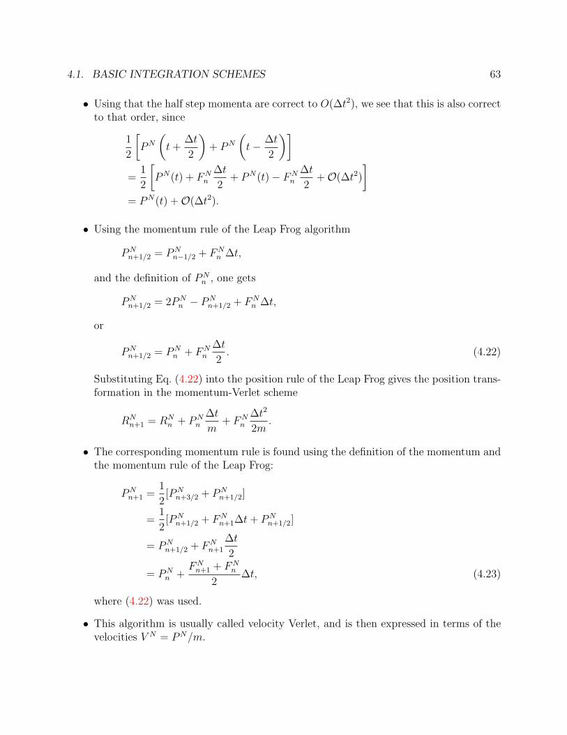
• The way the instability limit is approached is illustrated in figure 4.1, where ω and mare plotted as a function of ∆t.

• We see that while the renormalized frequency remains finite up to the limit ∆t = 2,the renormalized mass goes to infinity.

• This divergence shows that the pseudo Hamiltonian is not bounded.

• Only a bounded pseudo-Hamiltonian guarantees a stable algorithm.

• So an instability for large time steps arises even for the simple case of an harmonicoscillator

• The instability arises from an unbounded, diverging pseudo-Hamiltonian.

• Why could the pseudo-Hamiltonian diverge in the first place?

• Consider equation (4.38) again, which gives the pseudo-Hamiltonian as a power seriesin ∆t.

• Generally, power series converge only if ∆t < ∆t∗, where ∆t∗ is the radius of conver-gence.

4.5. MORE ACCURATE SPLITTING SCHEMES 79

0

0.5

1

1.5

2

2.5

3

0 0.5 1 1.5 2

reno

rmal

ized

quan

titie

s

dt

frequencymass

Figure 4.1: The way the instability limit is approached when using the Verlet splittingscheme on the harmonic oscillator. Plotted are the renormalized frequency ω and mass mas a function of ∆t. The unnormalized values were 1.

• For the harmonic oscillator, the radius of convergence was clearly ∆t∗ = 2.

• Also for general system, one expects a radius of convergence, i.e., a time step be-yond which the pseudo-Hamiltonian becomes unbounded and the simulation becomesunstable.

4.5 More accurate splitting schemes

• Higher order schemes give better accuracy, but at the price of performing more forcecomputations.

• Higher order schemes are very important in contexts such as astrophysics, where ac-curate trajectories matter.

• For MD, depending on the level of accuracy required, higher order schemes can alsobe advantageous.

• Higher order schemes may be devised by

– taking time points which are not evenly spaced,


– incorporating leading order correction terms in the pseudo-Hamiltonian

– incorporating more time points,

– or a combination of the above.

All but the first option lead to more force computations per unit of physical time,which decreases the efficiency.

• We will restrict ourselves to symmetric splitting schemes, to ensure time-reversibility.

• To facilitate many of the derivations, we restate the symmetrized BCH formula ofequation (4.34)

eXeY eX = e2X+Y− 16[X,[X,Y ]]+ 1

6[Y,[Y,X]]+fifth repeated X, Y commutators. (4.42)

4.5.1 Optimized schemes

• Given the same Hamiltonian split-up

H = K + U,

L = LK + LU ,

let us now explore a five-fold split up

eL∆t ≈ eηLU∆teLK∆t/2e(1−2η)LU∆teLK∆t/2eηLU∆t. (4.43)

• Note that this is a case of uneven time-intervals.

• Work out the inner three exponentials using equation (4.42)

eηLU∆teLK∆t/2e(1−2η)LU∆teLK∆t/2eηLU∆t

= eηLU∆teLK∆t+(1−2η)LU∆t− (1−2η)∆t3

24[LK ,[LK ,LU ]]+

(1−2η)2∆t3

12[LU ,[LU ,LK ]]+O(∆t5)eηLU∆t

= exp

{LK∆t + LU∆t− (1− 2η)∆t3

24[LK , [LK ,LU ]] +

(1− 2η)2∆t3

12[LU , [LU ,LK ]]

− η2∆t3

6[LU , [LU ,LK ]] +

η∆t3

6[LK + (1− 2η)LU , [LK ,LU ]] +O(∆t5)

}

= eLH∆t+∆t3

„6η−124

[LK ,[LK ,LU ]]+ 1−6η+6η2

12[LU ,[LU ,LK ]]

«+O(∆t5)

= eLH∆t+∆t3(ν1[LK ,[LK ,LU ]]+ν2[LU ,[LU ,LK ]])+O(∆t5)


where

ν1 =6η − 1

24

ν2 =1− 6η + 6η2

12

• If both ν1 and ν2 were zero, this would give a fourth order scheme.However, this is not possible here: we have one parameter and two prefactors to set tozero.

• Alternatively, one could make the error “as small as possible”, e.g. by minimizingν2

1 + ν22 . This gives

η = 0.1931833275037836 . . . (4.44)

• The scheme in equation (4.43) that uses this value of η is called the Higher-orderOptimized Advanced scheme of second order, or HOA2 for short.

• In general, optimized schemes are based on minimizing the formal error, but this cannotguarantee that the actual error is small: Numerical tests are necessary.

• The HOA2 scheme requires two force computations:

eηLU∆t︸︷︷︸from previous step

eLK∆t/2 e(1−2η)LU∆t︸︷︷︸1st force computation

eLK∆t/2 eηLU∆t︸︷︷︸2nd force computation,

(4.45)

whereas the Verlet scheme requires just one.

• Thus, to compare accuracies at fixed numerical cost, the time step should be takentwice as large in the HOA2 scheme as in the Verlet scheme.

• The HOA2 scheme was tested on a model of water (TIP4P) [Van Zon, Omelyan andSchofield, J. Chem. Phys 128, 136102 (2008)], with the following results:

– As long as it is stable, the HOA2 scheme leads to smaller fluctuations in the totalenergy than the Verlet scheme at the same computational cost.

– In the water simulation, the HOA2 scheme becomes unstable for smaller timesteps than the Verlet scheme.

– The superior stability of the Verlet scheme means that it is the method of choicefor quick and dirty simulations of water with an accuracy less than approximately1.5% (as measured by the energy fluctuations).


– For more accurate simulations, the HOA2 is more efficient, by about 50%, untilthe HOA2 scheme becomes unstable.

• The higher instability of HOA2 at large time steps, is due to the uneven time-stepsthan are taken.

• The average time step determines the computational cost, but the largest of the timesteps determines the stability.

• Using uneven time steps instead of even time steps (at fixed computational cost) there-fore increases some of the time intervals and decreases other.

• ⇒ uneven time steps become unstable for smaller time steps than even time stepvariants.

4.5.2 Higher order schemes from more elaborate splittings

• While using the HOA2 scheme is beneficial, this could only be known after numericaltests.

• True higher-order schemes are a bit better in that respect: one knows that at least forsmall enough ∆t, they are more efficient.

• The simplest way to get a higher order scheme is to concatenate lower order schemes.

• To understand this, note that if we have a k-th order scheme Sk(∆t) approximatingS(∆t) = eL∆ up to O(∆tk+1), i.e., if

Sk(∆t) = S(∆t) + ∆tk+1δS +O(∆tk+3)

then

Sk(∆s)Sk(∆t− 2∆s)Sk(∆s) (4.46)

= S(∆t) +[2∆sk+1 + (∆t− 2∆s)k+1

]δS +O(∆tk+3) (4.47)

The leading order term can be eliminated by choosing

2∆sk+1 = −(∆t− 2∆s)k+1, (4.48)

which, if k is even, can be solved and gives

∆s =∆t

2− 21/(k+1). (4.49)


• When Sk = S2 is given by the second Verlet scheme, the corresponding fourth orderscheme becomes

eL∆t ≈ eLU∆s/2eLK∆seLU∆s/2eLU (∆t/2−∆s)eLK(∆t−2∆s)eLU (∆t/2−∆s)eLU∆s/2eLK∆seLU∆s/2

= eLU∆s/2eLK∆seLU (∆t−∆s)/2eLK(∆t−2∆s)eLU (∆t−∆s)/2eLK∆seLU∆s/2 (4.50)

This is called the fourth order Forest-Ruth integration scheme (FR4). Note that it hasseven parts and requires three force evaluations per time step.

• Note that ∆s > ∆t/2, so that ∆t− 2∆s < 0.

• It therefore requires to take a negative time step:This tends to lead to instabilities.

• One can prove that order k splitting schemes using a two-operator split up (such asLU and LK) must have at least one negative time step if k > 2.

• The negative steps thus seem unavoidable.

• One can minimize these however, by allowing more general splitting schemes than thoseconstructed from equation (4.46), i.e., using the general form in equation (4.32).

• This gives more parameters, allowing one to combine this with the higher-order naturewith optimization, i.e. minimizing the leading error terms (cf. the HOA2 scheme).

• A good fourth order scheme of this type is called EFRL4 (Extended Forest-Ruth-likeFourth order scheme) and looks like this:

eL∆t = eLU ξ∆teLK( 12−λ)∆teLUχ∆teLKλ∆teLU (1−2χ−2ξ)∆teLKλ∆teLUχ∆teLK( 1

2−λ)∆teLU ξ∆t

(4.51)

+O(∆t5),

where

ξ = 0.3281827559886160

λ = 0.6563655119772320

χ = −0.09372690852966102

Even though this requires four force evaluations for each time step, it is more efficientthan the FR4 scheme due to a much smaller leading order error.


4.5.3 Higher order schemes using gradients

• Gradients are, in this context, derivatives and higher-order derivatives of the potential.

• Using gradients as auxiliary Hamiltonians, one can reduce the order of a scheme

• The simplest can be derived by considering once more the five-fold splitting scheme,before optimization:

eηLU∆teLK∆t/2e(1−2η)LU∆teLK∆t/2eηLU∆t = eLH∆t+∆t3(ν1[LK ,[LK ,LU ]]+ν2[LU ,[LU ,LK ]])+O(∆t5)

= eLH∆t+∆t3(ν1L{{U,K},K}+ν2L{{K,U},U})+O(∆t5)

where

ν1 =6η − 1

24

ν2 =1− 6η + 6η2

12

and let K and U be of the usual form such that (cf. equations (4.35) and (4.36))

{{K, U}, U} =∂U

∂RN· ∂2K

∂PN∂PN· ∂U

∂RN=

1

m

∣∣∣∣ ∂U

∂RN

∣∣∣∣2 =1

m|FN |2

{{U,K}, K} =∂K

∂PN· ∂2U

∂RN∂RN· ∂K

∂PN=

1

m2PN · ∂2U

∂RN∂RN· PN .

• The former depends only on RN , but the latter is more complicated and depends onboth RN and PN .

• We can eliminate the more complicated term by setting ν1 = 0 ⇒ η = 1/6, leaving uswith

e16LU∆te

12LK∆te

23LU∆te

12LK∆te

16LU∆t = e

LH∆t+∆t3 172m

L|FN |2+O(∆t5)

= e

»LK+L

U+ ∆t272m |FN |2

–∆t+O(∆t5)

• This equation holds for any form of U !

• Thus we may substitute for U the expression

U = U − ∆t2

72m

∣∣FN∣∣2 , (4.52)


giving

e16LU∆te

12LK∆te

23LU∆te

12LK∆te

16LU∆t = e

»LK+L

U+ ∆t272m |FN |2

–∆t+O(∆t5)

= e[LK+LU ]∆t+O(∆t5) = eLH∆t+O(∆t5)

A fourth order integration scheme!

• Note that no negative time steps were needed.

• The scheme in the current form uses an effective potential U , which differs from the

real potential U by an additional term δU = −∆t2

72m

∣∣FN∣∣2 of order O(∆t2). To leading

order, this term commutes with all factors, so one may also write

eLH∆t+O(∆t5) = e16LU∆te

12LK∆te

23LU∆t+δU∆te

12LK∆te

16LU∆t

= e16LU∆te

12LK∆te

23[LU+ 3

2δU ]∆te

12LK∆te

16LU∆t

= e16LU∆te

12LK∆te

23[L ˜U

]∆te12LK∆te

16LU∆t (4.53)

where the modified potential in the middle step is

˜U = U +3

2δU = U − ∆t2

48m

∣∣FN∣∣2 . (4.54)

• Scheme (4.53) is due to Suzuki.

• To summarize: by taking uneven intervals and incorporating the correction terms(using gradients of the potentials), we get a fourth order scheme which does not requirenegative partial steps and only needs two force evaluations per step.

• Note that to be able to use the modified potentials, the forces have to be well defined,i.e., any cut-off has to be smooth enough.

4.5.4 Multiple time-step algorithms

• Decompose the potential and the corresponding Liouville operator into two parts: onefor fast varying forces and the other for the slow varying forces:

U = Uf + Us (4.55)

• The fast motion could represent e.g. , intermolecular vibrations while the slowly varyingforces might be intermolecular forces.


• The simplest multiple time-step algorithm is then

e12LUs∆t

(e

12LUf

∆t/MeLK∆t/Me12LUf

∆t/M)M

e12LUs∆t = eL∆t+O(∆t3). (4.56)

• While this is of second order, like the Verlet scheme, the time step for the fast part ofthe motion if M times smaller than that of the slow motion.

Date post:	27-Mar-2020
Category:	Documents
Upload:	others
View:	2 times
Download:	0 times

4 Molecular dynamics - University of Toronto · 2011-05-03 · 4 Molecular dynamics 4.1 Basic...

Documents