ME 349, Engineering Analysis, Alexey Volkov 1 4. Numerical analysis II 1. Numerical differentiation 2. Numerical integration 3. Ordinary differential equations (ODEs). First‐order ODEs 4. Numerical methods for initial value problems (individual ODEs) 5. Second‐ and higher order ODEs. Systems of ODEs 6. Numerical methods for initial value problems (systems of ODEs) 7. Numerical solution of IVPs with build‐in MATLAB solvers 8. Summary Text A. Gilat, MATLAB: An Introduction with Applications, 4th ed., Wiley
Transcript
ME 349, Engineering Analysis, Alexey Volkov 1
4. Numerical analysis II1. Numerical differentiation2. Numerical integration3. Ordinary differential equations (ODEs). First‐order ODEs4. Numerical methods for initial value problems (individual ODEs)5. Second‐ and higher order ODEs. Systems of ODEs6. Numerical methods for initial value problems (systems of ODEs)7. Numerical solution of IVPs with build‐in MATLAB solvers8. Summary
Text
A. Gilat, MATLAB: An Introduction with Applications, 4th ed., Wiley
ME 349, Engineering Analysis, Alexey Volkov 2
4.1. Numerical differentiation Formulation of the problem General approach to numerical differentiation Finite‐different approximation of the first‐order derivatives Finite‐different approximation of the second‐order derivatives Problems
ME 349, Engineering Analysis, Alexey Volkov 3
4.1. Numerical differentiationFormulation of the problem and general approach to numerical differentiation
Let's assume that a functional dependence between two variables and is given in thetabulated form: We know , for discrete values of the argument , 1, … , . Ourgoal is to find numerically (i.e. approximately) the derivative ′
The general approach to the numerical differentiation involves only two steps: We need to find an interpolation polynomial for the given data points
⋯ Then ′ can be find approximately as a derivative of the interpolation polynomial
2 3 ⋯ 1
Interpolation function
Interpolation in Interpolation interval ,
(4.1.1)
ME 349, Engineering Analysis, Alexey Volkov 4
4.1. Numerical differentiationNodal values of derivatives at a uniform mesh
In many applications, e.g. for numerical solution of differential equations, we are interestedin finding derivatives
For data points given on amesh with equal spacing ∆ when ∆ 1 . Only in data points, i.e. finding only nodal values of derivatives .
In this case, the explicit solution of the interpolation problem (finding coefficients of theinterpolation polynomial in Eq. (4.1.1)) is not necessary.
One can obtain very simple and compact formulas for nodal values in terms ofand ∆ . Such formulas are known as finite‐difference formulas (approximations, equations).
∆ ∆
?
∆
ME 349, Engineering Analysis, Alexey Volkov 5
4.1. Numerical differentiationTaylor series on a uniform mesh
One can use the Taylor series in order to find derivatives on a mesh with equal spacing
12
16 …
Let’s use this equation with and different , , etc.
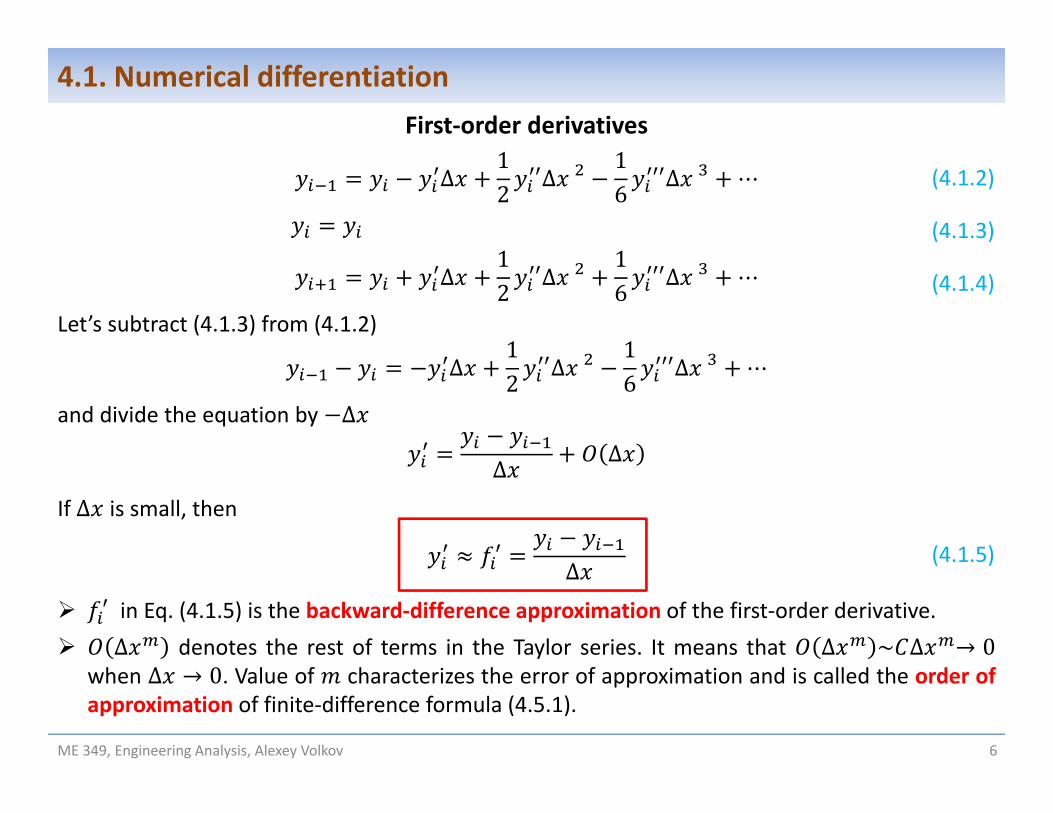
Δ in Eq. (4.1.5) is the backward‐difference approximation of the first‐order derivative. ∆ denotes the rest of terms in the Taylor series. It means that ∆ ~ ∆ → 0
when ∆ → 0. Value of characterizes the error of approximation and is called the order ofapproximation of finite‐difference formula (4.5.1).
(4.1.2)
(4.1.3)
(4.1.4)
(4.1.5)
ME 349, Engineering Analysis, Alexey Volkov 7
4.1. Numerical differentiation
∆12 ∆
16 ∆ ⋯
∆12 ∆
16 ∆ ⋯
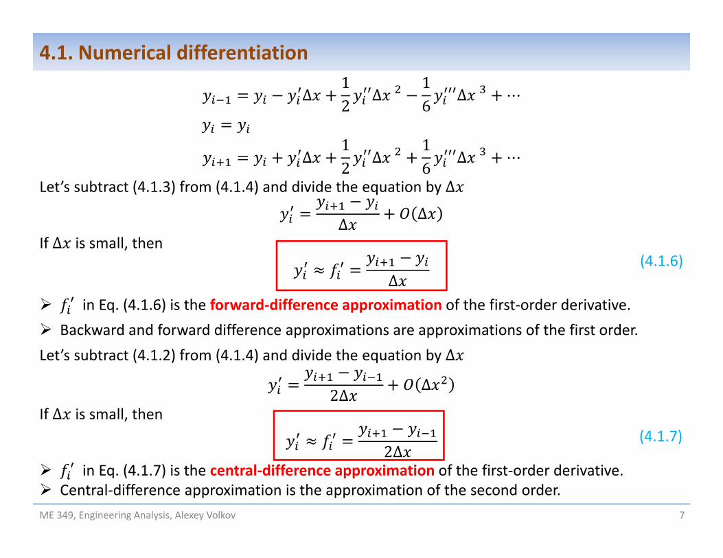
Let’s subtract (4.1.3) from (4.1.4) and divide the equation by ∆
Δ ∆
If ∆ is small, then
Δ in Eq. (4.1.6) is the forward‐difference approximation of the first‐order derivative. Backward and forward difference approximations are approximations of the first order.Let’s subtract (4.1.2) from (4.1.4) and divide the equation by ∆
2Δ ∆
If ∆ is small, then
2Δ in Eq. (4.1.7) is the central‐difference approximation of the first‐order derivative. Central‐difference approximation is the approximation of the second order.
(4.1.6)
(4.1.7)
ME 349, Engineering Analysis, Alexey Volkov 8
4.1. Numerical differentiationGeometrical interpretation of finite difference formulas
The same derivative can be approximated with different finite‐difference formulas. If is smooth, the higher the order of approximation, the more accurate the formula.
∆ ∆Δ
Δ
2Δ
∆ ∆
∆ ∆
tan
Finite‐difference formulas approximate the derivative with the slope of corresponding chord connecting nodal values of
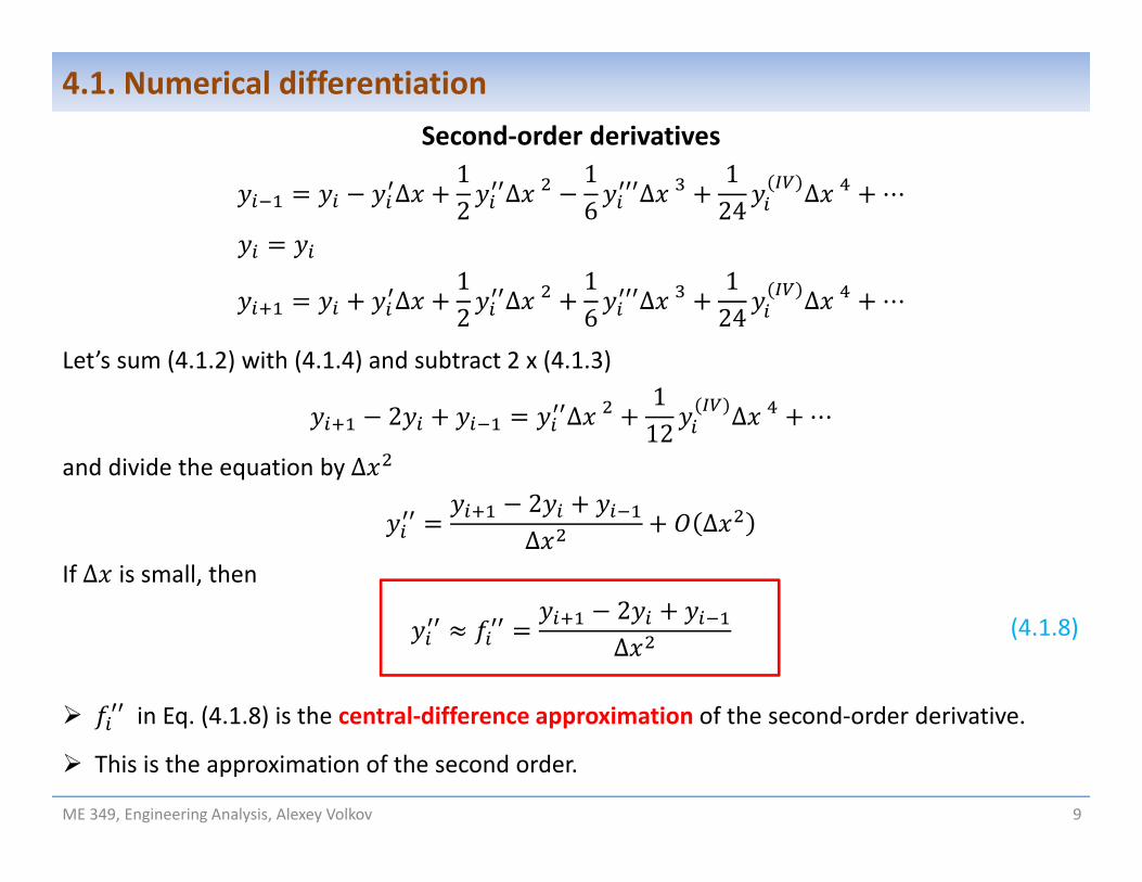
Let’s sum (4.1.2) with (4.1.4) and subtract 2 x (4.1.3)
2 ∆ 112 ∆ ⋯
and divide the equation by∆2∆ ∆
If ∆ is small, then2∆
in Eq. (4.1.8) is the central‐difference approximation of the second‐order derivative.
This is the approximation of the second order.
(4.1.8)
ME 349, Engineering Analysis, Alexey Volkov 10
4.1. Numerical differentiationSummary on numerical differentiating with MATLAB
Central finite differences of the second order of approximation for function :
2Δ ,2∆
Δ Δ2Δ , ′′
Δ 2 Δ∆
Example:
x = 1.0;dx = 0.01;dydx = ( Fun ( x + dx ) ‐ Fun ( x ‐ dx ) ) / ( 2.0 * dx );d2ydx2 = ( Fun ( x + dx ) ‐ 2.0 * Fun ( x ) + Fun ( x ‐ dx ) ) / dx^2;
function [ y ] = Fun ( x )
y = x^2;
end
Problem 4.1.1: Calculate numerically the first‐order derivative of the functionsin log 1
at point 2 with ∆ 0.1 and ∆ 0.01 using backward and central finite differences andcompare then with accurate values by calculating the relative numerical error:
With decreasing ∆ in 10 times, err_b decreases in 10 time, while err_c decreases in 100times!
ME 349, Engineering Analysis, Alexey Volkov 11
4.1. Numerical differentiation
ME 349, Engineering Analysis, Alexey Volkov 12
4.1. Numerical differentiationProblem 4.1.2: Calculation of velocity and acceleration in points of a trajectory given in a tabulated from
where 1 ∆ and ∆ is the time step. Our goal is to find numerically and plot the body velocity andforce affecting the body at times using central finite differences.function [] = VelocityAndAcceleration ( Dt, X, Y, N )
File Problem_4_1_2:t = [ 0 : 0.1 : 2 ];X = sin ( t );Y = 2 * cos ( t ) ‐ 1;VelocityAndAcceleration ( 0.1, X, Y, 21 );
Let's solve the problemassuming that trajectory is given by equations
sin2 cos 1
Trajectory
Acceleration
Velocity
ME 349, Engineering Analysis, Alexey Volkov 13
4.2. Numerical Integration Formulation of the problem Elementary approach for the numerical integration Rectangle rule Trapezoidal rule Numerical integration in the MATLAB
Reading assignmentGilat 9.3
ME 349, Engineering Analysis, Alexey Volkov 14
4.2. Numerical integrationFormulation of the problem
Let’s assume that we want to find the value of definite integral of the integrand in theinterval ,
The integrand can be given in either the explicit function form (e.g.,exp sin ) or tabulated form, i.e. for discrete , 1,… , .
In many practical cases, we cannot evaluate the integral algebraically, i.e. to findantiderivative , such that ′ , .Example:
Our goal is to find the value of the integral in Eq. (4.2.1) numerically (approximately), i.e.perform numerical integration (find numerical quadrature) of the integrand in theinterval , .
Quadrature is a historical mathematical term which means determining area. The rules of the numerical integration are called quadrature rules.
(4.2.1)
The geometrical meaning of an intervalThe integral is the signed area of the shape bounded by the plot of integrand and axis
Major property of definite integral: Additivity on intervals
ME 349, Engineering Analysis, Alexey Volkov 15
4.2. Numerical integration
(4.2.2)
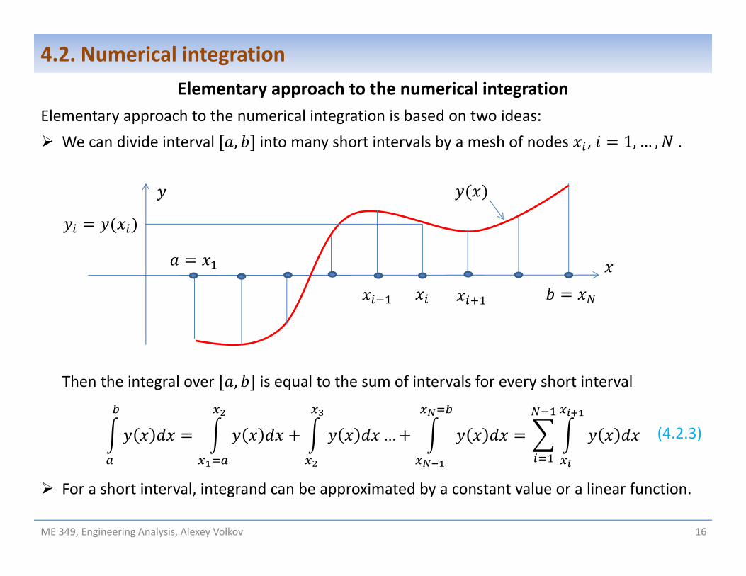
Elementary approach to the numerical integrationElementary approach to the numerical integration is based on two ideas: We can divide interval , into many short intervals by a mesh of nodes , 1,… , .
Then the integral over , is equal to the sum of intervals for every short interval
…
For a short interval, integrand can be approximated by a constant value or a linear function.
ME 349, Engineering Analysis, Alexey Volkov 16
4.2. Numerical integration
(4.2.3)
Rectange (mid‐point) ruleAt every mesh interval , the value of the signed area is estimated as an area of acorresponding rectangle.
ME 349, Engineering Analysis, Alexey Volkov 17
4.2. Numerical integration
(4.2.4) / : Rectange rule
/
/12
For a mesh with equal spacing ∆ , / ∆ /2:
∆ ∆ /2
: Rectange rulefor a mesh withequal spacing(4.2.5)
Signed area of the rectangle is equal to
/
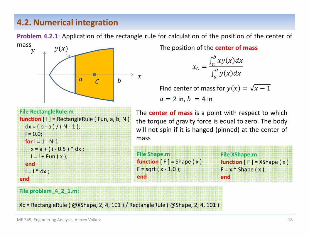
Problem 4.2.1: Application of the rectangle rule for calculation of the position of the center ofmass
ME 349, Engineering Analysis, Alexey Volkov 18
4.2. Numerical integration
File RectangleRule.mfunction [ I ] = RectangleRule ( Fun, a, b, N )dx = ( b ‐ a ) / ( N ‐ 1 );I = 0.0;for i = 1 : N‐1x = a + ( i ‐ 0.5 ) * dx ;I = I + Fun ( x );
File Shape.mfunction [ F ] = Shape ( x ) F = sqrt ( x ‐ 1.0 );end
The position of the center of mass
Find center of mass for 12 in, 4in
File XShape.mfunction [ F ] = XShape ( x ) F = x * Shape ( x );end
The center of mass is a point with respect to whichthe torque of gravity force is equal to zero. The bodywill not spin if it is hanged (pinned) at the center ofmass
Trapezoidal ruleAt every mesh interval , the value of the signed area is estimated as a signed areaof a corresponding trapezium.
ME 349, Engineering Analysis, Alexey Volkov 19
4.2. Numerical integration
(4.2.6)12
: Trapezoidalrule
For a mesh with equal spacing ∆ :
∆2 ∆ 2 (4.2.7)
: Trapezoidalrule for amesh withequal spacing
Signed area of the trapezium is equal to12
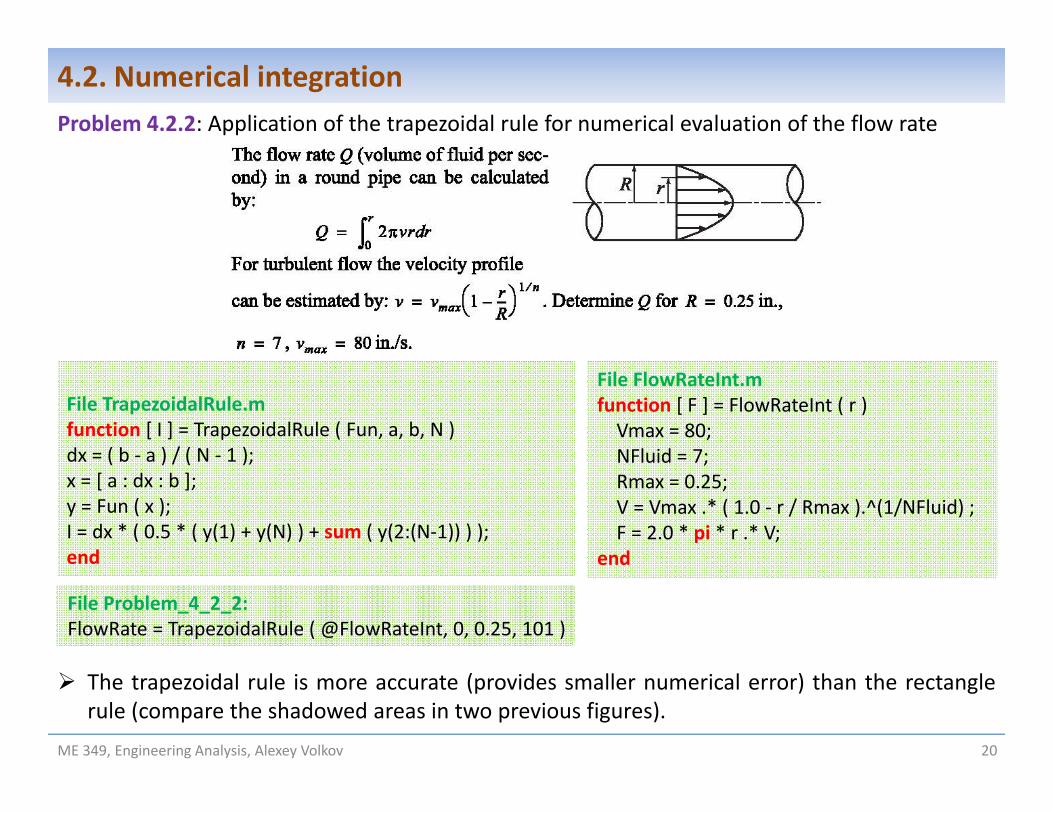
Problem 4.2.2: Application of the trapezoidal rule for numerical evaluation of the flow rate
The trapezoidal rule is more accurate (provides smaller numerical error) than the rectanglerule (compare the shadowed areas in two previous figures).
ME 349, Engineering Analysis, Alexey Volkov 20
4.2. Numerical integration
File TrapezoidalRule.mfunction [ I ] = TrapezoidalRule ( Fun, a, b, N )dx = ( b ‐ a ) / ( N ‐ 1 );x = [ a : dx : b ];y = Fun ( x );I = dx * ( 0.5 * ( y(1) + y(N) ) + sum ( y(2:(N‐1)) ) );end
File FlowRateInt.mfunction [ F ] = FlowRateInt ( r ) Vmax = 80;NFluid = 7;Rmax = 0.25;V = Vmax .* ( 1.0 ‐ r / Rmax ).^(1/NFluid) ;F = 2.0 * pi * r .* V;
end
Build‐in MATLAB functions for numerical integration
In order to calculate numerically the integrals of the form one can use thebuild‐in quad function.
It implements adaptive integration algorithms, when the mesh spacing ∆varies in the course of integration in order to ensure that error is within given tolerance.
Syntax: I = quad ( @Fun, a, b, Tol )
Fun is the (user‐defined) function that implements calculation of the integrand
a and b are the left‐ and right‐hand side limits of the integration interval , .
Tol in the optional tolerance parameter for the adaptive integration method. DefaultTol=1.0e‐6.
This is important: In order to be used in the quad function, the integrand should be writtenfor an input argument that is a vector of mesh values and the output argument that is avector of the mesh values of . We must use the elementwise operations.
ME 349, Engineering Analysis, Alexey Volkov 21
4.2. Numerical integration
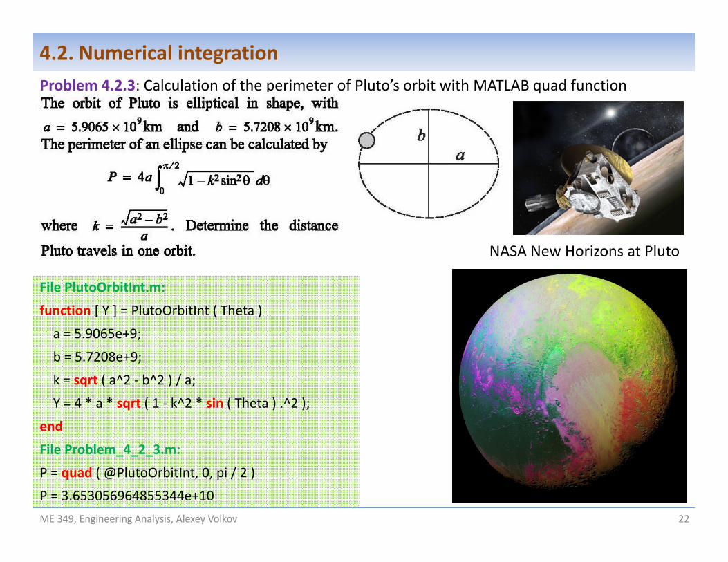
Problem 4.2.3: Calculation of the perimeter of Pluto’s orbit with MATLAB quad function
File PlutoOrbitInt.m:
function [ Y ] = PlutoOrbitInt ( Theta )
a = 5.9065e+9;
b = 5.7208e+9;
k = sqrt ( a^2 ‐ b^2 ) / a;
Y = 4 * a * sqrt ( 1 ‐ k^2 * sin ( Theta ) .^2 );
end
File Problem_4_2_3.m:
P = quad ( @PlutoOrbitInt, 0, pi / 2 )
P = 3.653056964855344e+10ME 349, Engineering Analysis, Alexey Volkov 22
4.2. Numerical integration
NASA New Horizons at Pluto
Summary on numerical integration with build‐in MATLAB function quadThe MATLAB build‐in function quad allows one to find a definite integral:
I = quad ( @fun, a, b )
Example:, 2, 2
function [ y ] = fun ( x )y = x.^2;
endI = quad ( @fun, ‐2.0, 2.0 )
ME 349, Engineering Analysis, Alexey Volkov 23
4.2. Numerical integration
Name of a function ‐ Integrand
Integration limits
Element‐by‐element operations must be used !!!
ME 349, Engineering Analysis, Alexey Volkov 24
4.3. Ordinary differential equations (ODEs). First‐order ODEs A concept of an ordinary differential equation. Order of an ODE General and particular solution of an ODE Initial conditions. Initial value problem for a 1st order ODE Example: Radioactive decay
ME 349, Engineering Analysis, Alexey Volkov 25
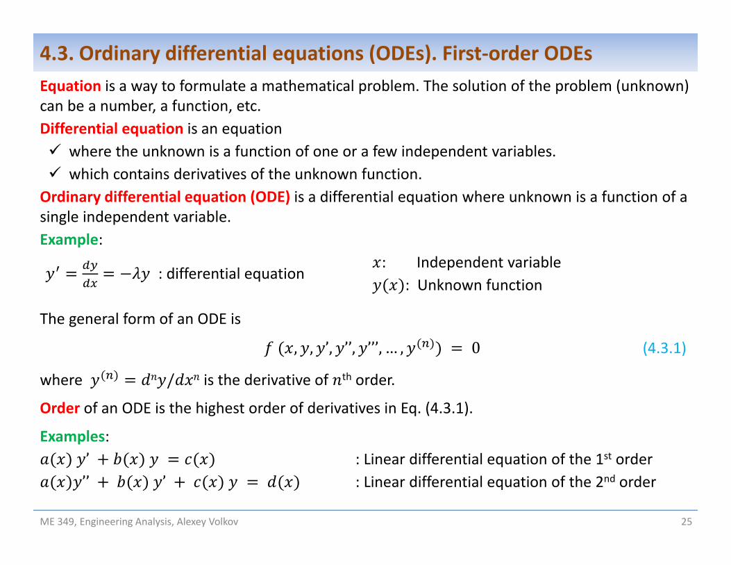
4.3. Ordinary differential equations (ODEs). First‐order ODEsEquation is a way to formulate a mathematical problem. The solution of the problem (unknown) can be a number, a function, etc.Differential equation is an equation where the unknown is a function of one or a few independent variables. which contains derivatives of the unknown function.Ordinary differential equation (ODE) is a differential equation where unknown is a function of a single independent variable.Example:
: Independent variable: Unknown function
The general form of an ODE is
, , ’, ’’, ’’’, … , 0 (4.3.1)
where / is the derivative of th order.
Order of an ODE is the highest order of derivatives in Eq. (4.3.1).
Examples: ’ : Linear differential equation of the 1st order’’ ’ : Linear differential equation of the 2nd order
: differential equation
ME 349, Engineering Analysis, Alexey Volkov 26
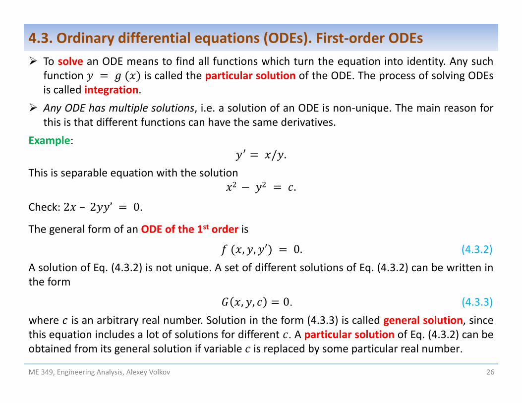
4.3. Ordinary differential equations (ODEs). First‐order ODEs To solve an ODE means to find all functions which turn the equation into identity. Any such
function is called the particular solution of the ODE. The process of solving ODEsis called integration.
Any ODE has multiple solutions, i.e. a solution of an ODE is non‐unique. The main reason forthis is that different functions can have the same derivatives.
Example: / .
This is separable equation with the solution 2 2 .
Check: 2 – 2 ’ 0.
The general form of an ODE of the 1st order is
, , ′ 0. (4.3.2)A solution of Eq. (4.3.2) is not unique. A set of different solutions of Eq. (4.3.2) can be written inthe form
, , 0. (4.3.3)where is an arbitrary real number. Solution in the form (4.3.3) is called general solution, sincethis equation includes a lot of solutions for different . A particular solution of Eq. (4.3.2) can beobtained from its general solution if variable c is replaced by some particular real number.
ME 349, Engineering Analysis, Alexey Volkov 27
4.3. Ordinary differential equations (ODEs). First‐order ODEsInitial value problem
In many engineering applications we are not interested in the general solution of an ODE, butwe are interested in the particular solution that satisfies some additional condition(s). For the 1storder ODE of in the explicit form (resolved with respect to the derivative)
,such conditions can be formulated as a requirement that at some given point 0thesolution is equal to the prescribed value y0, i.e.
or
Eq. (4.3.5) is called the initial condition for Eq. (4.3.4).A problem given by (4.3.4) and (4.3.5) is called the initial value (or Cauchy) problem (IVP).Example:ODE: d / /Initial condition: 1 2General solution: ⟹ c
2 2 Solution of the IVP: 1 2 3 and 3 If we want to check that some formula is a solution of the IVP, we need to check that
This formula turns the ODE into identity. This formula satisfies the initial condition.
4.3. Ordinary differential equations (ODEs). First‐order ODEsProblem 4.3.1: Radioactive decay of a radioactive substancePhysical law: Radioactive decay rate (number of nuclei exhibiting decay per unit time) isproportional to the current number of nuclei.
, number of nuclei at time
0 0 , Initial conditions: number of nuclei at initial time 0′ / 0, decay rate with the negative sign
1st order ODE / General solution: 0exp Exponential decayParticular solution: 10 exp Check: ’ 0exp
Half‐life τ is the time when a half of initial nuclei decayed
0/2 0exp
ln2/
t
N
N0
File RadioactiveDecay.mfunction Y = RadioactiveDecay ( X, Lam, A, YA )Y = YA * exp ( ‐ Lam * ( X ‐ A ) );
end
ME 349, Engineering Analysis, Alexey Volkov 29
4.4. Numerical methods for initial value problems (individual ODEs) Basic concepts of the numerical methods for IVPs The Euler method Implementation of the IVP solver in MATLAB Truncation errors and order of approximation The Runge‐Kutta methods Numerical solution of IVPs in the MATLAB
Reading assignmentGilat 9.4
ME 349, Engineering Analysis, Alexey Volkov 30
4.4. Numerical methods for initial value problems (individual ODEs)Let’s consider a 1st ODE in the explicit form
′ ,
Assume that we are not able to solve this equation algebraically, i.e. we cannot find a function, or , , 0 that represents the general solution of this equation.
On the other hand, virtually any ODE can be solved numerically with the help of a computerthat performs basic algebraic operations ( , , ) with integer and real numbers.
In order to solve an IVP numerically, we need to develop an algorithm that allows us to calculateapproximate values of the unknown function in this equation with a finite number of algebraicoperations. Such algorithms for solving different mathematical problems are called numericalmethods or numerical schemes.
Basic concepts of the numerical methods for IVPs
1. Numerically we can look only for a particular solution of an ODE or a system of ODEs, i.e. wecan solve only initial or boundary value problems. For the first‐order ODE we can solvenumerically only the Cauchy problem with the initial condition
, , , (4.1.1)
ME 349, Engineering Analysis, Alexey Volkov 31
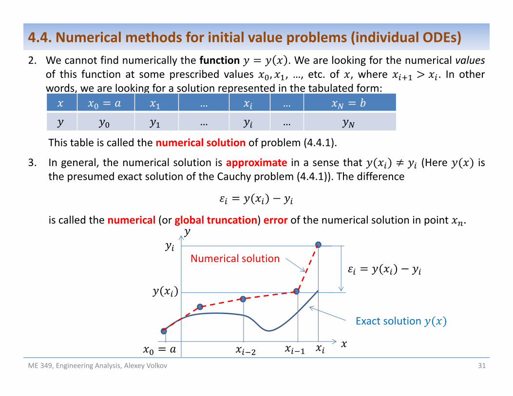
4.4. Numerical methods for initial value problems (individual ODEs)2. We cannot find numerically the function . We are looking for the numerical values
of this function at some prescribed values , , …, etc. of , where . In otherwords, we are looking for a solution represented in the tabulated form:
This table is called the numerical solution of problem (4.4.1).
3. In general, the numerical solution is approximate in a sense that (Here isthe presumed exact solution of the Cauchy problem (4.4.1)). The difference
is called the numerical (or global truncation) error of the numerical solution in point .
… …
… …
Exact solution
Numerical solution
32
4.4. Numerical methods for initial value problems (individual ODEs)The Euler method
Let's develop the simplest numerical method to solve an IVP
, , , .1. Let's introduce a mesh of nodes with the spacing ∆ : ∆ .2. Let's approximate derivative in the ODE in node with the forward finite difference
, or ∆ , .
3. We start from the point and given by the initial condition and apply Eq.(4.4.2) in order to find :
∆ , , ∆3. Now we can repeat step 2 recursively
∆ , , ∆
until 1 ∆ .
(4.4.2)
The numerical method given by Eqs. (4.4.3)is called the (explicit) Euler method.
Graphically, the numerical algorithm of theEuler method can be shown as follows:
∆ ,Tangent
tan ,
(4.4.1)
(4.4.3)
ME 349, Engineering Analysis, Alexey Volkov
33
4.4. Numerical methods for initial value problems (individual ODEs) The whole process of numerical solution looks like a sequence of individual integration steps
Value ∆ (increment of the independent variable during one integration step) iscalled the integration step size. In our case ∆ ∆ , but in general the integrationstep does not need to be constant at every .
Numerical solution is the solution of the finite difference equation and depends on thenumerical parameter(s), the integration step size, which is absent in the original IVP.
The integration step size controls the numerical error , where is theaccurate solution of the problem given by Eq. (4.4.1).
Our obvious goal is to chose such numerical parameter that allows us to obtain a numericalsolution that approximates the accurate solution of the problem with sufficient accuracy.
ME 349, Engineering Analysis, Alexey Volkov
∆
Integration step : →
Initialcondition
tan ,
34
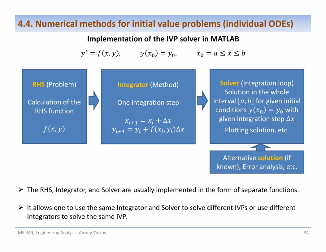
4.4. Numerical methods for initial value problems (individual ODEs)Implementation of the IVP solver in MATLAB
, , ,
ME 349, Engineering Analysis, Alexey Volkov
RHS (Problem)
Calculation of the RHS function
,
Integrator (Method)
One integration step
∆, ∆
Solver (Integration loop)Solution in the whole
interval , for given initial conditions with given integration step ∆Plotting solution, etc.
Alternative solution (if known), Error analysis, etc.
The RHS, Integrator, and Solver are usually implemented in the form of separate functions.
It allows one to use the same Integrator and Solver to solve different IVPs or use different Integrators to solve the same IVP.
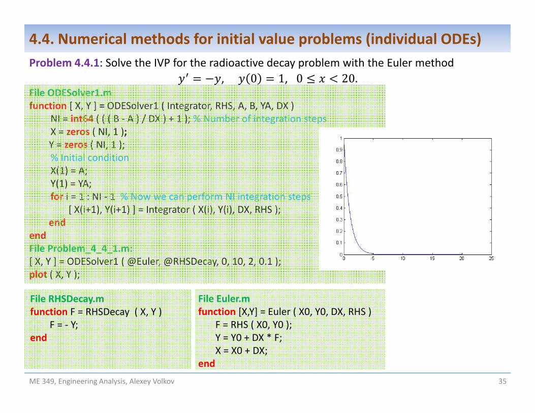
Problem 4.4.1: Solve the IVP for the radioactive decay problem with the Euler method , 0 1, 0 20.
File ODESolver1.mfunction [ X, Y ] = ODESolver1 ( Integrator, RHS, A, B, YA, DX )
NI = int64 ( ( ( B ‐ A ) / DX ) + 1 ); % Number of integration stepsX = zeros ( NI, 1 ); Y = zeros ( NI, 1 ); % Initial conditionX(1) = A; Y(1) = YA; for i = 1 : NI ‐ 1 % Now we can perform NI integration steps
end figure ( 1 ); % First figure is the solutionplot ( X, Y, 'r‐', X, Yacc, 'g‐‐' ) ; title ('Numerical (red) and accurate (green) solutions');figure ( 2 ); % Second figure is the numerical errorloglog ( X, E ); title ('Relative error of the numerical solution');
4.4. Numerical methods for initial value problems (individual ODEs)
ME 349, Engineering Analysis, Alexey Volkov
File SolDecay.mfunction Y = SolDecay ( X, A, YA )
Y = YA * exp ( A ‐ X );end
Relative numerical error
IVP: , 0 1, 0 20. Accurate solution: exp .
Numerical solutions Relative numerical error | / | vs.
Conclusions:1. The smaller the integration step, the better the accuracy of the numerical solution.2. | |/ increases with , so that eventually the error becomes unacceptably large.3. For the Euler method, the numerical error at given is proportional to ∆ .4. There is a some “critical value” ∆ . if ∆ ∆ , then the numerical solution has no
physical sense and useless.
37
4.4. Numerical methods for initial value problems (individual ODEs)
ME 349, Engineering Analysis, Alexey Volkov
ME 349, Engineering Analysis, Alexey Volkov 38
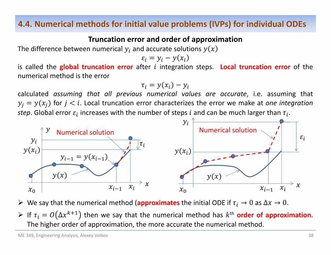
Truncation error and order of approximationThe difference between numerical and accurate solutions
is called the global truncation error after integration steps. Local truncation error of thenumerical method is the error
calculated assuming that all previous numerical values are accurate, i.e. assuming thatfor . Local truncation error characterizes the error we make at one integration
step. Global error increases with the number of steps and can be much larger than .
We say that the numerical method (approximates the initial ODE if → 0 as ∆ → 0. If ∆ then we say that the numerical method has th order of approximation.
The higher order of approximation, the more accurate the numerical method.
Numerical solution Numerical solution
4.4. Numerical methods for initial value problems (IVPs) for individual ODEs
The Euler method has the first order of approximation. Usually, it is insufficiently accurate tosolve practical problem.
The Runge‐Kutta methodsThe idea of the Runge‐Kutta methods is to use additional values of the RHS of the ODE at theinterval in order to increase the order of approximation and accuracy.1st order Euler method 2nd order Runge‐Kutta
The Runge‐Kutta method of the second order (RK2) (improved Euler method) can beformulated as follows: ∆ , ∆ 0.5∆ , 0.5 , ∆
It can be proved that RK2 method has the second order of approximation.
ME 349, Engineering Analysis, Alexey Volkov 39
(4.4.4)
∆ ,1 1
2
3
0.5∆
4.4. Numerical methods for initial value problems (IVPs) for individual ODEs
Implementation of RK2 in MATLAB:File RK2.mfunction [ X, Y ] = RK2 ( X0, Y0, DX, RHS )
Development of the RK methods of higher order requires complex algebra.
Popular Runge‐Kutta method of the 4th order (RK4) can be formulated as follows:
∆ , ∆ 0.5∆ , 0.5 ∆ 0.5∆ , 0.5 ∆ ∆ ,
16 2 2
∆
See MATLAB implementation of RK4 on the blackboard.ME 349, Engineering Analysis, Alexey Volkov 40
(4.4.5)
4.4. Numerical methods for initial value problems for individual ODEs
12
3
0.5∆
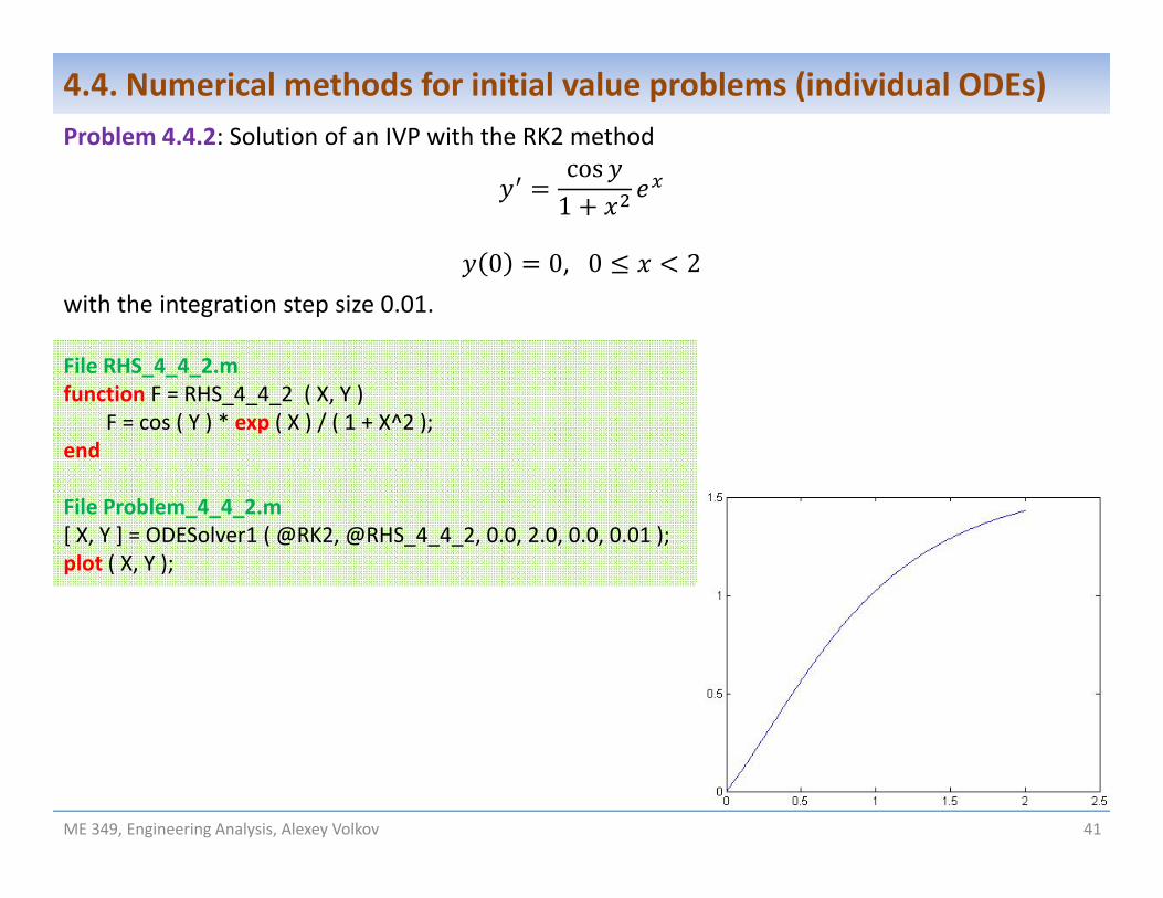
Problem 4.4.2: Solution of an IVP with the RK2 methodcos1
0 0, 0 2with the integration step size 0.01.
File RHS_4_4_2.mfunction F = RHS_4_4_2 ( X, Y )
F = cos ( Y ) * exp ( X ) / ( 1 + X^2 );end
File Problem_4_4_2.m[ X, Y ] = ODESolver1 ( @RK2, @RHS_4_4_2, 0.0, 2.0, 0.0, 0.01 );plot ( X, Y );
ME 349, Engineering Analysis, Alexey Volkov 41
4.4. Numerical methods for initial value problems (individual ODEs)
42
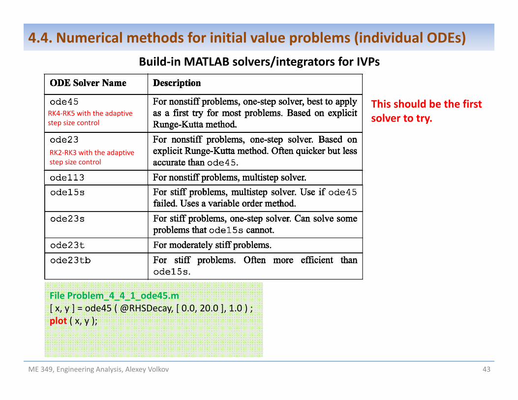
4.4. Numerical methods for initial value problems (individual ODEs)Build‐in MATLAB functions for numerical solutions of the IVP for first‐order ODEs
, , ,
MATLAB has a lot of build‐in solvers (integrators) for IVPs for first‐order ODEs that implementnumerical methods with the adaptive step size control, when the integration step size ischanged in the course of integration in order to ensure that the numerical error is within agiven tolerance.
These solvers implement different numerical methods, but have the same syntax.
Syntax: [ x, y ] = Solver ( @Fun, xspan, ya ) Solver is the name of the solver (see the next slide). Fun in the (user‐defined) function that implements calculation of the RHS , . xspan is 1D array that should contain at least two real values. The first and last elements
of xspan are used as limits of the integration interval , . ya is the initial condition for at . x and y are the column vectors with nodes values of and obtained as a result of
integration. Values of x depend on xspan (see Gilat's textbook, p. 306).
ME 349, Engineering Analysis, Alexey Volkov
Build‐in MATLAB solvers/integrators for IVPs
43
4.4. Numerical methods for initial value problems (individual ODEs)
ME 349, Engineering Analysis, Alexey Volkov
This should be the first solver to try.RK4‐RK5 with the adaptive
step size control
RK2‐RK3 with the adaptive step size control
File Problem_4_4_1_ode45.m[ x, y ] = ode45 ( @RHSDecay, [ 0.0, 20.0 ], 1.0 ) ;plot ( x, y );
Comparison of numerical accuracy of the RK2 with fixed integration step size and ode45 with adaptive step size control
44
4.4. Numerical methods for initial value problems (individual ODEs)
ME 349, Engineering Analysis, Alexey Volkov
RK2 with ∆ 0.01 ode45 with adaptive step size control
Relative numerical error in the "exponential decay problem" (slides 28, 37)
Adaptive step size control algorithm is not absolutely universal and sometimes leads tounsatisfactory results.
Constant integration step size often results in a linear increase of the numerical error. Theintegration step size appropriate for a particular problem can be chosen by means ofexperimentation (obtaining a series of numerical solutions with gradually decreasing ∆ ).
4.4. Numerical methods for initial value problems (individual ODEs)
ME 349, Engineering Analysis, Alexey Volkov
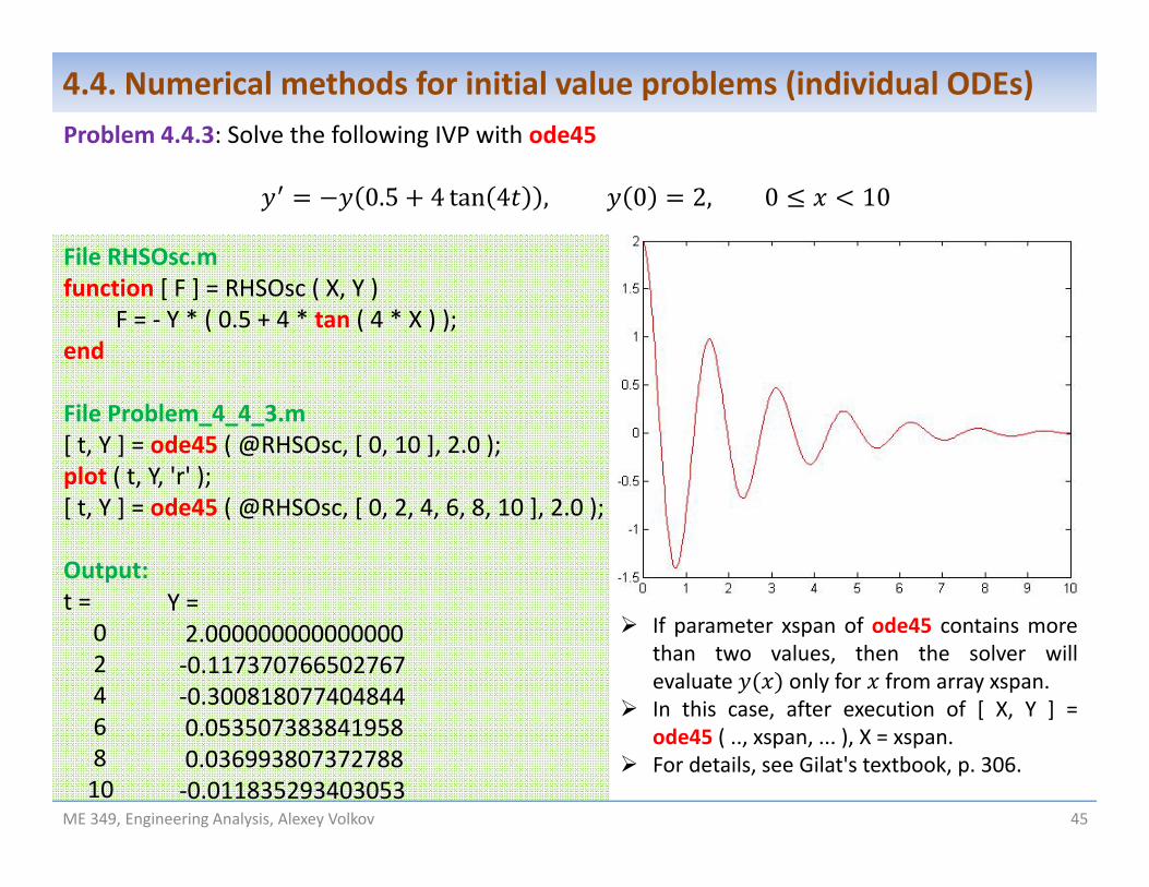
Y =2.000000000000000‐0.117370766502767‐0.3008180774048440.0535073838419580.036993807372788‐0.011835293403053
If parameter xspan of ode45 contains morethan two values, then the solver willevaluate only for from array xspan.
In this case, after execution of [ X, Y ] =ode45 ( .., xspan, ... ), X = xspan.
For details, see Gilat's textbook, p. 306.
Summary on numerical integration of ODEs with build‐in MATLAB function ode45The MATLAB build‐in function ode45 allows one to solve an initial value problem:
, , , .
[ x, y ] = ode45 ( @fun, [ a, b ], y0 )
Example:
sin , 1 1, 1 2
function [ f ] = fun ( x, y )f = sin ( x ) * y^2;
end[ x, y ] = ode45 ( @fun, [ 1.0, 2.0 ], ‐ 1.0 );plot ( x, y )
ME 349, Engineering Analysis, Alexey Volkov 46
4.4. Numerical methods for initial value problems (individual ODEs)
Name of a function ‐ RHS ,
Integration limits
Initial condition
Tables (1D arrays) of and
ME 349, Engineering Analysis, Alexey Volkov 47
4.5. Second‐ and higher order ODEs. Systems of ODEs Second order ODEs. Initial value problem (IVP) Example: Mass‐spring mechanical system Systems of ODEs. Fundamental systems Reduction of higher order ODEs in the normal form to a fundamental system of
first‐order ODEs. Matrix notation for fundamental systems
Reading assignmentGilat 9.4
ME 349, Engineering Analysis, Alexey Volkov 48
Second‐order ODE. Initial value problemGeneral form of the 2nd order ODE
(4.5.1)We will consider only equations in the explicit form, resolved with respect to the highestderivative
(4.5.2)The general solution of Eq. (4.5.2) depends on two constants and and can be written as:
(4.5.3)Example:
Any particular choice of constants and gives a particular solution of Eq. (4.5.2).One possible way to determine and is to specify the initial conditions
(4.5.4)
The problem given by Eqs. (4.5.2) and (4.5.4) is called the initial value (or Cauchy) problem (IVP)for the 2nd order ODE.
In mechanics, if is time and is coordinate, then ′ is velocity and ′′ isacceleration. In order to solve the 2nd order ODE with respect to the coordinate (Newton’ssecond law of motion) we need to specify the initial position of the body and its velocity.
, , , 0
, , , 0
, ,
, , , ,
4.5. Second‐ and higher order ODEs. Systems of ODEs
, ′
ME 349, Engineering Analysis, Alexey Volkov 49
Mechanical mass‐spring system Newton’s second law of motion:
4.5. Second‐ and higher order ODEs. Systems of ODEs
ODE:
Initial conditions: ,
ME 349, Engineering Analysis, Alexey Volkov 50
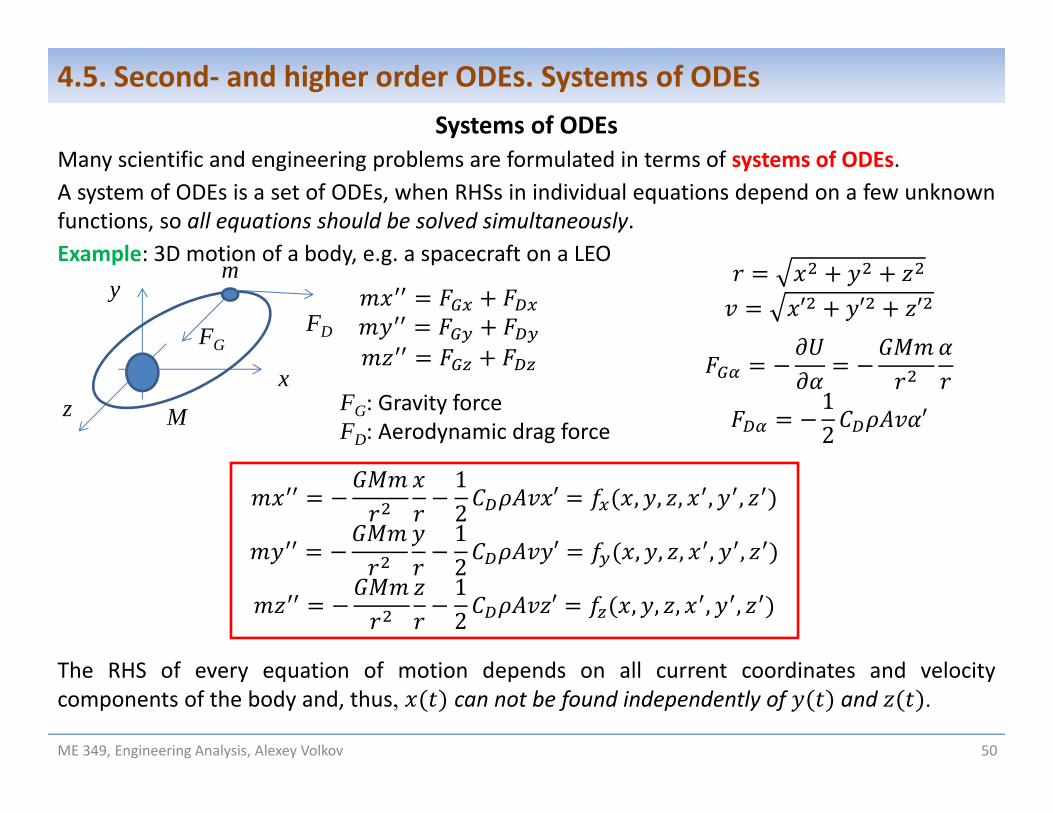
Systems of ODEsMany scientific and engineering problems are formulated in terms of systems of ODEs.A system of ODEs is a set of ODEs, when RHSs in individual equations depend on a few unknownfunctions, so all equations should be solved simultaneously.Example: 3D motion of a body, e.g. a spacecraft on a LEO
12 ′ , , , , ,12 ′ , , , , ,12 ′ , , , , ,
The RHS of every equation of motion depends on all current coordinates and velocitycomponents of the body and, thus, can not be found independently of and .
m
M
FDFG
x
y
z FG: Gravity forceFD: Aerodynamic drag force
′ ′ ′
12 ′
4.5. Second‐ and higher order ODEs. Systems of ODEs
ME 349, Engineering Analysis, Alexey Volkov 51
Fundamental systems of ODEsAmong all systems of ODEs, the systems of the first‐order equations in the explicit form play afundamental role.
This is the n‐dimensional fundamental system, i.e. a system of first‐order ODEs written in theexplicit form. The dimension of a fundamental system of ODEs is the number of unknownfunctions (equations).General solution of system (4.5.5) is the system of functions
, , … , , …, , , … ,
which turn every ODE in (4.5.5) into identity. Every function includes arbitrary constants , …,. These constants can be determined from the initial conditions of the initial value problem:
, , , , , .
Systems (4.5.6) are called fundamental, because any system (or individual equation) in theexplicit form reduces to a system of form (4.5.6) by a proper change of variables.
, , ,…, , , ,…,
…
, , ,…, , , ,…,
(4.5.5)
4.5. Second‐ and higher order ODEs. Systems of ODEs
(4.5.6)
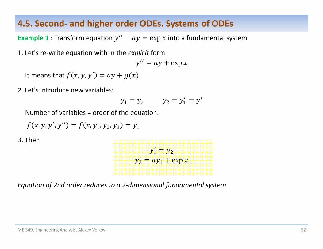
Example 1 : Transform equation exp into a fundamental system
1. Let's re‐write equation with in the explicit formexp
It means that , , .
2. Let's introduce new variables:,
Number of variables = order of the equation.
, , , , , ,
3. Then
exp
Equation of 2nd order reduces to a 2‐dimensional fundamental system
ME 349, Engineering Analysis, Alexey Volkov 52
4.5. Second‐ and higher order ODEs. Systems of ODEs
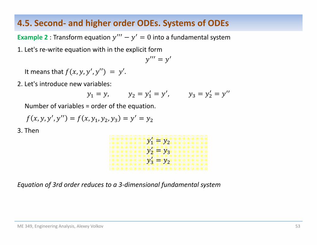
Example 2 : Transform equation 0 into a fundamental system
1. Let's re‐write equation with in the explicit form
It means that , , , ′′ ′.
2. Let's introduce new variables:, ,
Number of variables = order of the equation.
, , , , , ,
3. Then
Equation of 3rd order reduces to a 3‐dimensional fundamental system
ME 349, Engineering Analysis, Alexey Volkov 53
4.5. Second‐ and higher order ODEs. Systems of ODEs
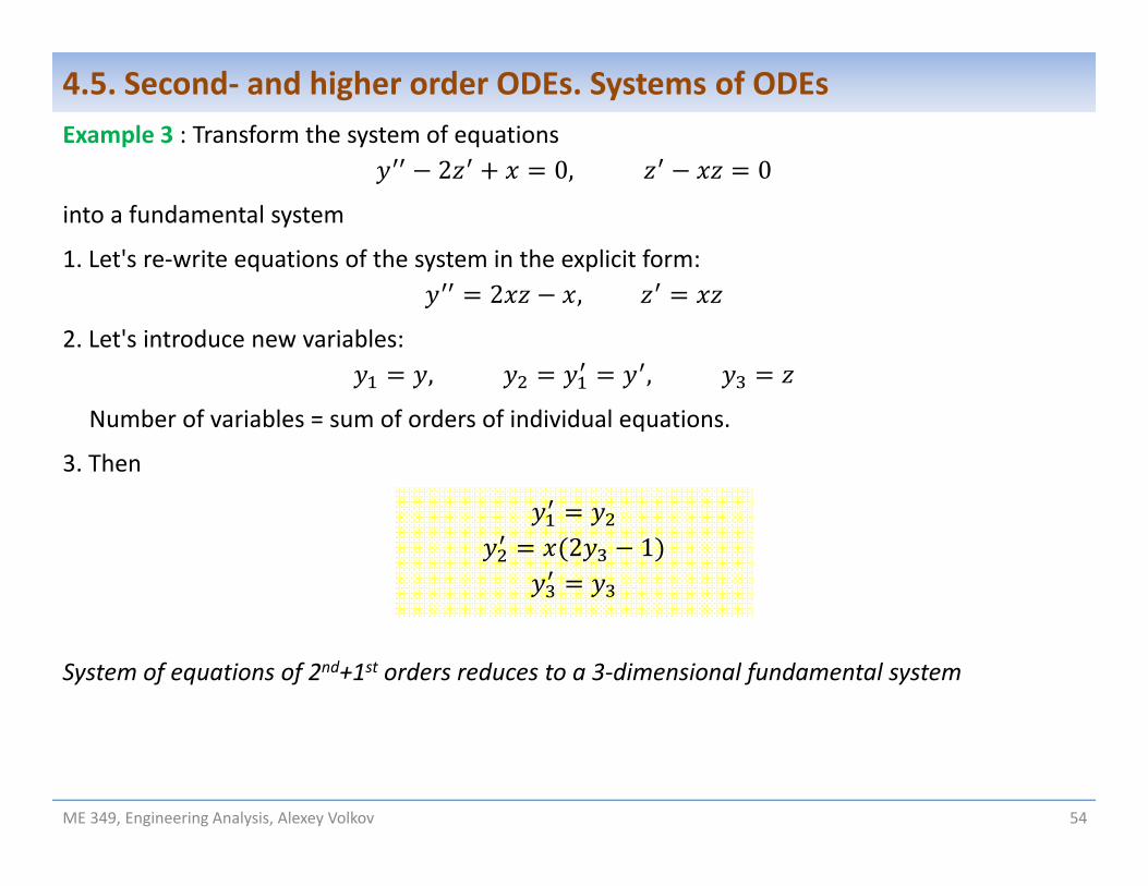
Example 3 : Transform the system of equations2 0, 0
into a fundamental system
1. Let's re‐write equations of the system in the explicit form:2 ,
2. Let's introduce new variables:, ,
Number of variables = sum of orders of individual equations.
3. Then
2 1
System of equations of 2nd+1st orders reduces to a 3‐dimensional fundamental system
ME 349, Engineering Analysis, Alexey Volkov 54
4.5. Second‐ and higher order ODEs. Systems of ODEs
ME 349, Engineering Analysis, Alexey Volkov 55
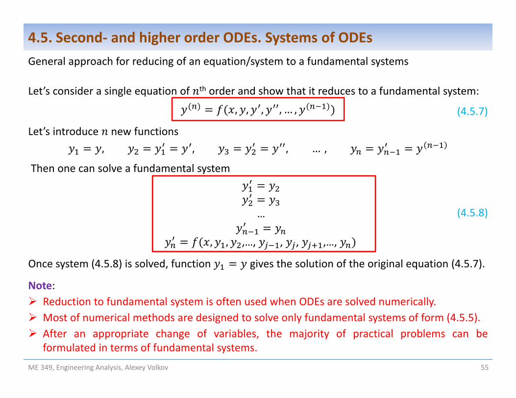
General approach for reducing of an equation/system to a fundamental systems
Let’s consider a single equation of th order and show that it reduces to a fundamental system:
, , , , … ,
Let’s introduce new functions, , , … ,
Then one can solve a fundamental system
Once system (4.5.8) is solved, function gives the solution of the original equation (4.5.7).
Note: Reduction to fundamental system is often used when ODEs are solved numerically. Most of numerical methods are designed to solve only fundamental systems of form (4.5.5). After an appropriate change of variables, the majority of practical problems can be
formulated in terms of fundamental systems.
…
, , ,…, , , ,…,
(4.5.7)
(4.5.8)
4.5. Second‐ and higher order ODEs. Systems of ODEs
ME 349, Engineering Analysis, Alexey Volkov 56
Matrix notation for fundamental systemsFundamental systems
are often formulated and solved using the matrix notation: Let’s introduce column vectors ofunknowns , their derivatives ′, and RHSs :
… , ′
…′, … ,
Then the fundamental system (4.5.6) can be written as
,
The vector notation, Eq. (4.5.9), allows us to write an arbitrary fundamental system in theform that is similar to the single first‐order ODE in the explicit form
′ , The vector notation is especially useful in two cases:
1. When we have many equations ( >>1) with unified RHSs.2. For numerical solution of fundamental systems, since it allows one to develop universal
computer codes, which can be applied to systems with arbitrary number of equations.
, , ,…, , , ,…,
…
, , ,…, , , ,…,
4.5. Second‐ and higher order ODEs. Systems of ODEs
(4.5.9)
ME 349, Engineering Analysis, Alexey Volkov 57
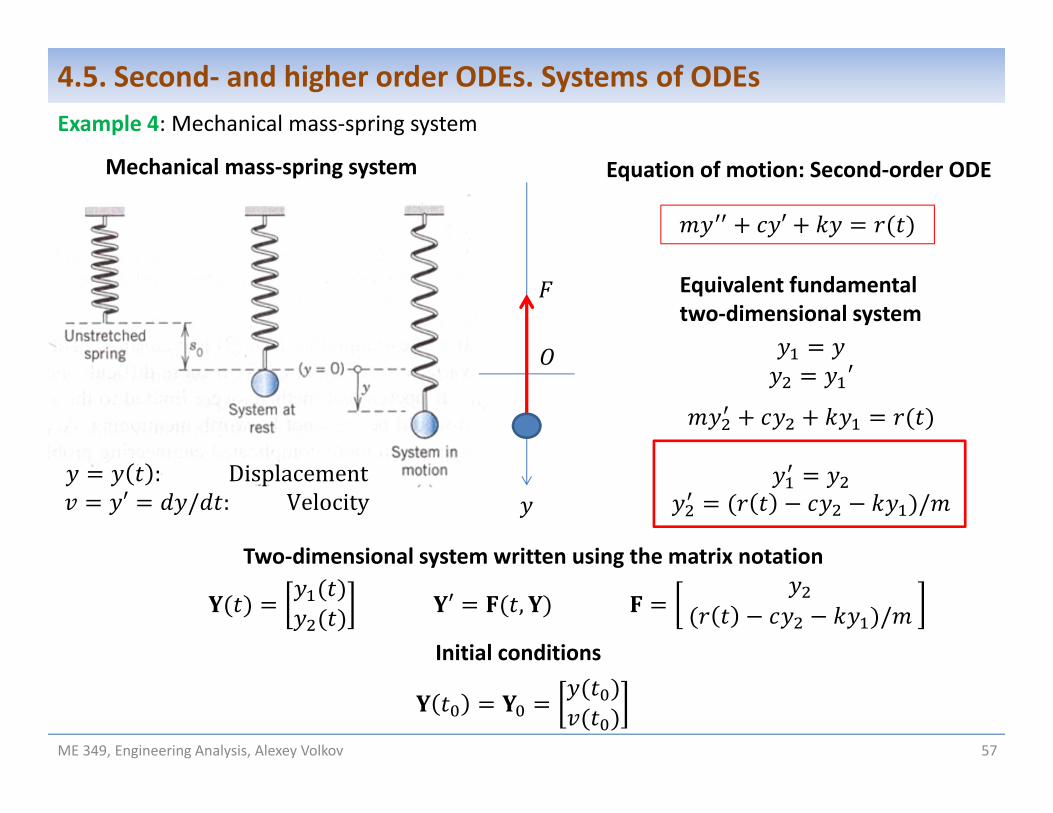
Mechanical mass‐spring system
: Displacement′ / : Velocity
′
Example 4: Mechanical mass‐spring system
4.5. Second‐ and higher order ODEs. Systems of ODEs
Equation of motion: Second‐order ODE
Equivalent fundamental two‐dimensional system
′
/
′ , /
Two‐dimensional system written using the matrix notation
Initial conditions
ME 349, Engineering Analysis, Alexey Volkov 58
4.6. Numerical methods for initial value problems (systems of ODEs) Numerical methods IVPs for fundamental systems of ODEs Runge‐Kutta methods of the second order for systems of ODEs Oscillations in the mass‐spring system. Resonance. Beats
Reading assignmentGilat 9.4
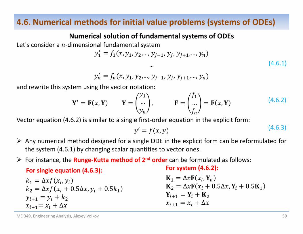
Numerical solution of fundamental systems of ODEsLet's consider a ‐dimensional fundamental system
, , ,…, , , ,…,
…
, , ,…, , , ,…,
and rewrite this system using the vector notation:
, … , … ,
Vector equation (4.6.2) is similar to a single first‐order equation in the explicit form:′ ,
Any numerical method designed for a single ODE in the explicit form can be reformulated forthe system (4.6.1) by changing scalar quantities to vector ones.
For instance, the Runge‐Kutta method of 2nd order can be formulated as follows:For single equation (4.6.3):
4.6. Numerical methods for initial value problems (systems of ODEs)
(4.6.1)
(4.6.3)
Four steps to solve numerically an IVP for a higher‐order ODE or a system of ODES
ME 349, Engineering Analysis, Alexey Volkov 60
4.6. Numerical methods for initial value problems (systems of ODEs)
, ,
/
, , /
∆ , ∆ 0.5∆ , 0.5 ∆
3. Re‐write fundamental system in the vector form
2. Introduce new functions and transform Equation/System to an equivalent fundamental system
1. Re‐write Equation/System in the explicit form
4. Apply integrators (Euler, RK2, etc.) developed for individual ODE in the
vector form
ME 349, Engineering Analysis, Alexey Volkov 61
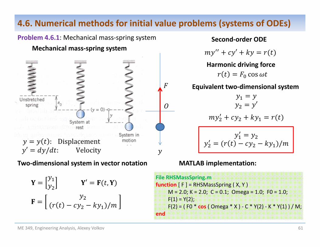
Mechanical mass‐spring system
: Displacement′ / : Velocity
′
Problem 4.6.1: Mechanical mass‐spring system
4.6. Numerical methods for initial value problems (systems of ODEs)
Second‐order ODE
Equivalent two‐dimensional system
′
/
′ ,
/
Two‐dimensional system in vector notation MATLAB implementation:
File RHSMassSpring.mfunction [ F ] = RHSMassSpring ( X, Y )
M = 2.0; K = 2.0; C = 0.1; Omega = 1.0; F0 = 1.0; F(1) = Y(2);F(2) = ( F0 * cos ( Omega * X ) ‐ C * Y(2) ‐ K * Y(1) ) / M;
end
cosHarmonic driving force
62
4.6. Numerical methods for initial value problems (systems of ODEs)
ME 349, Engineering Analysis, Alexey Volkov
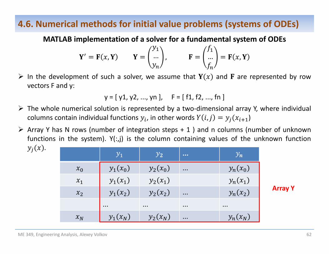
MATLAB implementation of a solver for a fundamental system of ODEs
, … , … ,
In the development of such a solver, we assume that and are represented by rowvectors F and y:
y = [ y1, y2, ..., yn ], F = [ f1, f2, ..., fn ] The whole numerical solution is represented by a two‐dimensional array Y, where individual
columns contain individual functions , in other words , )
Array Y has N rows (number of integration steps + 1 ) and n columns (number of unknownfunctions in the system). Y(:,j) is the column containing values of the unknown function
....
...
...
... ... ... ...
...
Array Y
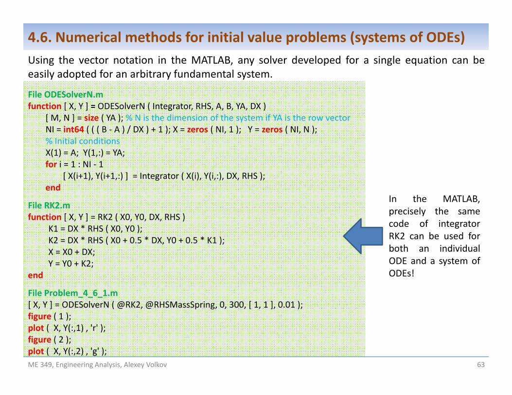
Using the vector notation in the MATLAB, any solver developed for a single equation can beeasily adopted for an arbitrary fundamental system.
File ODESolverN.mfunction [ X, Y ] = ODESolverN ( Integrator, RHS, A, B, YA, DX )
[ M, N ] = size ( YA ); % N is the dimension of the system if YA is the row vectorNI = int64 ( ( ( B ‐ A ) / DX ) + 1 ); X = zeros ( NI, 1 ); Y = zeros ( NI, N ); % Initial conditionsX(1) = A; Y(1,:) = YA;for i = 1 : NI ‐ 1
4.6. Numerical methods for initial value problems (systems of ODEs)
ME 349, Engineering Analysis, Alexey Volkov
In the MATLAB,precisely the samecode of integratorRK2 can be used forboth an individualODE and a system ofODEs!
ME 349, Engineering Analysis, Alexey Volkov 64
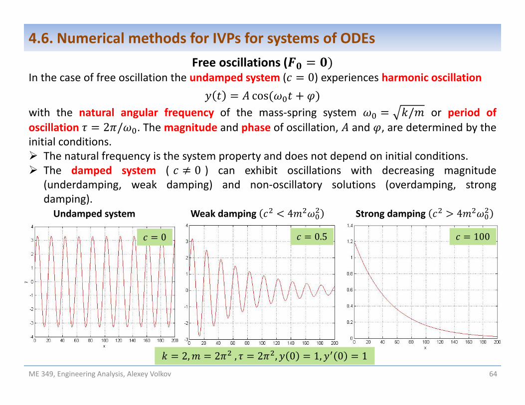
Free oscillations (In the case of free oscillation the undamped system ( 0) experiences harmonic oscillation
coswith the natural angular frequency of the mass‐spring system / or period ofoscillation 2 / . Themagnitude and phase of oscillation, and , are determined by theinitial conditions. The natural frequency is the system property and does not depend on initial conditions. The damped system ( 0 ) can exhibit oscillations with decreasing magnitude
(underdamping, weak damping) and non‐oscillatory solutions (overdamping, strongdamping).Undamped system Weak damping 4 Strong damping 4
4.6. Numerical methods for IVPs for systems of ODEs
0 0.5 100
2, 2 , 2 , 0 1, 0 1
ME 349, Engineering Analysis, Alexey Volkov 65
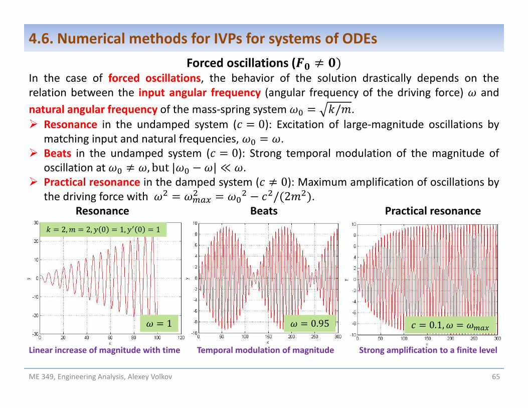
Forced oscillations (In the case of forced oscillations, the behavior of the solution drastically depends on therelation between the input angular frequency (angular frequency of the driving force) andnatural angular frequency of the mass‐spring system / . Resonance in the undamped system ( 0): Excitation of large‐magnitude oscillations by
matching input and natural frequencies, . Beats in the undamped system ( 0): Strong temporal modulation of the magnitude of
oscillation at , but| | ≪ . Practical resonance in the damped system ( 0): Maximum amplification of oscillations by
the driving force with / 2 .Resonance Beats Practical resonance
Linear increase of magnitude with time Temporal modulation of magnitude Strong amplification to a finite level
4.6. Numerical methods for IVPs for systems of ODEs
0.951 0.1,
2, 2, 0 1, 0 1
ME 349, Engineering Analysis, Alexey Volkov 66
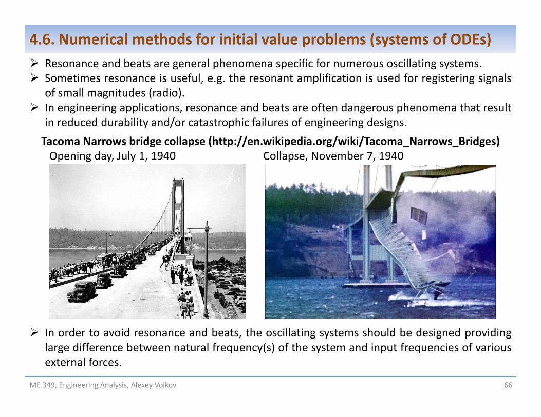
Resonance and beats are general phenomena specific for numerous oscillating systems. Sometimes resonance is useful, e.g. the resonant amplification is used for registering signals
of small magnitudes (radio). In engineering applications, resonance and beats are often dangerous phenomena that result
in reduced durability and/or catastrophic failures of engineering designs.Tacoma Narrows bridge collapse (http://en.wikipedia.org/wiki/Tacoma_Narrows_Bridges)Opening day, July 1, 1940 Collapse, November 7, 1940
In order to avoid resonance and beats, the oscillating systems should be designed providinglarge difference between natural frequency(s) of the system and input frequencies of variousexternal forces.
4.6. Numerical methods for initial value problems (systems of ODEs)
ME 349, Engineering Analysis, Alexey Volkov 67
4.7. Numerical solution of IVPs with build‐in MATLAB solvers MATLAB build‐in solvers for systems of ODEs Example: Simple pendulum Example: Double pendulum
Reading assignmentGilat 9.4
ME 349, Engineering Analysis, Alexey Volkov 68
4.7. Numerical solution of IVPs with build‐in MATLAB solversMATLAB build‐in solvers for systems of ODEs
Any build‐in MATLAB solver for IVPs can be used to solve fundamental systems of ODEs. [ x, y ] = Solver ( @RHS, xspan, ya )
RHS in the function that implements calculation of the RHS , , where y is a vector. xspan is 1D array that should contain at least two real values. The first and last elements
of xspan are used as limits of the integration interval , . ya is the initial condition (vector) at x = a. x is the column vector with nodal values of x obtained as a result of integration. y is a 2D vector. Individual columns y(:,1), y(:,2),…, correspond to numerical solutions
for , , ... The RHS function should be programmed assuming that the F is the column vector!
Problem 4.7.1: Solution of ODEs for the mass‐spring system with ode45 solver:
Transpose changes the shape of vector F from
row to column
File RHSMassSpring.mfunction [ F ] = MassSpringEq2 ( X, Y )
M = 2.0; K = 2.0; C = 0.1; Omega = 1.0; F0 = 1.0; F(1) = Y(2);F(2) = ( F0 * cos ( Omega * X ) ‐ C * Y(2) ‐ K * Y(1) ) / M;F = F';
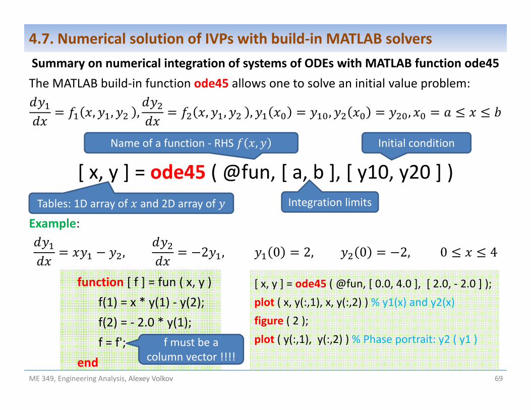
Summary on numerical integration of systems of ODEs with MATLAB function ode45The MATLAB build‐in function ode45 allows one to solve an initial value problem:
, , , , , , , ,
[ x, y ] = ode45 ( @fun, [ a, b ], [ y10, y20 ] )
Example:
, 2 , 0 2, 0 2, 0 4
function [ f ] = fun ( x, y )f(1) = x * y(1) ‐ y(2);f(2) = ‐ 2.0 * y(1);f = f';
endME 349, Engineering Analysis, Alexey Volkov 69
4.7. Numerical solution of IVPs with build‐in MATLAB solvers
Name of a function ‐ RHS ,
Integration limits
Initial condition
Tables: 1D array of and 2D array of
[ x, y ] = ode45 ( @fun, [ 0.0, 4.0 ], [ 2.0, ‐ 2.0 ] );plot ( x, y(:,1), x, y(:,2) ) % y1(x) and y2(x)figure ( 2 );plot ( y(:,1), y(:,2) ) % Phase portrait: y2 ( y1 )f must be a
column vector !!!!
ME 349, Engineering Analysis, Alexey Volkov 70
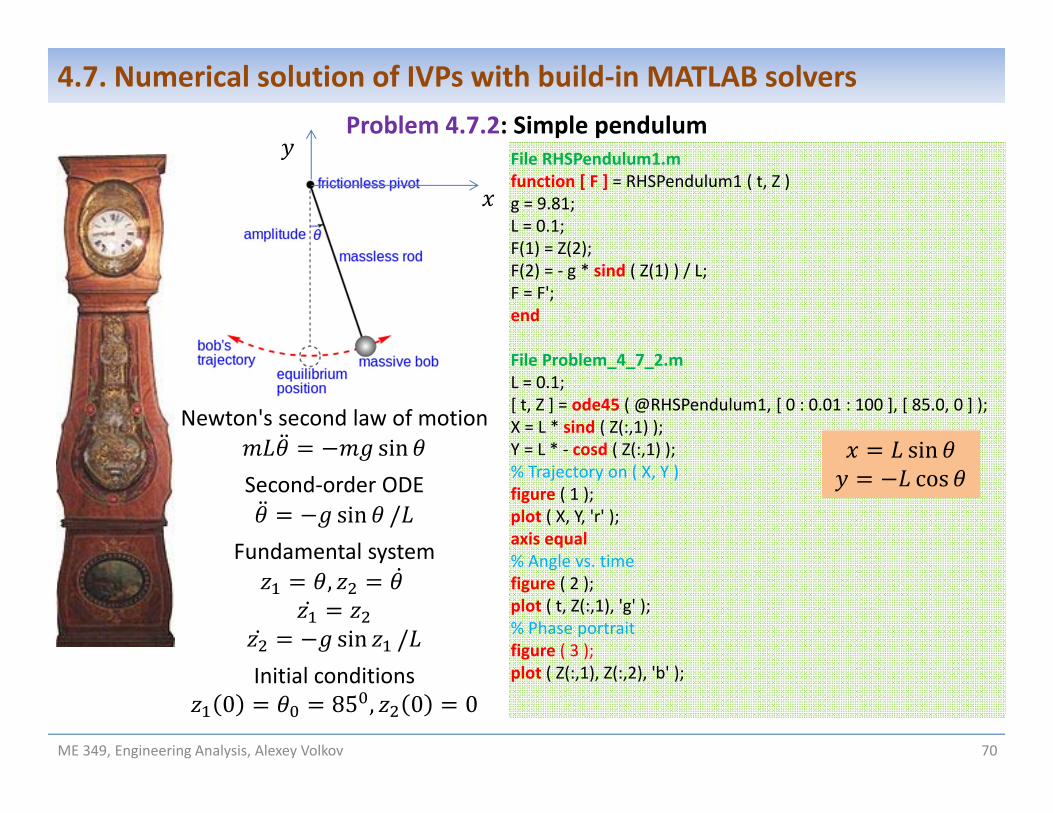
4.7. Numerical solution of IVPs with build‐in MATLAB solversProblem 4.7.2: Simple pendulum
File RHSPendulum1.mfunction [ F ] = RHSPendulum1 ( t, Z )g = 9.81;L = 0.1;F(1) = Z(2);F(2) = ‐ g * sind ( Z(1) ) / L;F = F';end
File Problem_4_7_2.mL = 0.1;[ t, Z ] = ode45 ( @RHSPendulum1, [ 0 : 0.01 : 100 ], [ 85.0, 0 ] );X = L * sind ( Z(:,1) );Y = L * ‐ cosd ( Z(:,1) );% Trajectory on ( X, Y )figure ( 1 );plot ( X, Y, 'r' );axis equal% Angle vs. timefigure ( 2 );plot ( t, Z(:,1), 'g' );% Phase portrait figure ( 3 );plot ( Z(:,1), Z(:,2), 'b' );
Newton's second law of motionsin
Second‐order ODEsin /
Fundamental system,
sin /Initial conditions
0 85 , 0 0
sincos
ME 349, Engineering Analysis, Alexey Volkov 71
4.7. Numerical solution of IVPs with build‐in MATLAB solversSingle pendulum: Numerical solution
0.1
sin /Initial conditions
0 85 , 0 0
ME 349, Engineering Analysis, Alexey Volkov 72
4.7. Numerical solution of IVPs with build‐in MATLAB solversProblem 4.7.3: Double pendulum
Double pendulum demonstrates unpredictable behavior This is the simple example of mechanical chaotic system
Bobs
Rigid massless strings
ME 349, Engineering Analysis, Alexey Volkov 73
4.7. Numerical solution of IVPs with build‐in MATLAB solversDouble pendulum: Equations of motion
Newton's second law of motion
sin sin
cos cos
Newton's second law of motion
sin
cos
Forces applied to bob 1 Forces applied to bob 2
ME 349, Engineering Analysis, Alexey Volkov 74
4.7. Numerical solution of IVPs with build‐in MATLAB solversDouble pendulum: Reduction to a fundamental system (optional slide 1)
sin sin
cos cos
sin
cos
We obtained 4 equations of motion, Eqs. (1)‐(4). However, we can reduce these equations to 2 equations,
because lengths of strings are constant. For this purpose we need to do 2 steps
1. Exclude from equations of motion string tensions and .
2. Derive , , , in terms of and . Then we will get 2 equations with respect to and .
Step 1(1)
(2)
(3)
(4)
Add Eq. (1) to Eq. (3) and Eq. (2) to Eq. (4)
sin
cos
cos+
sin
cos+
sincos sin sin
cos sin
sin
ME 349, Engineering Analysis, Alexey Volkov 75
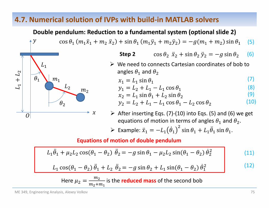
4.7. Numerical solution of IVPs with build‐in MATLAB solversDouble pendulum: Reduction to a fundamental system (optional slide 2)
Step 2 cos sin sin
cos sin sin
sincos
sin sincos cos
After inserting Eqs. (7)‐(10) into Eqs. (5) and (6) we get equations of motion in terms of angles and .
Example: sin sin .
(7)(8)(9)(10)
(5)
(6)
(11)
(12)
cos sin sin
cos sin sin
Equations of motion of double pendulum
Here is the reduced mass of the second bob
We need to connects Cartesian coordinates of bob to angles and
ME 349, Engineering Analysis, Alexey Volkov 76
4.7. Numerical solution of IVPs with build‐in MATLAB solversDouble pendulum: Reduction to a fundamental system (optional slide 3)
Reduction of equations of motion to explicit form
cos sin sin
cos sin sin
These equations can be re‐written in the matrix form as follows:
coscos
sin sinsin sin
(13)
SLE given by Eq. (13) can be solved as , where A is calculated with Kramer’s rule:
, (14)
ME 349, Engineering Analysis, Alexey Volkov 77
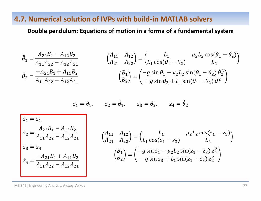
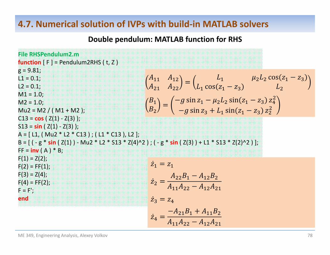
4.7. Numerical solution of IVPs with build‐in MATLAB solversDouble pendulum: Equations of motion in a forma of a fundamental system
4.7. Numerical solution of IVPs with build‐in MATLAB solversDouble pendulum: MATLAB function for RHS
coscos
sin sinsin sin
ME 349, Engineering Analysis, Alexey Volkov 79
4.7. Numerical solution of IVPs with build‐in MATLAB solversDouble pendulum: MATLAB script
File Problem_4_7_3.m% Here we set lengths of stringsL1 = 0.1;L2 = 0.1;
% Here we use ode45 solver to obtain angles[ t, Z ] = ode45 ( @RHSPendulum2, [ 0 : 0.01 : 20 ], [ ( degtorad ( 90.0 ) ), 0, ( degtorad ( 90.0 ) ), 0 ] );
% Now we have Z solution of equations of motions:% Z(1) = Theta_1% Z(2) = d Theta_1 / d t% Z(3) = Theta_2% Z(4) = d Theta_3 / d t
% Here we convert angles into Cartesian coordinates of bob 1X1 = L1 * sin ( Z(:,1) );Y1 = L1 + L2 ‐ L1 * cos ( Z(:,1) );
% Here we convert angles into Cartesian coordinates of bob 2X2 = L1 * sin ( Z(:,1) ) + L2 * sin ( Z(:,3) );Y2 = L1 + L2 ‐ L1 * cos ( Z(:,1) ) ‐ L2 * cos ( Z(:,3) );
% Now we can choose one of two ways to visualize solutions
% Script Pendulum2Animation animates the motion of pendulum on the plane (X,Y)Pendulum2Animation
Eq. (7)‐1(10):sin
cossin sin
cos cos
Initial conditions:0 0 90 , 0 0 0
ME 349, Engineering Analysis, Alexey Volkov 80
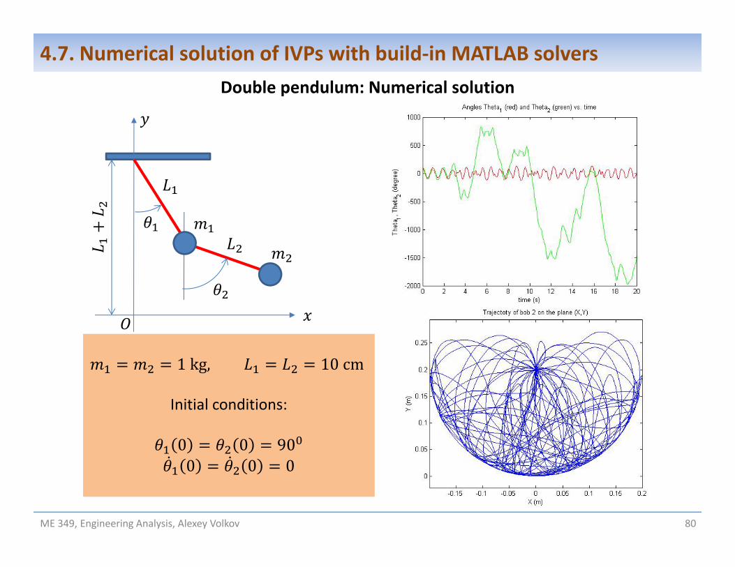
4.7. Numerical solution of IVPs with build‐in MATLAB solversDouble pendulum: Numerical solution
1kg, 10cm
Initial conditions:
0 0 900 0 0
ME 349, Engineering Analysis, Alexey Volkov 81
4.8. SummaryFor the exam we must know how To calculate numerically the first derivatives with forward, backward, and central differences
of the first and second order. To calculate numerically the second derivatives with central‐difference equation. To implement calculations of the above derivatives in the MATLAB code. To numerically integrate a function with the rectangle and trapezoidal rules. To implement the rectangle and trapezoidal rules in the MATLAB code. To numerically integrate a function with the MATLAB quad functions. To use Euler, RK2, and RK4 methods for numerical solution of individual first‐order ODEs. To use ode45 solver for numerical solution of individual first‐order ODEs. To use the Euler, RK2, and RK4 methods for numerical solution of fundamental systems of
ODEs. To use ode45 solver for numerical solution of fundamental systems of ODEs. To re‐write a higher‐order ODE or a system in the form of a fundamental system of ODEs
using the matrix notation, To formulate and solve numerically the equations of the mechanical mass‐spring system. To know conditions, when resonance, beats, and practical resonance occur in the mass‐
spring system. To formulate and solve numerically the equations of the single pendulum.


![Arduino Programming Part 1 - start [ME 120]me120.mme.pdx.edu/lib/exe/...media=lecture:arduino_programming_1.pdfME 120: Arduino Programming Overview Arduino Environment Basic code components](https://static.documents.pub/doc/80x56/5ab835057f8b9ad3038c8a6d/arduino-programming-part-1-start-me-120me120mmepdxedulibexemedialecturearduinoprogramming1pdfme.jpg)


