1
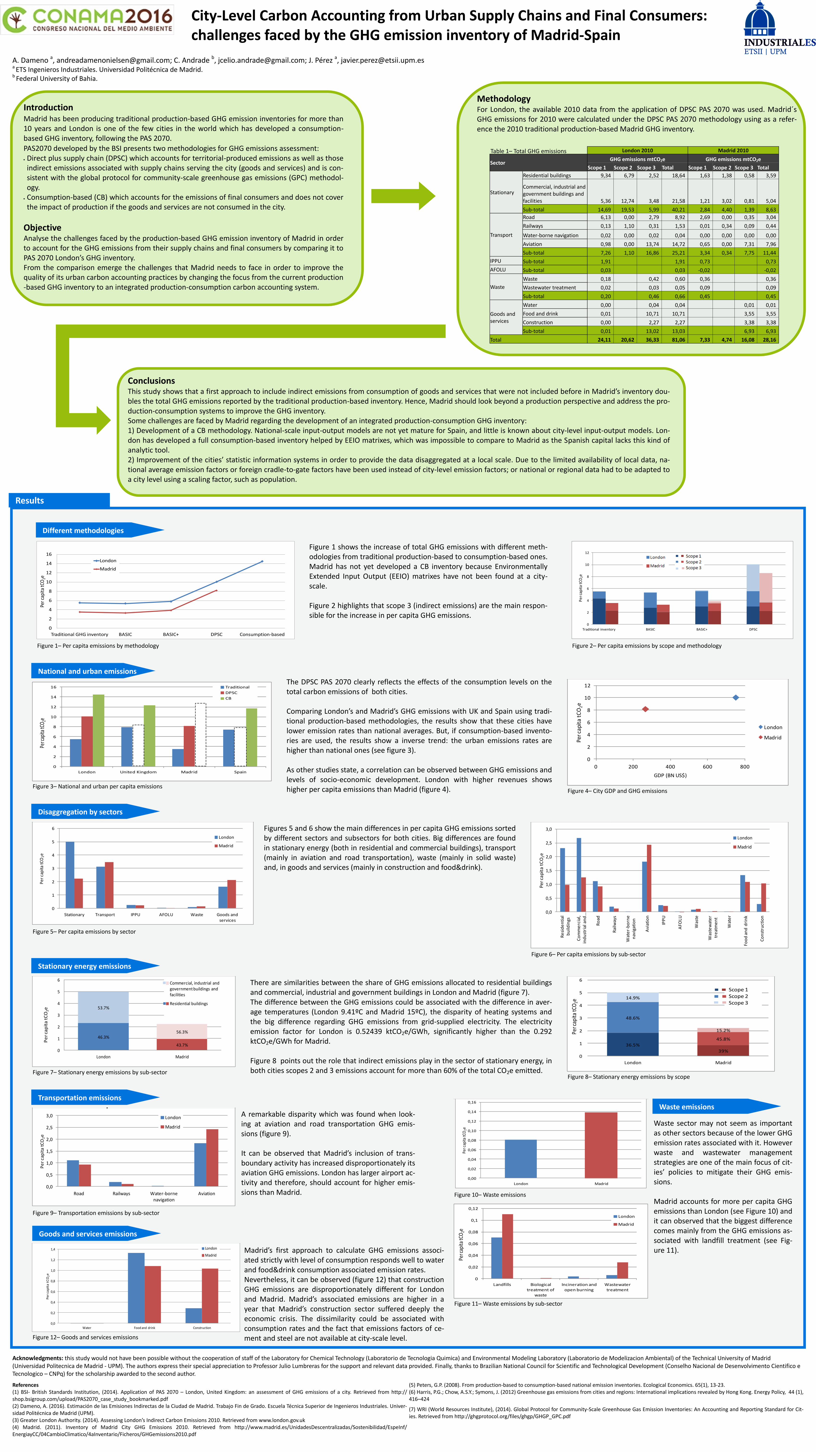
City-Level Carbon Accounting from Urban Supply Chains and Final Consumers: challenges faced by the GHG emission inventory of Madrid-Spain A. Dameno a , [email protected]; C. Andrade b , [email protected]; J. Pérez a , [email protected] a ETS Ingenieros Industriales. Universidad Politécnica de Madrid. b Federal University of Bahia. Acknowledgments: this study would not have been possible without the cooperation of staff of the Laboratory for Chemical Technology (Laboratorio de Tecnologia Quimica) and Environmental Modeling Laboratory (Laboratorio de Modelizacion Ambiental) of the Technical University of Madrid (Universidad Politecnica de Madrid - UPM). The authors express their special appreciation to Professor Julio Lumbreras for the support and relevant data provided. Finally, thanks to Brazilian National Council for Scientific and Technological Development (Conselho Nacional de Desenvolvimento Cientifico e Tecnologico – CNPq) for the scholarship awarded to the second author. References (1) BSI- British Standards Institution, (2014). Application of PAS 2070 – London, United Kingdom: an assessment of GHG emissions of a city. Retrieved from http:// shop.bsigroup.com/upload/PAS2070_case_study_bookmarked.pdf (2) Dameno, A. (2016). Estimación de las Emisiones Indirectas de la Ciudad de Madrid. Trabajo Fin de Grado. Escuela Técnica S uperior de Ingenieros Industriales. Univer- sidad Politécnica de Madrid (UPM). (3) Greater London Authority. (2014). Assessing London’s Indirect Carbon Emissions 2010. Retrieved from www.london.gov.uk (4) Madrid. (2011). Inventory of Madrid City GHG Emissions 2010. Retrieved from http://www.madrid.es/UnidadesDescentralizadas/Sostenibilidad/EspeInf/ EnergiayCC/04CambioClimatico/4aInventario/Ficheros/GHGemissions2010.pdf (5) Peters, G.P. (2008). From production-based to consumption-based national emission inventories. Ecological Economics. 65(1), 13-23. (6) Harris, P.G.; Chow, A.S.Y.; Symons, J. (2012) Greenhouse gas emissions from cities and regions: International implications revealed by Hong Kong. Energy Policy, 44 (1), 416–424 (7) WRI (World Resources Institute), (2014). Global Protocol for Community-Scale Greenhouse Gas Emission Inventories: An Accounting and Reporting Standard for Cit- ies. Retrieved from http://ghgprotocol.org/files/ghgp/GHGP_GPC.pdf Introduction Madrid has been producing traditional production-based GHG emission inventories for more than 10 years and London is one of the few cities in the world which has developed a consumption- based GHG inventory, following the PAS 2070. PAS2070 developed by the BSI presents two methodologies for GHG emissions assessment: Direct plus supply chain (DPSC) which accounts for territorial-produced emissions as well as those indirect emissions associated with supply chains serving the city (goods and services) and is con- sistent with the global protocol for community-scale greenhouse gas emissions (GPC) methodol- ogy. Consumption-based (CB) which accounts for the emissions of final consumers and does not cover the impact of production if the goods and services are not consumed in the city. Objective Analyse the challenges faced by the production-based GHG emission inventory of Madrid in order to account for the GHG emissions from their supply chains and final consumers by comparing it to PAS 2070 London’s GHG inventory. From the comparison emerge the challenges that Madrid needs to face in order to improve the quality of its urban carbon accounting practices by changing the focus from the current production -based GHG inventory to an integrated production-consumption carbon accounting system. Conclusions This study shows that a first approach to include indirect emissions from consumption of goods and services that were not included before in Madrid’s inventory dou- bles the total GHG emissions reported by the traditional production-based inventory. Hence, Madrid should look beyond a production perspective and address the pro- duction-consumption systems to improve the GHG inventory. Some challenges are faced by Madrid regarding the development of an integrated production-consumption GHG inventory: 1) Development of a CB methodology. National-scale input-output models are not yet mature for Spain, and little is known about city-level input-output models. Lon- don has developed a full consumption-based inventory helped by EEIO matrixes, which was impossible to compare to Madrid as the Spanish capital lacks this kind of analytic tool. 2) Improvement of the cities’ statistic information systems in order to provide the data disaggregated at a local scale. Due to the limited availability of local data, na- tional average emission factors or foreign cradle-to-gate factors have been used instead of city-level emission factors; or national or regional data had to be adapted to a city level using a scaling factor, such as population. Methodology For London, the available 2010 data from the application of DPSC PAS 2070 was used. Madrid´s GHG emissions for 2010 were calculated under the DPSC PAS 2070 methodology using as a refer- ence the 2010 traditional production-based Madrid GHG inventory. London 2010 Madrid 2010 Sector GHG emissions mtCO 2 e GHG emissions mtCO 2 e Scope 1 Scope 2 Scope 3 Total Scope 1 Scope 2 Scope 3 Total Stationary Residential buildings 9,34 6,79 2,52 18,64 1,63 1,38 0,58 3,59 Commercial, industrial and government buildings and facilities 5,36 12,74 3,48 21,58 1,21 3,02 0,81 5,04 Sub-total 14,69 19,53 5,99 40,21 2,84 4,40 1,39 8,63 Transport Road 6,13 0,00 2,79 8,92 2,69 0,00 0,35 3,04 Railways 0,13 1,10 0,31 1,53 0,01 0,34 0,09 0,44 Water-borne navigation 0,02 0,00 0,02 0,04 0,00 0,00 0,00 0,00 Aviation 0,98 0,00 13,74 14,72 0,65 0,00 7,31 7,96 Sub-total 7,26 1,10 16,86 25,21 3,34 0,34 7,75 11,44 IPPU Sub-total 1,91 1,91 0,73 0,73 AFOLU Sub-total 0,03 0,03 -0,02 -0,02 Waste Waste 0,18 0,42 0,60 0,36 0,36 Wastewater treatment 0,02 0,03 0,05 0,09 0,09 Sub-total 0,20 0,46 0,66 0,45 0,45 Goods and services Water 0,00 0,04 0,04 0,01 0,01 Food and drink 0,01 10,71 10,71 3,55 3,55 Construction 0,00 2,27 2,27 3,38 3,38 Sub-total 0,01 13,02 13,03 6,93 6,93 Total 24,11 20,62 36,33 81,06 7,33 4,74 16,08 28,16 Table 1– Total GHG emissions 0 2 4 6 8 10 12 14 16 Traditional GHG inventory BASIC BASIC+ DPSC Consumption-based Per capita tCO 2 e London Madrid Figure 1 shows the increase of total GHG emissions with different meth- odologies from traditional production-based to consumption-based ones. Madrid has not yet developed a CB inventory because Environmentally Extended Input Output (EEIO) matrixes have not been found at a city- scale. Figure 2 highlights that scope 3 (indirect emissions) are the main respon- sible for the increase in per capita GHG emissions. Figure 1– Per capita emissions by methodology Figure 2– Per capita emissions by scope and methodology 0 2 4 6 8 10 12 Traditional inventory BASIC BASIC+ DPSC Per capita tCO 2 e Different methodologies The DPSC PAS 2070 clearly reflects the effects of the consumption levels on the total carbon emissions of both cities. Comparing London’s and Madrid’s GHG emissions with UK and Spain using tradi- tional production-based methodologies, the results show that these cities have lower emission rates than national averages. But, if consumption-based invento- ries are used, the results show a inverse trend: the urban emissions rates are higher than national ones (see figure 3). As other studies state, a correlation can be observed between GHG emissions and levels of socio-economic development. London with higher revenues shows higher per capita emissions than Madrid (figure 4). Figure 3– National and urban per capita emissions Figure 4– City GDP and GHG emissions 0 2 4 6 8 10 12 0 200 400 600 800 Per capita tCO 2 e GDP (BN US$) London Madrid 0 2 4 6 8 10 12 14 16 London United Kingdom Madrid Spain Traditional DPSC CB Per capita tCO 2 e National and urban emissions Figures 5 and 6 show the main differences in per capita GHG emissions sorted by different sectors and subsectors for both cities. Big differences are found in stationary energy (both in residential and commercial buildings), transport (mainly in aviation and road transportation), waste (mainly in solid waste) and, in goods and services (mainly in construction and food&drink). 0,0 0,5 1,0 1,5 2,0 2,5 3,0 Residential buildings Commercial, industrial and … Road Railways Water-borne navigation Aviation IPPU AFOLU Waste Wastewater treatment Water Food and drink Construction Per capita tCO 2 e London Madrid Figure 5– Per capita emissions by sector Figure 6– Per capita emissions by sub-sector 0 1 2 3 4 5 6 Stationary Transport IPPU AFOLU Waste Goods and services Per capita tCO 2 e London Madrid Disaggregation by sectors There are similarities between the share of GHG emissions allocated to residential buildings and commercial, industrial and government buildings in London and Madrid (figure 7). The difference between the GHG emissions could be associated with the difference in aver- age temperatures (London 9.41ºC and Madrid 15ºC), the disparity of heating systems and the big difference regarding GHG emissions from grid-supplied electricity. The electricity emission factor for London is 0.52439 ktCO 2 e/GWh, significantly higher than the 0.292 ktCO 2 e/GWh for Madrid. Figure 8 points out the role that indirect emissions play in the sector of stationary energy, in both cities scopes 2 and 3 emissions account for more than 60% of the total CO 2 e emitted. Figure 7– Stationary energy emissions by sub-sector Figure 8– Stationary energy emissions by scope 46.3% 43.7% 53.7% 56.3% 0 1 2 3 4 5 6 London Madrid Commercial, industrial and government buildings and facilities Residential buildings Per capita tCO 2 e 36.5% 39% 48.6% 45.8% 14.9% 15.2% 0 1 2 3 4 5 6 London Madrid Per capita tCO 2 e Scope 1 Scope 2 Scope 3 Stationary energy emissions A remarkable disparity which was found when look- ing at aviation and road transportation GHG emis- sions (figure 9). It can be observed that Madrid’s inclusion of trans- boundary activity has increased disproportionately its aviation GHG emissions. London has larger airport ac- tivity and therefore, should account for higher emis- sions than Madrid. Figure 9– Transportation emissions by sub-sector 0,0 0,5 1,0 1,5 2,0 2,5 3,0 Road Railways Water-borne navigation Aviation Per capita tCO 2 e London Madrid Transportation emissions 0,00 0,02 0,04 0,06 0,08 0,10 0,12 0,14 0,16 London Madrid Per capita tCO 2 e Waste sector may not seem as important as other sectors because of the lower GHG emission rates associated with it. However waste and wastewater management strategies are one of the main focus of cit- ies’ policies to mitigate their GHG emis- sions. Madrid accounts for more per capita GHG emissions than London (see Figure 10) and it can observed that the biggest difference comes mainly from the GHG emissions as- sociated with landfill treatment (see Fig- ure 11). Figure 10– Waste emissions Figure 11– Waste emissions by sub-sector 0 0,02 0,04 0,06 0,08 0,1 0,12 Landfills Biological treatment of waste Incineration and open burning Wastewater treatment London Madrid Per capita tCO 2 e Waste emissions Madrid’s first approach to calculate GHG emissions associ- ated strictly with level of consumption responds well to water and food&drink consumption associated emission rates. Nevertheless, it can be observed (figure 12) that construction GHG emissions are disproportionately different for London and Madrid. Madrid’s associated emissions are higher in a year that Madrid’s construction sector suffered deeply the economic crisis. The dissimilarity could be associated with consumption rates and the fact that emissions factors of ce- ment and steel are not available at city-scale level. Figure 12– Goods and services emissions 0,0 0,2 0,4 0,6 0,8 1,0 1,2 1,4 Water Food and drink Construction Per capita tCO 2 e London Madrid Goods and services emissions Results