4 The gravity model in international trade Luca De Benedictis and Daria Taglioni Luca De Benedictis: DIEF, University of Macerata, Via Crescimbeni 20, 62100 Macerata, Italy. E-mail: [email protected]. Daria Taglioni: ECB, Frankfurt am Main, Germany and Centre for Economic and Trade Integration at The Graduate Institute of International and Development Studies, Rue de Lausanne 132, 1211 Geneva, Switzerland. E-mail: [email protected]Abstract Since Jan Tinberben’s original formulation (Tinbergen 1962), the empir- ical analysis of bilateral trade flows through the estimation of a gravity equation has gone a long way. It has acquired a solid reputation of good fitting; it gained respected micro foundations that allowed it to move to a mature stage in which the “turn-over” gravity equation has been replaced by a gravity model; and it has dominated the literature on trade policy evaluation. In this chapter we show how some of the issues raised by Tinbergen have been the step stones of a 50-year long research agenda, and how the numerous empirical and theoretical contributions that followed dealt with old problems and highlighted new ones. Some future promising research issues are finally indicated.
Transcript
4 The gravity model in international trade
Luca De Benedictis and Daria Taglioni
Luca De Benedictis: DIEF, University of Macerata, Via Crescimbeni 20, 62100 Macerata, Italy. E-mail: [email protected].
Daria Taglioni: ECB, Frankfurt am Main, Germany and Centre for Economic and Trade Integration at The Graduate Institute of International and Development Studies, Rue de Lausanne 132, 1211 Geneva, Switzerland. E-mail: [email protected]
Abstract Since Jan Tinberben’s original formulation (Tinbergen 1962), the empir-ical analysis of bilateral trade flows through the estimation of a gravity equation has gone a long way. It has acquired a solid reputation of good fitting; it gained respected micro foundations that allowed it to move to a mature stage in which the “turn-over” gravity equation has been replaced by a gravity model; and it has dominated the literature on trade policy evaluation. In this chapter we show how some of the issues raised by Tinbergen have been the step stones of a 50-year long research agenda, and how the numerous empirical and theoretical contributions that followed dealt with old problems and highlighted new ones. Some future promising research issues are finally indicated.
2
4.1 Introduction
When in 1962 Jan Tinbergen, the future winner of the first 1969 Alfred Nobel Me-morial Prize for economics, was sketching the empirical analysis for a report fi-nanced by a New York-based philanthropic foundation, his mind was back at his college years. In 1929 he had received his PhD in physics from Leiden University, the Netherlands, with a thesis entitled Minimum Problems in Physics and Economics under the supervision of Paul Ehrenfest, a close friend of Albert Einstein’s (Szen-berg 1992, p. 276; Leen 2004). Theoretical physics was his bread and butter, before the concern for the causes of poverty of the local working class pressed him to switch to economics. Therefore, it must not come as a surprise that, when he had to propose to the team of fellow colleagues of the Netherlands Economic Institute an econometric exercise “to determine the normal or standard pattern of international trade that would prevail in the absence of trade impediments”, he came out with the idea of an econometric model formulated along the lines of Newton’s law of gravi-ty.1
All simple and successful ideas have a life of their own, and their paternity can be attributed to multiple individuals. Before Tinbergen, Ravenstein (1885) and Zipf (1946) used gravity concepts to model migration flows. Independently from Tinber-gen, Pöyhönen (1963), inspired by Leo Tornqvist,2 published a paper using a similar approach.3 Tinbergen’s student and team-member of the Netherlands Economic In-stitute, Hans Linnemann, published a follow-up study (Linnemann 1966) which ex-tended the analysis and discussed the theoretical basis of the gravity equation using the Walrasian model as a benchmark.4 By the 1970s the gravity equation was al-ready a must. The famous international trade book by Edward Leamer and Robert Stern included almost an entire chapter on it (Leamer and Stern 1970, pp. 157-170), based on the contribution of Savage and Deutsch (1960). Leamer and Stern’s book introduced trade economists to the term resistance, that entered their glossary as a synonym for distance and other trade impediments. To make a long story short, from the first conceptualisation of Tinbergen (1962) the gravity equation has been used time and again to empirically analyse trade between countries. It has been defined as
1 The description of the econometric analysis was included in Appendix IV to the Shaping the World Economy report (Tinbergen 1962, pp. 262-293). Tinbergen himself described the sum-mary of the results in Chapter 3 of the same report (Tinbergen 1962, pp. 59-66). 2 Leo Tornqvist, was a famous Finnish statistician teaching at the University of Helsinki and fa-ther of the Tornqvist Price Index. 3 Describing the exchange of goods between countries in matrix form, Pöyhönen (1963) makes it evident how international trade flows also depend on internal trade, a point also briefly covered by Tinbergen in the main text of his book (Tinbergen 1962, pp. 60-61). 4 Linnemann quotes Zipf’s work (Zipf 1946) and referring to Isard and Peck (see the impressive figure 1 on page 101 of Isard and Peck (1954)) surprisingly states that “Some authors emphasize the analogy with the gravitation law in physics … we fail to see any justification for this”. He was not prophetic, but he was basing this statement on the fact that the elasticity of trade flows to distance were never found equal to 2.
3
the workhorse of international trade and has been considered as a “fact of life” in this field of research (Deardorff, 1998). The gravity equation’s ability to correctly approximate bilateral trade flows makes it one of the most stable empirical relation-ships in economics (Leamer and Levinsohn 1995).
In Tinbergen’s version of the gravity equation, Xij, the size of the trade flow be-tween any pair of countries is stochastically determined5 by: (i) Mi, the amount of exports a country i is able to supply to country j, depending on its economic size measured in terms of GNP converted in US dollars; (ii) Mj, the size of the importing market, measured by its GNP, also converted in US dollars; (iii) I�ij, the geograph-ical distance between the two countries in 1,000 nautical miles, as a rough measure of transportation costs or an index of information about export markets. The model was expressed in a log-log form, so that the elasticity of the trade flow was a con-stant (a1, a2, and a3) with respect to the three explanatory variables. Actually, trade flows were measured both in terms of exports and imports of commodities and only non-zero trade flows were included in the analysis.6 Results turn out to be not much different using exports or imports. Adjacent countries were assumed to have a more intense trade than what distance alone would predict; the adjacency was indicated by the dummy variable Nij, that took the value 1 if the two countries were sharing a common land border. Finally, the equation was augmented with political or semi-economic factors: a dummy variable Vij indicated that goods traded received a pref-erential treatment in the importing country if they belonged to the British Common-wealth system of preferences.7 As customary, a i.i.d. stochastic term Hij was also in-cluded. In equation-form:
5 All words and phrases in italics are Tinbergen’s. We will use them as milestones in our selec-tive grand tour of the gravity model in international trade. This does not mean that all the main issues in this field of research were already pointed out by the author of the first path breaking contribution. However, many open questions were already intriguing researchers fifty years ago. A surprising persistence that we think is worth pointing out. 6 For an early discussion of the zero trade flows see Linnemann (1966, p. 64). 7A dummy variable was also included for Benelux and, in the robustness extension with 42 coun-tries, to a broad variable identifying preferential agreements. The strategy of considering the ef-fect of Preferential Trade Agreements through the use of dummy variable has been prominent in the literature. Only recently the alternative strategy of explicitly including the preferential margin guaranteed by the agreement has been taken into account (see Cipollina and Salvatici 2011). We will come back to this issue in Section 4.4.2.4.
4
Elasticities were estimated by means of an Ordinary Least Squares (OLS) cross-country regression on 1,958 trade flows data for 18 countries, as a first trial, and for 42 countries, as a robustness check.8
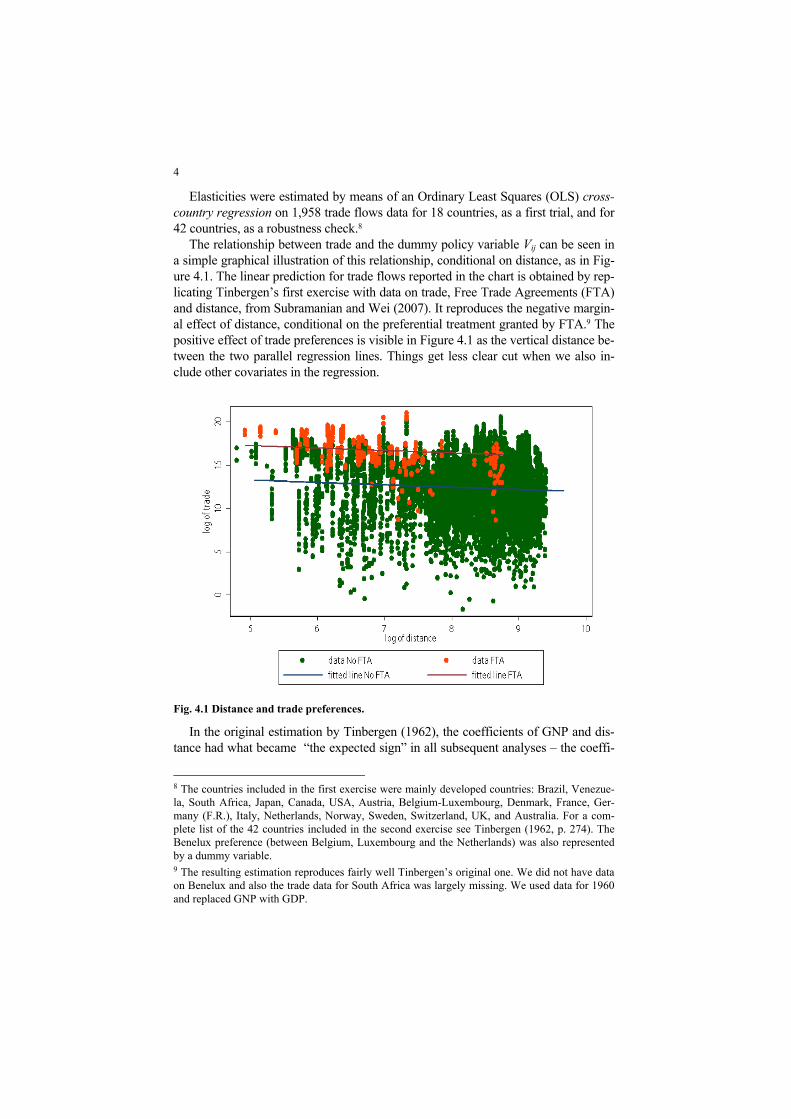
The relationship between trade and the dummy policy variable Vij can be seen in a simple graphical illustration of this relationship, conditional on distance, as in Fig-ure 4.1. The linear prediction for trade flows reported in the chart is obtained by rep-licating Tinbergen’s first exercise with data on trade, Free Trade Agreements (FTA) and distance, from Subramanian and Wei (2007). It reproduces the negative margin-al effect of distance, conditional on the preferential treatment granted by FTA.9 The positive effect of trade preferences is visible in Figure 4.1 as the vertical distance be-tween the two parallel regression lines. Things get less clear cut when we also in-clude other covariates in the regression.
Fig. 4.1 Distance and trade preferences.
In the original estimation by Tinbergen (1962), the coefficients of GNP and dis-tance had what became “the expected sign” in all subsequent analyses – the coeffi-
8 The countries included in the first exercise were mainly developed countries: Brazil, Venezue-la, South Africa, Japan, Canada, USA, Austria, Belgium-Luxembourg, Denmark, France, Ger-many (F.R.), Italy, Netherlands, Norway, Sweden, Switzerland, UK, and Australia. For a com-plete list of the 42 countries included in the second exercise see Tinbergen (1962, p. 274). The Benelux preference (between Belgium, Luxembourg and the Netherlands) was also represented by a dummy variable. 9 The resulting estimation reproduces fairly well Tinbergen’s original one. We did not have data on Benelux and also the trade data for South Africa was largely missing. We used data for 1960 and replaced GNP with GDP.
5
cients of the economic attractors were positive and the one of distance was negative – and resulted relevant and significant.10 Moreover, the fit of the estimation was found to increase when the data sample was increased from 18 to 42 countries; on the other hand, the coefficient for adjacency was never significant and the one for trade preference was borderline. Although its functioning wasn’t perfect, Tinbergen, who was a correlation hunter (Szenberg 1992, p. 278), succeeded in identifying a specification whose key variables explained a very high percentage of variability in the data, with a multiple correlation coefficient, R2, of 0.82. This result led the way to the application of the log-linearized version of Newton’s universal law of gravity to social interactions. Since then, the equation was viewed as a big success in en-lightening “… the dominant role played by … exporters’ and importers’ GNP and distance in explaining trade flows” (Tinbergen 1962, p. 266).
The specification however, left room for improvement, and the positive but rel-atively small role of trade preferences was an issue that stimulated further inquiry. In this chapter we will address some of the main open issues – associated to Tin-bergen’s original wording, that we have highlighted by marking the text in italics – one at a time. We will review, briefly, the theoretical and, more extensively, the empirical trade literature on the gravity equation and we will indicate some of the promising avenues for future research.
4.2 Estimating gravity
Let’s start from the first term highlighted in the introduction: determined. Bilateral trade flows are determined by the variables included in the right-hand-side of the gravity equation. This implies a clear direction of causality that runs from income and distance to trade. This direction of causality is however theory-driven and based on the assumption that the gravity equation is derived from an microeco-nomic model where income and tastes for differentiated products are given. Em-pirically, the causality (as if in a randomized quasi-experimental setting11 à la Ru-
10 In his comments to the regression’s functional form, Tinbergen explained that in his view the economic size (GNP) of the importing country played a twofold role: it indicates its demand – external and internal - and its degree of diversity of production. In principle, the sign of the coef-ficient could have been positive (demand) or negative (self-sufficiency). For Tinbergen it was a surprise that the coefficient was positive. It was also a surprise to observe that countries “trading less than normally” (below the regression line) were the bigger and the richer countries. Though the second evidence – small countries trade more with the rest of the world - has been explored theoretically (Anderson 2010) and empirically (Alesina et al. 2005; Rose 2007), the role played by self-sufficiency has been largely neglected by the literature. 11 In this setting researchers are interested in the causal effect of a treatment that takes the form of binary trade policy intervention (when the treatment is a dummy variable) or an ordered or continuous trade policy intervention (when considering trade preferential margins). Units, in this case countries or specific sectors of a country, are either exposed or not exposed to the treatment. Even if the effect of the treatment can be potentially heterogeneous across units, usually re-
6
bin) of the gravity equation, as described in equation 4.1, is more difficult to estab-lish: the equation as it stands represents a regression of endogenous variables on endogenous variables. As a consequence, the parameter of the gravitational con-stant G is not constant: it varies by trade partner and over time and is correlated with many, if not all, policy variables affecting trade (which are rarely considered as the equivalent of a treatment in a random trial experimental setting). Failure to acknowledge this leads to an estimated impact of the policy variables likely to be biased and often severely so.
We are in the realm of omitted variable biases. To simplify, let’s assume away GDPs and distance and focus on the policy variables. The estimated gravity equa-tion will have the following structure:
, , ,
0
5constant policy iid
ln lnij ij ij
a
X G a V H{
� �
(4.2)
while the true structural model is:
, , ,
0
5 6constant policy iidomitted varible
ln ln lnij ij ij ij
a
X G a V a Z H{
� � ����
. (4.3)
We can write Zij as a function of Vij in an auxiliary regression:
, , ,0 1
constant policy iid
ln ij ij ijZ b bV u � �
. (4.4)
Without being aware of it, we have estimated the following equation:
0 0 6 5 6 1 6
constant policy iid
ln ( ) ( ) ( )ij ij ij ijX a b a a a b V a uH � � � � � � � ���� ����� ���
. (4.5)
Therefore, unless b1=0, 5 5 6 2
bias
ˆE( ) ij ij
ij
v za a a
v
ª º � « »
« »¬ ¼
¦¦
�����
. Accordingly, the bias
depends on the correlation between the policy variable and the omitted variable, and can have a positive or negative sign. Furthermore, the mis-specification also affects the standard errors, which would result in a positive bias (Wooldridge, 2002, Chapter 4).
searchers focus on the identification of an average treatment effect (see Angrist and Pischke 2009 for a discussion of quasi-experimental settings).
7
The omitted variable problem in the gravity equation has been dealt through different approaches. The first has been to include in the equation one or more proxy variables correlated with the omitted variable. We will discuss this strategy in the context of the effect of distance on trade. A second approach has been to in-clude a time-dimension in the analysis and to move from cross-country analysis to panel data analysis, since one of the most likely sources of omitted variables is country heterogeneity, an issue that is not likely or easy to account for in a cross-country setting. While we will tackle the aspects related to a correct specification in the following example, where we show that the biases from mis-specification are non-trivial, here we would like to focus on the choice between cross-section and panel estimations. Even though elements such as distance and size are best captured by cross sections with the panel not adding much content in short hori-zons, in most cases panel specifications should be preferred to cross-section speci-fications because of the inability of the latter to properly account for the omitted variables bias. On the other hand, policy effects, such as the trade promotion of free trade agreements or custom unions, are always better identified in panels, through the time series dimension. Indeed, in the cross section specification they are highly collinear with distance.
With these issues in mind, in the next two sections we first empirically show the potential biases from a bad specification and then provide a synthetic discus-sion of how to specify a theoretically sound gravity equation. The aim is to give the reader an informed perspective of what theory-based specifications can be ap-plied to address the various empirical questions posed to the gravity equation.
4.2.1 How big are the biases?
In order to show how big are the biases from mis-specifying the gravity equation, we re-run Tinbergen’s regression as a benchmark, for the same subset of 42 coun-tries and for data taken at intervals of five years, from 1960 to 2005. We will show that the trade policy variable coefficient is very sensitive to the specification. In particular, we show the effect of introducing different types of fixed effect con-trols and of using real-vs-nominal GDP.12 Results are reported in Table 4.1 below.
12 The use of nominal GDP (instead of real GDP) is theoretically more sound. We will come back to this issue in Section 4.4.3.2.
8
Table 4.1 The Gravity equation with different fixed effects.
exporter and importer time invariant fe no no no no yes yes no no
exporter and importer time-varying fe no no no no no no yes yes
time invariant pair fe no no no no no no no yes
Note: robust standard errors in parentheses. (*) significant at 10% level; (**) significant at 5% level; (***) significant at 1% level.
Columns (1) and (2) report the base regression as in Tinbergen (1962), with on-ly two differences. First, instead of GNP we use GDP (in column (1) real GDP and in column (2) nominal GDP). Second, our policy variable of interest is wheth-er a country pair is in an FTA relationship. Columns (3) and (4) reports results where time dummies are added to the regression, to account for the changing na-ture of the relationship over time, with the difference between column (3) and (4)
9
being the real-vs-nominal GDP choice. Column (5) and (6) report results with time invariant importer and exporter fixed effects on top of the time dummies. Column (7) shows results for time varying exporter and importer fixed effects. Lastly, col-umn (8) presents a specification where time invariant pair effects are also added.
In spite of Figure 4.1, the baseline Tinbergen-like specification seems to sug-gest that being in an FTA does not have any statistically significant effect on trade if we use real GDP, but a positive and statistically robust effect if we use nominal GDP (columns 1 and 2). Similarly, adjacency (i.e. sharing a border) does not seem to be trade-enhancing when we use real GDP figures, and positive and significant when we use nominal GDP figures. All other variables have the expected sign and are statistically significant, with both GDP specifications. Adding time fixed ef-fects (columns 3 and 4) and time-invariant importer and exporter fixed effects (columns 5 and 6) however has the surprising effect of reversing the sign of the FTAs coefficient in three out of the four cases. Notwithstanding the sign of the coefficient, the fact that the FTA coefficient acquires statistical significance and that its point estimates increase with the inclusion of time dummies, suggests the existence of a significant time trend non-orthogonal to the FTA dummy. Interest-ingly, while the FTA coefficient is negative, the coefficient for sharing a border is positive and strongly significant. The two results in combination lead us to formu-late the hypothesis that the two variables might be correlated with each other. If this the case, entering the exporter and importer fixed effects in a time-varying way does not help achieving a sound specification.13 Hence the only solution re-mains changing slightly the focus of our research question, by asking, what is the effect of entering in a FTA relationship for bilateral trade? With this different an-gle, we can formulate a gravity specification where we add time invariant pair ef-fects on top of time-varying importer and exporter fixed effects to address pair-specific invariant omitted variables. The outcome is an FTA coefficient positively signed and statistically significant. The coefficient is now to be interpreted as the effect of entering in an FTA instead of being part of it, i.e. with this specification a country-pair that was part of a bilateral agreement throughout the period of obser-vation would not be picked up by the FTA dummy.14
Given the evidence of how important it is to properly specify the gravity equa-tion to account for country heterogeneity, we now turn to provide the reader with an informed perspective on the empirical issues associated with the estimation of the gravity equation. We do this by discussing how to achieve theoretically sound
13 Another source of bias in the regression could come from self-selection, i.e. nations that choose to be in a given trade policy regime are not randomly chosen. Geographical proximity, common language, common border, former colonial status, size and wealth of a nation are likely to strongly influence the decision to enter or not in given policy regimes. This causes a selection problem. Matching methods have been used to control for self-selection (see Persson (2001) for an early application and Millimet and Tchernis (2009) for a discussion of the methodology). However, solving for self-selection needs to be done on a case by case basis. 14 Fixed effects specifications require getting rid of RHS variables that are accounted for by the fixed effects. This explains why we have no entries for GDP, distance and border in columns (5) to (8).
10
gravity specifications. In other words, abandoning for a while Tinbergen’s word-ing, we link the gravity equation to the gravity model.
4.3 Theory-based specifications for the gravity model
For Tinbergen (1962, p. 263) the gravity equation was a “turnover relation”, where no separate demand and supply were considered, no prices were specified, and no dynamics was taken into account. This doesn’t mean that there was no model under the equation. The exporter’s and importer’s GNPs captured respec-tively the effect of production capacity and of demand and distance was a measure of the trade feasibility set. Assumptions were not spelled out and restrictions were not explicitly imposed, but a model was already in nuce. Surprisingly, all devel-opments up to the early 1980s concerned the empirics of the relationship, while the theoretical basis remained underdeveloped.15 Since then, things have changed radi-cally. Three decades of theoretical work has shown that the gravity equation can be derived from many different – and sometimes competing – trade frameworks. In 1979, James Anderson proposed a theoretical explanation of the gravity equation based on a demand function with constant elasticity of substitution (CES) à la Arm-ington (1969), where each country produces and sells goods on the international market that are differentiated from those produced in every other country. Later work has included the Armington structure of consumer preferences in (i) monopo-listic competition frameworks (Krugman 1980; Bergstrand 1985, 1989; Helpman and Krugman 1985), (ii) models à la Heckscher-Ohlin (Deardorff, 1998), or (iii) models à la Ricardo (Eaton and Kortum 2002). The catalyst of the more recent wave of theoretical contributions on gravity is the literature on models of interna-tional trade with firm heterogeneity, spearheaded by Bernard et al. (2003) and Me-litz (2003).
Given the plethora of models available, the emphasis is now on ensuring that any empirical test of the gravity equation is very well defined on theoretical grounds and that it can be linked to one of the available theoretical frameworks. Accordingly, the recent methodological contributions brought to the fore the im-portance of defining carefully the structural form of the gravity equation and the implications of mis-specifying equation (4.1). In this context, two broad sets of key issues have been identified. A first important range of contributions is related to the multilateral dimension of the gravity model. Anderson and van Wincoop (2003) – building on Anderson (1979) – showed that the flow of bilateral trade is influenced by both the trade obstacles that exist at the bilateral level (Bilateral Resistance) and by the relative weight of these obstacles with respect to all other countries (what they called the Multilateral Resistance). After this contribution, the omission of a
15 Alan Deardoff refers to the gravity model as having “somewhat dubious theoretical heritage” (Deardoff 1998, p. 503). Similar assessments can be found in Evenett and Keller, 2002 and Har-rigan, 2001.
11
Multilateral Resistance term is considered a serious source of bias and an important issue every researcher should deal with in estimating a gravity equation. The second main area of methodological concern is related to the selection bias associated to the presence of heterogeneous firms operating internationally. Contrary to what is implied by models of monopolistic competition à la Krugman, not all existing firms operate on international markets. In fact, only a minority of firms serves for-eign markets (Mayer and Ottaviano 2008; Bernard et al. 2007). Moreover, not all exporting firms export to all foreign markets as they are generally active only in a subset of countries.16 The critical implication of firm heterogeneity for modeling the gravity equation is that the matrix of bilateral trade flows is not full: many cells have a zero entry. This is the case at the aggregate level and the more often this case is seen, the greater the level of data disaggregation. The existence of trade flows which have a bilateral value equal to zero is full of implications for the gravity equation because it may signal a selection problem. If the zero entries are the result of the firm choice of not selling specific goods to specific markets (or its inability to do so), the standard OLS estimation of the gravity equation would be inappropriate: it would deliver biased results (Chaney 2008; Helpman et al. 2008).
Irrelevant of the theoretical framework of reference, most of the modern main-stream foundations of the gravity equation are variants of the demand-driven model described in the appendix of Anderson (1979). Hence, in the following par-agraphs, we summarise the key theoretical points of this common framework. We will mainly rely on the Anderson and van Wincoop (2003) and Baldwin and Ta-glioni (2006) derivations, using standard notation to facilitate the exposition. We will obviously mention where and in what way the supply-driven models à la Eaton and Kortum (2001) differ.
The starting point of Anderson and van Wincoop (2003) is a CES demand structure, with the assumption that each firm produces a unique variety of a unique good. Since trade data are collected in value terms it is convenient to work with the CES expenditure function rather than the CES demand function. The solution to the utility maximisation problem tells us that spending on an imported good that is produced in nation i and consumed in nation j is:
16 The heterogeneity in firm behaviour is due to fixed costs of entry which are market specific and higher for international markets than for the domestic market. Hence, only the most produc-tive firms are able to cover them. Firm productivity is furthermore correlated with a large array of other observable firm characteristics. Hence firms that serve both domestic and foreign mar-kets are not only more productive but also larger, more innovative and more intensive in human and physical capital. By contrast firms that only serve the domestic market are less productive, smaller, less innovative, and labour intensive.
12
where xij is the expenditure in destination country j on a variety made in country i, Pj is nations-j’s CES price index, V is the elasticity of substitution among varieties assumed greater than one, and Mj is nation-j expenditure, and pij is the consumer price in nation j of goods produced in nation i
ijiijij pp IP (4.7)
In this equality, pi is nation i’s domestic price, Pij is the bilateral price mark-up (which depends on the assumed market structure) and Iij is the bilateral “trade costs”, which is one plus the ad-valorem tariff equivalent of all natural and manmade barriers, i.e. whatever cost-factor that introduces a wedge between do-mestic and foreign goods’ prices, conditional on market structure. This is the pass-through equation. Combining this with equation (4.6) gives us the per-variety rela-tionship. Aggregating over all varieties exported from country i to country j (as-suming that all varieties produced in nation i are symmetric) yields aggregate bi-lateral trade:
� �1 1
jij ij ij ij i ij
i j
MX x n p
PV
VP I�
� ¦ (4.8)
where Xij indicates the value of the aggregate trade flows (measured in terms of the numeraire), and nij indicates the number of nation-i varieties sold in nation-j.17
Let us stress the point that our derivation of the gravity equation is based on an expenditure function. This explains two key factors. First, destination country’s GDP enters the gravity equation (as Mj) since it captures the standard income ef-fect in an expenditure function. Second, bilateral distance enters the gravity equa-tion since it proxies for bilateral trade costs which get passed through to consumer prices and thus dampens bilateral trade, other things being equal. The most im-portant insight from the above mathematical derivation is that the expenditure function depends on relative and not absolute prices. This allows factoring in firms’ competition in market j via the price index Pj. Hence, equation (4.8) tells us that the omission of the importing nation’s price index Pj from the original gravity equation described in equation (4.1) leads to a mis-specification. It should further be noted that the exclusion of dynamic considerations is problematic: Although we omitted time suffixes for the sake of simplicity, the reader should be aware that Pj is a time-variant variable, so it will not be properly controlled for if one uses time-invariant controls, unless the researcher is estimating cross-sectional data.
Having shown why destination-country GDP and bilateral distance enter the gravity equation, we turn next to explaining why the exporter’s GDP should also be included. The explanation is Tinbergen’s: it reflects the export capacity or the supply 17 Anderson and van Wincoop (2003, p. 174) assume that this number is equal to 1 for all origin and destination markets.
13
available on the side of the exporter. While the way it enters the equation is the same across theoretical frameworks, the interpretation of the role it plays depends on the specificities of the underlying theory. The Anderson-van Wincoop derivation is based on the Armington assumption of competitive trade in goods differentiated by country of origin. In other words, each country makes only one product, so all the adjustment takes place at the price level. This implies that nations with large GDPs export more of their product to all destinations, since their good is relatively cheap. This equates to saying that their good must be relatively cheap if they want to sell all the output produced under full employment. Helpman and Krugman (1985) make assumptions that prevent prices from adjusting (frictionless trade and factor price equalisation), so all the adjustment happens in the number of varieties that each na-tion has to offer. This implies that nations with large GDPs export more to all desti-nations, since they produce many varieties. Since each firm produces one variety and each variety is produced only by one firm, stating that the adjustment takes place at the level of varieties equates to stating that the number of firms in each country adjust endogenously. This is enough to lead to the standard gravity results.
Turning back to Anderson and van Wincoop and how the exporter’s GDP should enter the gravity equation, the idea is that nations with big GDPs must have low relative prices so to sell all their production (market clearing condition). To determine the price pi that will clear the market, we sum up nation i’s sales over all markets, including its own market, as Tinbergen originally pointed out (Tin-bergen, 1962, pp. 60-61) and set it equal to overall production. This can be written as follows:
i ij ijj
M n x ¦ which equates to � �111
ji i ij ij ij
j j
MM p n
PVV
VP I��
�
ª º « »
« »¬ ¼¦ ,(4.9)
where the second equality follows from the substitution of the expression for xij, that is produced in turn by the substitution of equation (4.7) into equation (4.6). Solving equation (4.9) for 1
ip V� yields:
1 ii
i
Mp V�
: where � �¦
»»¼
º
««¬
ª : �
�
j j
jijijiji P
Mn V
VIP 11 4.10)
where :i represents the average of all importers’ market demand – weighted by trade costs. It has been named in many different ways in the literature, including market potential (Head and Mayer 2004, Helpman et al. 2008), market openness (Anderson and van Wincoop 2003) or remoteness (Baier and Bergstrand 2009).
Using equation (4.10) in equation (4.8) yields a basic but correctly specified gravity equation
� �1 1
j iij ij ij ij
j i
M MX n
PV
VP I�
� :
(4.11)
14
If we suppose that each country only produces one product, as in Anderson and Van Wincoop (2003), i.e. nij (=1), and assume that the markup ȝij depends upon the distance between the two trading partners, we arrive to the most familiar speci-fication of the gravity equation:
i
i
j
jijij
MPM
X:
��
VVI 1
1
(4.12)
Hence, we just showed that origin country’s GDP enters the gravity equation since large economies offer goods that are either relatively competitive or abun-dant in variety, or both. The derivation also shows that the exporting nation’s market potential i: matters, and that the misspecification in the gravity equation would be more serious the bigger the asymmetry among countries.
Equation (4.12) is identical to equation (4.9) in Anderson and van Wincoop (2003, p. 175). But it is not identical to their final expression. As shown by Bald-win and Taglioni (2006), Anderson and van Wincoop (2003) assume that
V� : 1ii P for all nations, since it is a solution to the system of equation that de-
fines these two terms. There are three critical assumptions behind this. First, they assume that trade costs are two-way symmetric across all pairs of countries. This assumption however is automatically violated in the case of preferential trade agreements. Second, they assume that trade is balanced, i.e. Xij = Xji, also an hy-pothesis that is often violated in practice. Finally, they assume that there is only one period of data. Were the above three conditions verified, we could refer to the product of the two terms i: and V�1
iP as to a single country geography index, with the well known term of multilateral resistance; which can be empirically controlled for by a time-invariant country-fixed effect.18 In fact, a more general case is that i: and V�1
iP are proportional, i.e. that 1i iP VD �: and that there is a
different Į per year. If this point is acknowledged, it is simple to see that the gravi-ty model in equation (4.1) is missing a time-varying dimension and that i: and
V�1iP must be accounted for with separate terms. An easy and practical solution to
match the theory with the data is to introduce time-varying importer and exporter fixed effects. Obviously, in cross-sections, the Anderson van Wincoop specifica-tion is sufficient owing to the lack of time dimension. Often however, the need of correcting for omitted variables biases clashes with problems of collinearity with
18 Obviously, some econometric fixes have been found. In particular, the practice introduced by Harrigan (2001) and popularized by Feenstra (2003), to control for Multilateral Resistance through the use of country fixed effects in the econometric estimation. Incidentally, the country fixed effect practice diverted the analysis from the causes of multilateral resistance to the effects of multilateral resistance. The latter remains a promising area of analysis, especially in the con-text of policy evaluation.
15
the other variables. Hierarchical Bayesian methods may be able to assist in reduc-ing the resulting overparametrization problem (Guo 2009), but not in solving it. Alternatively, more sophisticated terms that account for i: and V�1
iP but that are orthogonal to the other variables in the equation must be computed, or strategies to control for potential collinearity have to be devised case-by-case.
A final aspect to consider is firm heterogeneity and the connected issue of ze-roes in the trade matrix. In models with identical firms, in the absence of natural and man-made trade costs, countries either trade or they are in autarky. If they do trade, every firm in a country exports to every country in the world. Introducing firm heterogeneity in models of international trade however allows for a more re-alistic representation of reality, namely one where not all firms in a country ex-port, not all products are exported to all destinations and not all countries in the rest of the world are necessarily served. Moreover, as trade barriers move around, the set of exporters will change, and this additional margin of adjustment – the ex-tensive margin – will radically change the aggregate trade response to the under-lying geographical and policy variables. Helpman et al. (2008), from a demand side, and Chaney (2008), from a supply side, have both introduced heterogeneity in gravity models, allowing for the more general derivation of gravity with heter-ogeneous firms.
Consider a world with many countries and same CES preferences across coun-tries with elasticity of substitution ı>1. Country i has a given number Ni of poten-tial producers, i.e. entrants. These entrants draw their unit input requirement a from a distribution G(a) = (a/Ɨ)k, where k > ı-1 and 0 � a � Ɨ. The term k denotes the productivity distribution parameter that governs the entry and exit of firms into the export markets. Hence k indicates the degree of firm heterogeneity and ı the degree of differentiation across products. The same distribution G(a) holds across countries, but the cost of the input bundle wi is country-specific. Trade costs Iij for trade between countries i and j are composed of a variable and a fixed part. The variable component is IJij�1, a per-unit iceberg trade cost. The fixed component is fij>0 . These costs include also serving the domestic market where i = j and where one can assume that IJii = 1 and that fij includes overhead fixed costs.
If a producer in country i with unit cost a exports to j, it will set a price pij(a) and generate export sales xij(a) and export profits ʌij(a):
awap ijiij W
VV
1)(
�
(4.13)
VV
�� 1
1 )()( apPM
ax ijj
jij
(4.14)
16
ijiijij fwaxa � )(1)(
VS
(4.15)
As before jM and V�1jP are expenditure and price index respectively in im-
porter country j. The cut-off for profitable exports from i to j which we define aij is determined by ʌij(aij) = 0. In other words, we assume that Ɨ is high enough to allow that a�Ɨ for every pair of countries i and j.
Given this, aggregate bilateral trade from i to j is then
³ ija
ijiij adGaxNX0
)()( (4.16)
If one defines ¦ j
iji XM as the value of country i´s aggregate output,
where trade with every country in the world including self is accounted for, then – after some algebraic transformations – the aggregate bilateral trade from i to j can be written as follows:
The gravity specification with firm-heterogeneity differs from previous specifi-cations in two broad ways, which we summarise below. While some of the points we will make are already clear from equation (4.17), the interested reader is re-ferred to Chaney (2008) which demonstrates explicitly each of the issues that we raise below. He does so by decomposing equation (4.17) by the two margins of trade, solving for each expression and expressing each margin in elasticities.
To start with, the per-unit trade costs are shown to affect both the intensive and the extensive margin of trade. However, they do so with some important differ-ences. First, per-unit trade costs IJij are subject to firm heterogeneity (as indicated by the superscript k) and no longer to product differentiation (i.e. the parameter 1-V in equation 4.12). This is due to the fact that, with Pareto or Frechet distributed productivity shocks, the effect of V on the intensive and extensive margin cancels out, so that in aggregate the elasticity of trade flows with respect to the per-unit trade costs only depends on k. Nevertheless, when per-unit trade costs move, both the intensive and the extensive margin of trade are affected and ı, the degree of
17
competition in the market, plays an important role in the dynamics. The intensive margin of trade responds to changes in variable trade costs as in traditional speci-fications: i.e. the elasticity of incumbent exporters with respect to IJij is (ı-1), hence each firm faces a constant elasticity residual demand, and therefore when goods are very substitutable, the export of incumbents is very sensitive to trade costs. The extensive margin, on the other hand, behaves idiosyncratically. When per-unit trade costs move, some of the less productive firms start exporting, but their im-pact on aggregate flows is inversely proportional to ı. As goods become more substitutable (high ı), the market share of the least productive firms shrinks com-pared to the market share of the more productive firms and the change in trade costs has a decreasing impact on aggregate trade flows. Finally, fixed costs only matter for the extensive margin of trade, since those exporters that have already decided to enter a market are not going to change their decision. This effect is clearly visible with a first order approximation, as the derivative of trade flows to fixed costs posts zero elasticity for the intensive margin. A second important set of implications of firm-heterogeneity for gravity models arises because the importer CES market demand effect is amplified by the upshot of demand on the extensive margin of trade k/(ı – 1)>1. By contrast, the exporter’s market potential is com-puted as in previous models, given however differences in trade costs and the ex-istence of importer fixed effects. Having shown how to handle firm heterogeneity in gravity models from a theoretical point of view,19 in the following sections of the chapter we will now come back to Tinbergen’s wording and discuss the empir-ical strategies that allow making use of the information contained in the trade model founding the gravity equation.
4.4 A piecewise analysis of the gravity equation
4.4.1 Dependent variable
To put things in context, there are three issues associated with the left-hand side variable of the gravity equation. The first has to do with the issue of conversion of trade values denominated in domestic currencies and with the issue of deflating the time series of trade flows. The second is associated with the effect of the inclu-sion or exclusion of zero-trade flows from the estimation. Finally, the third issue is related with the typology of goods or economic activities to be included in the def-
19 From a practical point of view, it is not necessary to rely on firm-level data to consider the ef-fect of firms heterogeneity. Given the productivity distribution of domestic firms, the aggregate volume of trade defines the volume of trade of the marginal exporting firm – the one with the productivity exactly equal to the cut-off point of the productivity distribution.
18
inition of trade flows: imports, exports, merchandise trade or any other possible candidate for a trade link between country i and country j. In the current section we will discuss the third and the first issues while leaving the problem of zero-trade flows for a more focused discussion in Section 4.5.1.
Starting with the issue of typology, in the large majority of studies the depend-ent variable is usually a measure of bilateral merchandise trade.20 Three choices of trade flow measures are available to the researcher for the dependent variable of a classical gravity equation on goods trade: export flows, import flows or average bilateral trade flows. The choice of which measure to select should be driven first and foremost by theoretical considerations which mostly imply privileging the use of unidirectional import or export data. Sometimes however, considerations linked to data availability or differences in the reliability between exports and imports da-ta may prevail. For example, a common fix to poor data is to average bilateral trade flows in order to improve point estimates. This is done because averaging flows takes care of three potential problems simultaneously: systematic under re-porting of trade flows by some countries, outliers and missing observations. Alt-hough there are better ways of dealing with those problems,21 it is common prac-tice to justify the use of this procedure using the above arguments. This notwithstanding, caution should be applied in averaging bilateral trade. First of all, averaging is not possible in those cases where the direction of the flow is an im-portant piece of information. Second, if carried out wrongly, averaging leads to mistakes.
Average bilateral trade is constructed by averaging the exports of country i to country j with the exports of country j to country i. Since each trade flow is ob-served as exports by the origin nation and imports by the destination country and most countries do both import and export from the same trade partner, typically four values are averaged to get the undirected bilateral trade that then needs to be log-linearised:22
20 Nevertheless, gravity models have also been employed for examining the determinants of trade in goods and services, other than merchandise. The gravity model offers a high probability of a good fit, but what we mentioned for trade in merchandise is also true for all other left-hand side variables: there is no reliable gravity equation without a supporting theoretical model. If one wants to explore a gravity model on FDI, it is better to have a theory to refer to (as in Carr et al. 2001, or in Baltagi et al. 2007). The need for a theory is even more compelling if one wants to account for the many alternative strategies that heterogeneous firms have at their disposal to serve foreign markets, i.e. trade and FDI (and even differentiating further between offshoring or joint-ventures). 21 It is true that reliability of the data varies significantly from country to country. But if this cor-responds to a national characteristic that is considered to be constant along time, the country-specific quality of the data can be controlled for, as any other time-invariant country characteris-tic or country fixed effects. 22 In constructing average trade, the researcher should make sure that the observations are statis-tically independent. Hence, if the two trade partners import and export from each other caution should be taken to cluster the four single observations in one single data point. We will come back to the issue of independence latter on.
19
E( , , , )ij ij ji ij jiT x x m m
(4.18)
A bias may arise if researchers employ the log of the sum of bilateral trade as the left-hand side variable instead of the sum of the logs.23 Many published studies in the field of trade analysis, including some very recently published works, carry this bias. The mistake will create no bias if bilateral trade is balanced. However, if nations in the treatment group (i.e. the countries exposed to the policy treatment which average effect is being estimated) tend to have larger than usual bilateral imbalances – this is the case for trade between EU countries and also for North-South trade – then the misspecification leads to an upward bias of the treatment variable. The point is that the log of the sum (wrong procedure) overestimates the sum of the log (correct procedure). This leads to an overestimated treatment varia-ble, as shown in Baldwin and Taglioni (2006). At any rate, the mistake implies that the researcher is working with overestimated trade flows within the sample.
Turning to conversion, the first item listed at the beginning of the section, trade should enter the estimation in nominal terms and it should be expressed in a com-mon numeraire. This stems from the fact that the gravity equation is a modified expenditure equation. Hence, trade data should not be deflated by a price index. Deflating trade flows by price indices not only is wrong on theoretical grounds but it also leads to empirical complications and likely shortcomings, due to the scant availability of appropriate deflators. It is practically impossible to get good price indices for bilateral trade flows, even at an aggregate level. Therefore, approxima-tions may become additional sources of spurious or biased estimation. For exam-ple, if there is a correlation between the inappropriate trade deflator and any of the right-hand side variables (the trade policy measures of interest), the coefficient will be biased, unless the measures are orthogonal to the deflators used.
As far as accounting conventions are concerned, trade data can be recorded ei-ther free on board (FOB) or gross, i.e. augmented with the cost of insurance and freight (CIF).24 Using CIF data may lead to simultaneous equation biases, as the
23 Since the gravity equation is mostly estimated in logs, the practice of averaging trade flows of-ten results in using the log of the sum of the flows instead of the sum of the logs. 24 Most common sources of trade data include the following. International Monetary Fund (IMF) DOT statistics (http://www2.imfstatistics.org/DOT/ ) provides bilateral goods trade flows in US dollar values, at annual and monthly frequency. UN Comtrade (http://comtrade.un.org/ ) provides bilateral goods trade flows in US dollar value and quantity, at annual frequency and broken down by commodities according to various classifications (BEC, HS, SITC) and up to a relatively dis-aggregated level (up to 5 digit disaggregation). The CEPII offers two datasets CHELEM (http://www.cepii.fr/ anglaisgraph/bdd/chelem.htm) and BACI (http://www.cepii.fr/anglaisgraph/bdd/baci.htm) which use UN Comtrade data but fill gaps. corrects for data incongruencies and CIF/FOB issues by means of mirror statistics. WITS by the World Bank provides joint access to UN Comtrade and data tariff lines collected by the WTO and ITC. The most timely annual, quarterly and monthly data are available from the WTO Statistics Por-tal. Similarly, the CPB provides data for a subset of world countries at the monthly, quarterly and annual frequency as indices. Series for values, volumes and prices are provided along with series for industrial production. Finally, regional or national datasets provide usually more detail. No-
20
dependent variable includes costs that are correlated with the right hand side vari-ables for distance and other trade costs. If FOB data are not available, ‘mirror techniques’, matching FOB values reported by exporting countries to CIF values reported by importing countries, can be used. These techniques however, remain to a large extent unsatisfactory due to large measurement errors (Hummels and Lugovskyy 2006). Hence, the suggestion as to this point is to be aware of whether CIF or FOB data are being used and interpret the results accordingly. If moreover the researcher is constructing a multi-country dataset, she should care for choosing data that are uniform, i.e. either all CIF or all FOB, controlling for measurement errors.
4.4.2 Covariates
As indicated above, a well specified gravity equation should include the “un-constant” terms i: and 1
jP V� . While several attempts at explicitly accounting for
these terms have been made, including by means of structural assumptions on the underlying model and the use of non-linear methods of estimations, the practice has increasingly moved towards the use of simple-to-use fixed effects for these terms. As discussed earlier, however, fixed effects methods sometimes cannot be applied due to problems of overparametrization and correlation with the variable of interest.
4.4.2.1 Fixed effects specifications
The advantage of using fixed effect specifications lies in the fact that they repre-sent by far the simplest solution to testing a gravity equation: they allow using OLS econometrics and do not require imposing ad-hoc structural assumptions on the underlying model. Specifications that make use of fixed effects are also very parsimonious in data needs: they only require data for the dependent variable and good bilateral values to estimate trade friction ijI .
Some caution however should be applied when using fixed effects on panel da-ta. Importer and exporter fixed effects should be time-varying, as they capture time varying features of the exporter and importer, as discussed in the theory sec-tion above. Similarly, if data are disaggregated by industry, country-industry spe-
table examples are the US and EUROSTAT (EU27) bilateral trade data available in values and quantities up to the 10-digit and 8-digit level of disaggregation respectively. Australia, New Zea-land and USA also collect consistent CIF and FOB values at disaggregate levels of bilateral trade. Interesting is also the case of China, It is interesting to note that China, besides providing SITC classifications also provides data series for processing trade.
21
cific time-varying fixed effects should be applied. With very large panels, this may lead to computational issues. Whatever the solution the researcher devises, it is a necessary condition to control for the omitted time-varying terms i: and
1jP V� and to avoid large biases on the estimates of the other explanatory variables.
Therefore, if computational complications arise, the researcher is recommended to find a way to solve the computational issues rather than giving up on properly specifying fixed effects. One final note of caution is in order: the use of exporter and importer fixed effects is suitable only if the variable of interest is dyadic, i.e. for ijI . If by contrast, the latter is exporter or importer specific, exporter and im-
porter specific variables should be introduced explicitly and other means of avoid-ing the omitted variables bias (i.e. of controlling for i: and 1
jP V� ) should be de-
vised. Finally, pair (exporter-importer) fixed effects can also be used, if appropriate and if their introduction does not generate problems of collinearity with other explanatory variables.
4.4.2.2 Attractors
In line with the theoretical specification, attractors should reflect expenditure in the country of destination and supply in the country of origin. GDP, GNP and Population are all measures that have been used as proxies of the above terms. Per capita GDP (Frankel 1997) and measures for infrastructural development (Limao and Venables 2001) have also been used. Again, the appropriate measure should be selected on the basis of theoretical considerations.25 As in the case of the de-pendent variable, these measures should enter in nominal terms. At any rate, de-flating them would have no impact if one includes time fixed effects, which would swipe them away.
Many studies, the large part of them in a cross-sectional setting, augment the gravity equation with variables that could ease trade relations. Sharing a common language, common historical events – such as colonial links, common military al-liances or co-membership in a political entity –, common institutions or legal sys-tems, common religion, common ethnicity or nationality (through migration), sim-ilar tastes and technology, and input-output linkages enhance international trade. Many of those issues are of interest per se and are worth to be explored. An ex-ample in point is Head et al. (2010) who, while examining the effect over time of the independence of post-colonial trade between the colonized country and the 25 This is true not only for variables to be included but also for restrictions on coefficients. From equation (4.14) the coefficient of Mi and Mj must be constrained to be one (this is why Anderson
and van Wincoop (2003) estimated the gravity equation using ij
i j
X
M M�as the left-hand side var-
iable). With heterogeneous firm, as in equation (4.17), this is not required.
22
former colonizer, conclude that trade flows are associated to some sort of relation-al capital that deteriorates with time if it is not renewed. They do so by showing that on average there is little short-run effect of the change in colony-colonizer re-lationship on trade: the reduction takes place progressively, over time, but trade does not stop suddenly, even in cases of hostile separation.
The researcher should be aware that most attractors have in general very low time variability. For this reason the researcher should pay particular caution in in-troducing them in fixed effects specifications. Should a specific attractor represent the core of the analysis, a safer option would be to avoid fixed effects estimations. This can be done by introducing measures of the exporter’s market openness i:
and importer’s CES price index, 1jP V� along with the trade partners’ GDPs. How-
ever, exporter’s market openness and, even more so, importer’s CES price index are difficult to construct. Once more, case-by-case solutions may be needed .26
4.4.2.3 Trade frictions
Distance matters! As Waldo Tobler’s first law of geography states: “Everything is related to everything else, but near things are more related than distant things.“ The question is why. As we emphasized in the introduction, Tinbergen’s idea is that physical distance is a rough measure of transportation or information costs about foreign markets - already too many things for one single rough (and robust!) measure. Econometric estimates of the constant elasticity of trade to distance range within an interval of –0.7 and –1.2 (Disdier and Head 2008) and distance appears to be very persistent over time (Brun et al. 2005).
In the early years of the empirical analysis on bilateral trade flows, many re-searchers focused on producing better approximations for trade distance than sim-ple Euclidean distance between the two poles of economic attraction of the two trade partners (respective capitals, main city in term of population or local produc-tion, main port or airport). To do so, some choose to estimate wedges between CIF and FOB data. Others used great-circle or orthodromic formulas.27 Nowadays, all most common distance measures across virtually all country pairs in the world are
26 It is difficult to give further details here, as the solutions should be devised case by case, based on the nature of the data at hand and on the research question. Nevertheless, options include in-troducing fixed effects at a different frequency than the attractors (Ruiz and Villarubia 2008; De Benedictis and Vicarelli 2009; Cardamone, 2011) or to only look at entries and exits in a differ-ent (policy) regime as we have done in section 4.2.1. 27 The great-circle, or orthodromic, formula is the formula used for calculating the distance be-tween longitude-latitude coordinates of the polar city of two countries is based on the spherical law of cosines is: cos (sin( ) sin( ) cos( ) cos( ) cos( - ))2a lat lat lat lat long long Rij i j i j iI � � � � � ;
where R= 6371 is the radius of the earth, in km.
23
freely available online28 or can be obtained from the applets of the most important geo-representations available on the web. The issue is therefore not anymore how to calculate physical distance between two countries in the most appropriate way, but how to interpret the distance coefficient and if distance has a linear effect on trade.
Starting from the second issue, there is no reason to believe that distance should be related to trade in a linear manner. Trade costs are much dependent on the characteristics of specific goods, such as fragility, perishability, size or weight. In aggregate terms, trade cost would be country specific, depending on country’s remoteness and sectoral specialization. In the absence of hard theoretical priors it is better to be agnostic and let the data speak. This is what has been done by Hen-derson and Millimet (2008). Using nonparametric techniques they found that the linearity assumption was supported by the data. We interpret this result as being clear evidence of variable trade costs being linear in distance for the average coun-try. But what about fixed costs?
From the literature on heterogeneous firms and trade we know that fixed costs affect only the extensive margin of trade (Chaney 2008). Lawless (2010), extends the strategy proposed by Bernard et al. (2007), and decomposes the dependent var-iable of the gravity equation (export flows to each different foreign market) into the number of firms exporting (the extensive margin) and average export sales per firm (the intensive margin). Although the proxy chosen for the intensive margin is not ideal in representing firm heterogeneity in exports, Lawless shows that dis-tance has a negative effect on both margins, but the magnitude of the effect is con-siderably larger and significant for the extensive margin. Furthermore, the varia-bles capturing the fixed cost (i.e. language, internal orography, infrastructure and import barriers) work through the extensive margin. Even Tinbergen (1962), in formulating the gravity equation as in (4.1) distinguished between variable costs (distance) and fixed costs. He approximated fixed costs by the cost-reducing effect of the adjacency dummy. We are therefore back to square one to the question of what lies behind the distance coefficient.
Let’s tackle this issue from a very general point of view. In modern economet-ric terms, the concept of distance as a rough measure of trade costs (broadly de-fined as every cost that generates a conditional wedge between domestic and for-eign prices) can be translated in the presence of a measurement error in the distance variable. It is well known that a measurement error in an explanatory var-iable, such as Iij , does result in a bias in the OLS estimates of a3 in equation (4.1).
Following on that, we can write the measured value of Iij as the sum of the true unobserved value of the trade cost Iij
* plus a measurement error eij that is an i.i.d. normally distributed random variable:
28 Cepii generated a positive externality for all researchers by making freely available their measures of distance (see http://www.cepii.fr/anglaisgraph/bdd/distances.htm). Jon Haveman, Vernon Henderson and Andrew Rose were pioneers in this matter. Haveman’s collection of In-ternational Trade Data and his “Useful Gravity Model Data” can be freely downloaded from, the F.R.E.I.T. database http://www.freit.org/TradeResources/TradeData.html#Gravity .
Consider now a simplified version of the gravity equation described in (1), where trade flows depend only on distance:
*
3 3 3ln ( )ij ij ij ij ij ijX a a a eI H I H � � � �. (4.20)
The presence of eij in the error term generates a mechanical correlation between the error term, 3( )ij ija eH � � , and the explanatory variable *
ij ij ijeI I � . It can
be shown (Wooldridge 2002, p. 75) that 3a converges in probability to a frac-
tion*var( )
1*var( ) var( )
ij
eij ij
I
I�
�of the true a3. This bias is called attenuation bias, since
3a is biased towards zero, irrespectively of whether a3 is positive or negative. The magnitude of the attenuation bias is linked to the so called signal-to-noise ratio
since *var( )ijI is the variance of the correct signal while var( )eij is the variance of
the noise. The larger the latter relative to the former, the larger is the magnitude of the attenuation bias, i.e. if half the variance of var( )ijI is noise, the bias would be
50%.29 If the distance variable is measured with error, we should expect an attenuation
bias in the relevant coefficient. There is a general consensus that the distance coef-ficient is instead too high and the fact that it is highly persistent and also increas-ing over time (Disdier and Head 2008) is at odds with the evidence reported by Hummels and Lugovskyy (2006) of a decreasing pattern in freight costs. Many have offered possible explanations; we will point out to a simple mechanical one. If the error-in-variable is not of the classical kind but is instead positively correlat-ed with the distance variable Iij, the bias would tend to be positive and the magni-tude would still depend on the signal-to-noise ratio.
Many authors have implicitly worked on the minimization of the signal-to-noise ratio, better defining the relevant meaning of “distance”. Some worked along the lines of distance as a proxy for transport costs, and it is surprising to ob-serve (Anderson and van Wincoop 2004) how little is known on transport costs
29 It is worth noting that in a multivariate regression we do not have such a clear and simple re-sult, but the bias will also depend on the correlation between Iij (measured with error) and other covariates. The problem is even more serious with estimates in first-differences, whose aim is to eliminate a possibly omitted fixed effect (Griliches and Haussman 1986). The traditional solution is to find an instrument correlated with distance but not with the error term.
25
and their different modes, their magnitude and evolution, and their determinants. Hummels and Skiba (2004) focus on the implications of differences in transport costs across goods on trade patterns, challenging the conventional Samulson’s iceberg assumption that transport costs are linear in distance. They show that actu-al transport costs are much closer to being per unit than iceberg, and they derive clear implications for trade: imports from more distant locations will have dispro-portionately higher FOB prices. Harrigan (2010) separates air and surface transport costs. Using a Ricardian model with a continuum of goods which vary by weight and hence transport cost, he shows that comparative advantage depends on relative air and surface transport costs across countries and goods. He tests the implication that the US should import heavier goods from nearby countries, and lighter goods from faraway countries, using detailed data on US imports from 1990 to 2003. Looking across US imported goods, nearby exporters have lower market share in goods that the rest of the world ships by air. Looking across ex-porters for individual goods, distance from the US is associated with much higher import unit values. The effects are significant and economically relevant. Jacks, Meissner and Novy (2008) work in the opposite direction, deriving distance measures from a Anderson-van Wincoop type gravity equation,30 and finding that the decline in this inherent measure of trade cost explain roughly 55 percent of the pre–World War I trade boom and 33 percent of the post–World War II trade boom, while the rise in that very measure explains the entire interwar trade bust. This stream of research requires a leap of faith on the data-generating process of the trade cost measure and the acceptance that trade costs are the trade empirics equivalent of the Solow’s residual: a measure of our ignorance.
Others have worked on Tinbergen’s idea that distance could be more than transport costs, moving from spatial distance to economic distance. In analogy with the inclusion of further attractors as explanatory variables, the gravity equa-tion has been therefore augmented with many dyadic variables that could reduce trade (trade policy aside). These variables are mainly associated with a common history of conflict, and are generally found to be highly significant (Martin et al. 2008a, 2008b).
The border between two nations is an equilibrium concept. It is the remaining evidence of the solution of a bargaining process concluding an international con-flict and is the fossil of historical events. Since the seminal works of McCallum (1995) and Helliwell (1996), trade economists have wondered how borders could generate a home bias in consumption. Using data on interprovincial and interna-tional trade by Canadian provinces for the period 1988-1990, McCallum (1995) showed that, other things being equal, the estimated interprovincial trade was more than 20 times larger than trade between Canadian provinces and US states. The result was striking and largely unbelievable. Anderson and van Wincoop (2003), controlling for multilateral resistance, reduced the border effect by half. Wei (1996), developing a procedure to calculate a country's trade with self – a measure rarely reported by official statistics, and relevant on a theoretical basis 30 See also Novy (2010) for a distance measure derived from heterogeneous firms trade models.
26
(being part of the consumer expenditure) – obtained the same reduction for OECD countries and much more for European countries. His estimate of the ratio of im-ports from self to imports from other European countries was 1.7. But he was not controlling for multilateral resistance and was using aggregate data. Disregarding the role of sectoral specialization would attenuate the border effect. Head and Mayer (2000) found that in 1985, Europeans purchased 14 times more from do-mestic producers (for the average industry) than from equally distant foreign ones. The border effect varies from sector to sector and is related more to consumer tastes than to trade barriers.
We would like to conclude this section on distance by mentioning that over the years, the gravity equation has been applied with great success also to issues which are only marginally related to the cost of physical distance. Blum and Gold-farb (2006) show that gravity holds even in the case of digital goods consumed over the Internet and that do not have trading costs. This implies that trade costs cannot be fully accounted by the effects of distance on trade.31 Using bilateral for-eign direct investment (FDI) data, Daude and Stein (2007) find that differences in time zones have a negative and significant effect on the location of FDI. They also find a negative effect on trade, but this effect is smaller than that on FDI. Finally, the impact of the time zone effect has increased over time, suggesting that it is not likely to vanish with the introduction of new information technologies. Portes and Rey (2005) show that a gravity equation explains international transactions in fi-nancial assets at least as well as goods trade transactions. In their analysis, dis-tance proxies some information costs, information transmission, an information asymmetry between domestic and foreign investors. Tinbergen would have been happy to know it, since he proposed information as a possible further explanation of the role of distance (Tinbergen 1962, p. 263). Guiso et al. (2009) go even fur-ther, finding that lower bilateral trust leads to less trade between two countries, less portfolio investment, and less FDI. The effect strengthens as more trust-intensive goods are exchanged.
4.4.2.4 Trade policy
As we pointed out in the introduction, the original use of the gravity equation by Tinbergen was ‘to determine the normal or standard pattern of international trade that would prevail in the absence of trade impediments’, which resulted in the evalu-ation of the effect of the British Commonwealth and of other FTA. The wider use of the gravity equation has still remained the same: the ex-post evaluation of the trade-enhancing effect of preferential trade policy.
31 Blum and Goldfarb (2006) also show that Americans are more likely to visit websites from nearby countries, even controlling for language, income, and immigrant stock. For taste-dependent digital products, such as music, games, and pornography, a 1% increase in physical distance reduces website visits by 3.25%. On the contrary, for non-taste-dependent products, such as software, distance has no statistical effect.
27
The mainstream approach to preferential trade policy evaluation still follows Tinbergen’s original strategy, defining the presence of FTA or Custom Unions (CU) or any specific preferential trade policy regime (i.e. Generalised System of Preferences (GSP), African, Caribbean and Pacific (ACP) Partnership, Everything But Arms (EBA), in the case of the European Union (EU)) with positive realiza-tion of a Bernoully process. In all these cases, as in Figure 4.1, the trade effect of the preferential trade policy is the marginal effect of a dummy variable that takes the value of one if the preferential trade policy affects the imports of country i from country j (in sector s at time t). The advantage of this strategy is in the ease of implementation. The list of existing FTA, CU, or specific preferential trade pol-icies is generally available online32 and subsets are included in many datasets used and made available by experts in the field.33 The disadvantages are that the dum-my identification for policy measures implies that all countries included in a treat-ed group are assumed to be subject to the same dose of treatment, which may be correct in the case of non discriminatory policy (e.g. the Most Favourite Nation (MFN) clause of the GATT/WTO agreement) but which is false in the case of non reciprocal preferential agreements. In addition, the treatment gets confounded with any other event that is specific to the country-pair and contemporaneous to the treatment (De Benedictis and Vicarelli 2009). Moreover, questions related to the effect of a gradual liberalization in trade policies cannot be answered using dum-mies, and the trade elasticity to trade policy changes cannot be estimated. Since this is the most common event (trade policy non facit saltus, at least not all the times shifts from zero to one) the use of a dummy for preferential trade policy can be a relevant shortcoming.
An alternative exists, and it is largely explored in this volume. It consists in switching from a dummies strategy to a continuous variables strategy, quantifying the preferential margin that the preferential agreement guarantees. This alternative strategy has been fruitfully used by Francois et al. (2006), Cardamone (2007) and Cipollina and Salvatici (2010). It opens an interesting research agenda and also of-fers some methodological challenges and some puzzling results.34 These issues will be discussed at length in Cipollina and Salvatici (2011).
Some issues are however worth discussing also in this context. The first is re-lated to the choice of the dependent variable and its consequences. Generally, the stream of literature adopting a dummy strategy focuses on aggregate effects, uses 32 The WTO collects all Trade Agreements that have either been notified, or for which an early announcement has been made, to the WTO (http://rtais.wto.org/UI/PublicMaintainRTAHome.aspx). The World Bank - Dartmouth College Tuck Trade Agreements Database can also be consulted at http://www.dartmouth.edu/~tradedb/trade_database.html 33 Andrew Rose’s homepage (http://faculty.haas.berkeley.edu/arose/RecRes.htm) is a great example of data sharing. It has encouraged new research and promoted the good practice of replicability in empirical research. 34 Francois et al. (2006) estimate of the trade policy elasticity has a huge variance and also in-clude some negative cases. This result is by no means exclusive to this stream of literature. Also some dummy strategy papers find negative coefficients to preferential dummies (Martínez-Zarzoso et al. 2009).
28
aggregated data, while all papers adopting the alternative strategy of preferential margins variables focus on disaggregated data on trade.35 This second strategy ex-pands the panel data along the sectoral dimension, and is therefore more demand-ing in terms of specific knowledge required, data mining, accuracy in the deriva-tion of the preferential margin,36 and caution in the aggregation of tariff/products lines, from high level of product disaggregation (often at the 8th or even higher number of digits) to more aggregated data. Inaccurate aggregation could lead to a serious bias. But if precautions are taken on all the complications implicit in this approach, the higher level of information would increase the chance of more pre-cise estimation of causal effect of trade policy. This is currently the most challeng-ing problem of this literature.
The second issue is related to the exogeneity of trade policy. Baier and Berg-strand (2004, 2007) convincingly argue that the chance that the trade policy varia-ble could be highly correlated with the error term is not irrelevant. The possible reverse causation between trade and trade policy could generate an endogeneity bias in the OLS estimates due to self-selection.37 The same can happen if trade policy is measured with error (as certainly is in the dummy strategy case) or if it does not include relevant missing components (non-tariff barriers) that will end up in the error term. All this calls for an instrumental variable approach. And this is true for both the dummy and preferential margin strategies.
As suggested by Baier and Bergstrand (2007) and others, a possible solution to the omitted variable bias is the use of panel data techniques, that allow to control for time-varying unobserved country heterogeneity, and time-invariant country-pair unobserved characteristics. When instruments are rare this can be a proficu-ous alternative. On the other hand, the selection bias can be controlled for using a Heckman correction (Helpman et al. 2008; Martinez-Zarzoso et al. 2009).
We would like to conclude this section with a short mention of the role of counterfactuals and control groups in trade policy evaluation. While there is wide-spread consensus on the relevance of the modern literature on program evaluation (Imbens and Wooldridge 2009), its application to trade policy issues is still rare. Since the gravity equation appears to be appropriate to estimate the causal effect on trade volumes of an average trade policy treatment, some effort should be de-voted to the appropriate definition of the treatment (especially in the case of pref-erential margin), the timing of the treatment, the suitable control group, the coun-terfactual and the share of the population affected by the treatment when an 35 See Chapter 5 of this volume for a Meta Analysis of the literature on EU preferential trade pol-icy. 36 See Chapter 3 of this volume. Chapter 10 also shows that the different formula adopted to de-rive the preferential margins matter significantly for the assessment of the existence and extent of preference erosion for developing countries. 37 It is difficult to argue that countries enter a preferential agreement at random. Whereas it is hard to observe the original motives that lead to the signing of the agreement, it is reasonable that those motives could be correlated with trade volumes. This gives rise to the selection bias. In particular, the estimated trade policy coefficient will be upward biased if the omitted variables guiding the selection and the trade policy variable are positively correlated.
29
instrumental variable method is used to estimate average causal effects of the treatment. Propensity score matching estimators have been used by Pearson (2001) and, showing that, in both cases, the relevant policy coefficient is substan-tially reduced. This literature is still in an embryonic phase, and the one explored by Millimet and Tchernis (2009) through propensity score is by no means the only possible weighting scheme to apply to the gravity equation (Angrist and Pischke 2008). Future research along these lines is required, and from a policy point of view, any step from the analysis of the average treatment effect towards the identi-fication of heterogeneous treatment effects among the countries in the treatment group has to be encouraged.
4.5 “New” problems and new solutions
Having described the main components of the gravity equation, there are still some issues – potentially problematic – that deserve mention before bringing this chapter to a close. Some of these issues are well known, others are less so. The lit-erature offers some possible solutions, some of which are firmly established, oth-ers are still under debate. We list them for the sake of the reader that wants to ex-plore them further.
4.5.1. The zero problem and the choice of the estimator
One well recognized problem in empirical trade is that trade datasets often contain zeroes: the cross-country trade matrix is sparse. The conceptual reason why this is the case is exposed at length in Section 4.3. From an empirical point of view, the number of zeroes in the matrix increases with the increase in the level of disaggre-gation of the data and with the inclusion of smaller and poorer countries. At the aggregate country level, for the year 2000, only about 50 per cent of the trade cells had a positive entry. The traditional log-log form of the gravity equation calls for particular caution in dealing with zeroes. Since it is not possible to raise a number to any power and end up with zero, the log of zero is undefined, and zero-trade flows cannot be treated with logarithmic specifications. At the same time, they need to be dealt with since they are non-randomly distributed. They indicate ab-sence of trade, hence suggesting that barriers to trade are prohibitive to allow a particular trade relationship to take place at a given demand and supply.
What to do with the zeroes? A number of methods have been explored and proposed by the literature. Here we provide a summary of the most popular of the-se methods. A first possibility is to ignore the zeroes. However, this would be ac-ceptable only if zeros were the result of an approximation of small trade flows. In this case, the zero-value has no specific meaning and is not a symptom of a self-selection process, as in the presence of distortions due to heterogeneity in exports.
30
By contrast, if the zeros are a sign of selection, a second solution is available to the researcher: to replace them with a very small positive trade flow, i.e. replace all observations in the data-series by xij+1. However, this apparently innocuous procedure leads to an inconsistent estimator. Third, assuming that the problem is not of selection but truncation (censored data), the Tobit estimator may be used, provided that the truncation value is known. If this is not the case, the inconsisten-cy of the estimator cannot be avoided. Finally, one can control for the selection bi-as by means of a Heckman procedure. Indeed, the most popular way to correct for the selection bias is the Heckman 2-stages least squared estimation that introduces in the specification the inverse of the so-called Mills ratio (Heckman, 1979).38 However, in order to do so one needs variables that may explain the selection (ze-ro or positive trade) but not the value of traded good, when this is positive. The exclusion restriction is crucially relevant in this case, and if the variable included in the selection equation also affects the outcome variable, it can lead to the re-searcher preferring simple OLS to the Heckman procedure (Puhani 2000). Help-man et al. (2008) for example, propose as selection variable the use of the regula-tion cost of firm’s entry. This is a variable collected and analysed by Djankov et al. (2002). This choice is theory-driven, since, as aforementioned the fixed cost of entry only affects the extensive margin of trade under models of firm heterogenei-ty. Unfortunately, due to the limited data coverage, the costs in terms of sample size reduction are heavy. Hence, even Helpman et al. (2008) in their main results opt for an alternative measure: common religion. The problem with this choice however is that, from previous analyses we know that this type of attractor affects both the extensive and the intensive margin, so that the exclusion condition is vio-lated. In conclusion, the question of the most appropriate selection variable is still open and more research on the topic is needed.
The evidence on the non-triviality of zero-trade flows in data and the growing importance of micro-foundations based on international trade models with firm heterogeneity have pushed researchers to seek solutions. Given the inability of log-linear models to efficiently account for zeroes, the emphasis has moved from OLS estimators to non-linear estimators. In an influential paper, Santos-Silva and Tenreyro (2006) propose an easy-to-implement strategy to deal with the incon-sistency occurring when the gravity equation is estimated with OLS using a log-log functional form, in the presence of heteroskedasticity and zero trade flows. When the cross-country trade matrix is sparse, the assumption in equation (4.1) of a (log) normally distributed error term Hij is violated. In such cases, Santos-Silva and Tenreyro recommend the use of a Poisson Pseudo Maximum-Likelihood (PPML) estimator, using a log-linear function instead of log-log one. A sequel of contributions centered on the relative performance of different nonlinear estima-tors has followed. The econometric literature on count data (Cameron and Trivedi, 2005), applied to non-negative integer values, offers different Poisson-family al-ternatives to PPML (Burger et al. 2009). How to choose among them is not always 38 The inverse Mills ratio, named after the statistician John Mills, is the ratio of the probability density function over the cumulative distribution function of a distribution.
31
straightforward and the practitioner should always be guided by the structure of the data, the level of overdispersion and the assumptions she is willing to impose on the data. As an example, the Poisson model imposes some conditions on the moments of the distribution assuming equidispersion: the conditional variance of the dependent variable should be equal to its conditional mean (and equal to the mean occurrence rate). This is often a too strong assumption, mostly because it is equivalent to say that the occurrence of an event in one period of time (a zero in the trade flow matrix) is independent of its occurrence in the previous period. Is this reasonable?
If the data is characterized by overdispersion, it is possible to correct for be-tween-subject heterogeneity using a negative binomial regression model (NBPML). NBPML is essentially a Poisson model with the same expected value of the dependent variable as before, but with a variance that takes the form of an additive (quadratic) function of both the conditional mean and a dispersion param-eter capturing unobserved heterogeneity. Therefore, not correcting for overdisper-sion will still lead to consistent estimates of the dependent variable but to a downward bias in the standard errors of the variables of interest. By using NBPML and allowing the dispersion parameter to be different from zero, one can obtain correct standard errors and can properly test if a NBPML estimator is to be preferred to a PPML estimator.39
When the number of zeroes is much greater than what is predicted by a Poisson or Negative Binomial distribution (as it is often the case with disaggregated data) it is possible to rely on zero-inflated Poisson model (ZIPPML) or zero-inflated negative binominal model (ZINBPML). Both models assume that excess of zeros in the data is generated by a double-process (as in hurdle models), a count process (as in PPML and NBPML) supplemented by a binary process. If the binary pro-cess takes a value of zero then the dependent variable assumes a value zero. If the binary process takes a value one then the dependent variable takes count values 0, 1, 2, . . . coming from a Poisson density or a negative binomial density. In both cases zeroes occur in two ways: as a realization of the binary process and as a real-ization of the count process when the binary random variable takes a value of one.
This choice is not harmless because the estimate of the first moment of the dis-tribution changes between PPML and ZIPPML (as for the negative binomial case). The issue leads to a problem of inconsistency on top of the problem of efficiency. Using a count regression when the zero-inflated model is the correct specification implies a misspecification, which will lead to inconsistent estimates.
Opting for a ZIPPML or a ZINBPML estimation offers some advantages since it allows to study separately the probability of trade to take place, from the volume of trade, giving insights both into the intensive and the extensive margin of trade. At the same time, the two-part modelling, because of the form of the conditional mean specification, makes the calculation of marginal effects more complex.
39 Cameron and Trivedi (2005 p. 676) suggest using a likelihood ratio test on the dispersion pa-rameter to test whether it is equivalent to use a NBPML or a PPML estimator.
32
To conclude, the literature offers two main strategies to deal with the zeroes problem: A Heckman two-step procedure (controlling for heteroskedasticity) or count data (two-part) modelling. Both strategies need to take seriously the exclu-sion restriction. In both cases the researcher should pose herself a simple and dif-ficult question: where are all those zeros coming from? Answering convincingly (Cipollina et al. 2010) is the prelude of a correct estimation strategy.
4.5.2. Dynamics
Dynamics is largely a missing piece in the gravity model story. Since Tinbergen (1962, p. 263) “… no attention is paid to the development of exports over time”. By and large, this candid admission is still the norm. However there are at least two good reasons to take dynamics into consideration. The first one is a direct consequence of deriving the gravity equation from a micro-founded trade model with heterogeneous firms. As shown in equation (4.17), if the decision of the firm to sell its products abroad (intensive margin) depends on the firm’s ability to cover the sunk cost of entry in the foreign market, it would imply that the firm’s decision today will be dependent on its past decisions. Therefore, the export process should be autoregressive. To put it differently, trade models with firm heterogeneity tell us that trade is essentially an entry and exit story. Firms enter and exit from the in-ternational markets as a consequence of a selection process on productivity, a learning mechanism, and according to the nature of exogenous shocks on the cost of distance. Some promising attempts (Costantini and Melitz 2008) are already underway.
The second reason is in the empirical counterpart of this proposition. Bun and Klaassen (2002), De Benedictis and Vicarelli (2005) and Fidrmuc (2009) all find strong persistence in aggregate trade data, and countries that trade with each other at time t-1 also tend to trade at time t. This evidence has also been reframed by Fel-bermayr and Kohler (2006) and Helpman et al. (2008, p. 443) that emphasised that “… the rapid growth of world trade from 1970 to 1997 was predominantly due to the growth of the volume of trade among countries that traded with each other in 1970 (the intensive margin) rather than due to the expansion of trade among new trade partners (the extensive margin)”.
The introduction of dynamics in a gravity panel setting raises serious econo-metric problems due to the inconsistency of the estimators generally used in static panel data. If country specific effects are unobserved, the inclusion of the lagged dependent variable on the right-hand side of the equation leads to correlation be-tween the lagged dependent variable and the error term that makes least square es-timators biased and inconsistent.40
40 See De Benedictis and Vicarelli (2005) for a discussion of the issue in the context of the gravi-ty model.
33
Dynamic panel data models offer different options to the practitioner (Matyas and Sevestre 2007). The ones explored so far are the Blundell-Bond system GMM estimator (De Benedictis and Vicarelli 2005; De Benedictis et al. 2005) and the full set of panel cointegration estimators (i.e. the Fully Modified OLS estimator or the Dynamic OLS) that control for the endogeneity of dependent variables (Fidrmuc 2009). Both kind of contributions are exploratory in nature, and much more can be done along these lines of research.
4.5.3. Interdependence and Networks
The last topic we want to raise in these pages is interdependence. Anderson and van Wincoop (2003) have clearly made the case that the role played by the multi-lateral dimension of trade in the analysis of bilateral trade flows should not be dis-regarded, due to both theoretical and empirical reasons. Empirically, it was al-ready mentioned in Section 4.4.2.1 that Multilateral Resistance is controlled for by means of (time-varying) country fixed effects. This simple procedure is correct, but it has often diverted the attention of the empirical researcher from two related issues. First, the fact that country i and country j are not independent. Second, the role of the third-country in the choices of i and j, where the notion of the third-country can be extended to the complete structure of trade links in which i and j are involved.
Dealing with the first issue, we know from disciplines that make frequent use of relational data, such as sociology and psychology, that dyadic observations typ-ically violate the assumption of independence of observations, i.e. i and j should be considered as being part of a group g. This implies that we cannot rely any-more, as in equation (4.1) on the assumption of an i.i.d. stochastic term Hij (Lind-gren 2010).
The traditional robust standard errors procedure is not sufficient to correct the er-ror structure and may lead to biased estimated errors and erroneous statistical infer-ence. Recent work by Cameron et al. (2010) shows that the appropriate way to con-trol for such interdependence is to consider the potential correlation within group g in the covariance matrix, clustering the errors around g. This practice has now be-come more frequent, and many recent empirical estimates of the gravity equation report standard errors clustered at the country-pair level. This implies that, when a cluster is identified, standard errors need to be clustered. Indeed, it is not sufficient to include in the regression a fixed-effect parameter for each cluster a country-pair dummy since the fixed-effect centers each cluster’s residual around zero but it does not affect the intra-cluster correlation of errors.
While the concept is relatively simple to grasp, the practice is more complicated. In the gravity equation there may be several choices for clustering. As for more gen-eral cases, in a panel data framework each single country can be considered as a cluster along the time dimension. Therefore, we shall cluster the errors by i if we be-lieve that countries have a memory of their past decisions and project it onto the fu-
34
ture. Moreover, if the two countries belong to the same preferential trade agreement Vij we shall cluster by it as well. If a hierarchical structure exists, we can nest the level of clustering choosing the most aggregate level. The caveat to keep in mind is that the number of clusters should be sufficiently large and sufficiently balanced. Researchers are therefore invited to use two-way or multi-way clustering, clearly discussing the adopted clustering structure instead of leaving the clustering proce-dure as a side note to the summary table of regression’s results.
As far as the role of the third-country in the choices of i and j is concerned, their relevance has as been widely recognized in trade theory, but only recently the empir-ical literature (see Baier and Bergstrand 2004; and Magee 2003, 2008 on FTA) has started considering how to include interdependence in the analysis. Baltagi, Egger and Pfaffermayr (2008) use a spatial lag panel data model to estimate the effect of regional trade agreements on inward FDI from Western European countries. They use the spatial weighting matrix to capture interdependence in a panel setting. The inclusion of this matrix is crucial for their results. First of all, they find spatial corre-lation in the data, leading to transmission effects of the 1990s preferential trade lib-eralization between the European Union and the Central and Eastern European Countries (CEEC). They find that the so-called Europe Agreements had a negative impact on Western Europe inward FDI, both in 1995 (when four agreements were ratified) and in 1999 (when only a single was ratified). At the same time, the CEEC experienced on average the strongest positive effects. Finally, they also find that the negative effects on FDI flowing into Western Europe is largely offset by the positive effects on FDI going to Central and Eastern European countries. This empirical work clearly shows that the analysis of the third-country effect is crucial in deter-mining the relocation of FDI from Western European host countries to Eastern Eu-ropean host countries flowing from the Europe Agreements.
Both Egger and Larch (2008) and Chen and Joshi (2010) focus on the formation of an FTA given the existence of previous FTA. The general prediction of the three-country oligopolistic model of Chen and Joshi is that the role played by third coun-tries is fundamental in understanding the formation of FTA. Just to give an example: if country i has an FTA with country j, but a third country, say k does not, country i and country k are more likely to establish an FTA when country i has a sufficiently large market size and high marginal cost of production relative to country j and the transport cost between the two is relatively low. This proposition is confirmed by the data on 78 countries between 1991 and 2005. The contribution by Chen and Joshi opens a promising research agenda on the role of third-country effects in trade poli-cy, but the empirical analysis should be confirmed after a proper clustering of the er-ror structure.
The relevant role played by the third-country in shaping the decision of country i and country j put in to question the fact that the role of countries interdependence could be relegated to the inclusion of the Multilateral Resistance term in the gravity equation.
In equation (4.10), i: represents the average of all importers‘ market demand – weighted by trade costs, while firms’ competition in market j is factored in via
35
the price index Pj , which is also an average value. Therefore the Multilateral Re-sistance term includes in the gravity equation the average third-country effect. Which is perfectly sound from a modeling perspective, given the strong symmetry at the sectoral and country level assumed in the gravity model. On the other hand, the strong asymmetry revealed by the data cast some doubts on the fact that the average third-country effect should be a sufficient statistic to capture complex in-terdependence. Along these lines, De Benedictis and Tajoli (2010) generalise the third-country effect using network analysis (Jackson 2008). They focus on the inter-connected structure of trade flows describing the changing topological property of the world trade network along time. They further focus on the extensive margin of trade, considering trade flows as a binary variable that takes the value 1 when trade occurs, and zero otherwise. They also calculate some network statistics to measure the level of interconnection of each country and the level of relative centrality of a country with respect to the whole trade network. The inclusion of these statistics in a gravity equation turns out to be significant with a positive and economically relevant coefficient, even when the standard errors were bootstrapped to take into account the correlation in the error structure (Davison and Hinkley 1997). This approach to in-terdependence in trade relations is in its infancy, and it may be fruitful to delve into the full implications of the multilateral dimension of the gravity model.
4.6. Conclusions
This chapter has shown how the 50-year long progress in the research agenda on gravity equation revolves around issues that were already raised in Tinbergen’s orig-inal formulation of the relationship. The numerous empirical and theoretical contri-butions however, have allowed over the years to bring new, more efficient solutions to the old problems and to generate consensus around some new key issues. For ex-ample, it is now widely accepted that nominal variables should be used. Similarly panel estimations are to be preferred to cross-section estimates in most cases and fixed effects should be selected not blindly but with a view at how to best isolate de-velopments in the variable of interest. Moreover, it is now widely accepted that dis-tance is only an imperfect proxy for trade costs, that its effect on the extensive and intensive margin of trade differs from each other and that zero values contain infor-mation that should not be neglected.
Despite the fact that the state of the art on gravity equation has become very so-phisticated, there are still many areas where further research is warranted. The anal-ysis of gravity models on firm data is a promising avenue of research, as shown among others by Bernard et al. (2007). The changing nature of trade relationships calls for a re-evaluation of gravity specifications in particular contexts. For example, Baldwin and Taglioni (2010) show that the gravity equation breaks down when trade in parts and components is important. Structural estimations of gravity are also becoming very popular. Egger et al. (2010) and Anderson and Yotov, (2010) are two important examples of this promising literature. Finally the increasing wide-
36
spread availability of data is making quasi-natural experiments more common also in the evaluation of trade impediments (Feyrer 2009).
All the progress made from Tinbergen on to clarify the mysterious fitting pow-er of the gravity equation is now at the disposal of a new generation of correlation hunters, wishing to move towards a better causal evaluation of trade enhancing policies.
Acknowledgments This essay has been written while Luca De Benedictis was visiting ARE at the University of California, Berkeley and EIEF in Rome. He gratefully acknowledges UCB and EIEF for the great hospitality. Luca De Benedictis also acknowledges the financial support re-ceived by the Italian Ministry of Education, University and Research (Scientific Research Program of National Relevance 2007 on “European Union policies, economic and trade integration processes and WTO negotiations” – PUE & PIEC). We are grateful to Davide Castellani, Michele Di Maio, Lucia Tajoli, Claudio Vicarelli and especially Luca Salvatici for the comments and the many con-versations on the topic. Any remaining errors are solely our responsibility.
37
References Alesina A, Spolaore E, Wacziarg R (2005) Trade, Growth and the Size of Countries. In Aghion
P, Durlauf S (eds.). Handbook of Economic Growth. North Holland. Amsterdam. Ch. 23. 1499-1542.
Anderson JE (1979) A Theoretical Foundation for the Gravity Equation. Am Econ Rev, 69:106-116.
____ (2011) The Gravity Model, Annual Review of Economics, 3. Anderson JE, van Wincoop E (2003) Gravity with Gravitas: A solution to the border puzzle. Am
Econ Rev 63: 881-892. —— (2004) Trade Costs. J of Econ Lit, 42:691-751. Anderson JE, Yotov YV (2010) The changing incidence of geography, Am Econ Rev, 100(5),
Princeton University Press. Armington, P. (1969) A Theory of Demand for Products Distinguished by Place of Production.
IMF Staff Papers 16(3): 159-176. Baier SL, Bergstrand JH (2004) Economic determinants of free trade agreements. J. Int Econ. 64
(1): 29–63 ____ (2007) Do free trade agreements actually increase members' international trade? J. Int
Econ. 71: 72–95 ____ (2009) Bonus Vetus OLS: A Simple Method for Approximating International Trade-Cost
Effects using the Gravity Equation. J of Int Econ 77:77-85. Baldwin RE, Taglioni D (2006) Gravity for Dummies and Dummies for Gravity Equations.
NBER Working Paper No. W12516. ____ (2010) Gravity chains: Estimating bilateral trade flows when parts and components trade is
important. mimeo. Baltagi B, Egger P, Pfaffermayr M (2003) A Generalized Design for Bilateral Trade Flow Mod-
els. Econ Letters 80:391-397. ____ (2007) Estimating Models of Complex FDI: Are there Third Country Effects? J of Econo-
metrics, 140: 260-281. ____ (2009) Estimating Regional Trade Agreement Effects on FDI in an Interdependent World. J
of Econometrics, 145:194-208. Bernard A., Jensen JJ, Redding S, Schott P (2007) Firms in International Trade. J of Econ Persp,
21:105-130. Bergstrand JH (1985) The Gravity Equation in International Trade: Some Microeconomic Foun-
dations and Empirical Evidence. Rev Econ Stat 67: 474-481. _____ (1989) The Generalized Gravity Equation, Monopolistic Competition, and the Factor-
Proportions Theory in International Trade. Rev Econ Stat 71: 143-153. Blum BS, Goldfarb A (2006) Does the internet defy the law of gravity? J Int Econ, 70(2): 384-
analyses. Political Anal 14: 63–82. Brun J-F, Carrère C, Guillaumont P, de Melo J (2005) Has Distance Died? Evidence from a Pan-
el Gravity Model, World Bank Econ Rev 19:99-120. Bun M, Klaassen F (2002) The importance of dynamics in panel gravity models of trade. Tin-
bergen Institute Discussion Paper, No. 02–108/2. Burger MJ, van Oort FG, Linders GM (2009) On the Specification of the Gravity Model of
Trade: Zeros, Excess Zeros and Zero-inflated Estimation. Spat Econ Anal 4(2):167-190. Cameron AC, Gelbach J, Miller D (2010) Robust Inference with Multi-way Clustering, J of
Business and Econ Stat, forthcoming 2010. Cameron AC, Trivedi PK (2005) Microeconometrics. Methods and Applications, Cambridge
University Press.
38
Cardamone P (2007) A survey of the assessments of the effectiveness of Preferential Trade Agreements using gravity models. International Economics 60(4): 421-473.
Cardamone P (2011) The effect on monthly fruit imports of preferential trade agreements granted by the European Union, Europ. Rev. Agr. Econ., forthcoming.
Carr DL, Markusen JR, Maskus K (2001) Estimating the Knowledge-Capital Model of the Mul-tinational Enterprise. Am Econ Rev 91(3), 693-708.
Chaney T (2008) Distorted Gravity: the Intensive and Extensive Margins of International Trade. Am Econ Rev 98:1701-1721.
Chen M X, Joshi S (2010) Third-country effects on the formation of free trade agreements, J of Int Econ, 82:238-248.
Cipollina M, Salvatici L (2010) The impact of European Union agricultural preferences. J. of Econ. Policy Reform, Vol. 13:87-106.
Cipollina M, Salvatici L (2011) EU preferential margins: measurement and aggregation issues. In: De Benedictis L and Salvatici L (eds) The Trade Impact of European Union Preferential Policies: An Analysis through Gravity Models, ch.3 Springer.
Cipollina M, Laborde D, Salvatici L (2010) Do Preferential Trade Policies (Actually) Increase Exports? A comparison between EU and US trade policies, mimeo
Coe DT, Subramanian A, Tamirisa NT, Bhavnani R (2002) The Missing Globalization Puzzle. IMF Working Papers 02/171
Costantini J, Melitz MJ (2008) The Dynamics of Firm-Level Adjustment to Trade Liberalization. In E. Helpman, D. Marin, T. Verdier (Eds.), The Organization of Firms in a Global Economy: 107-141. Boston, MA: Harvard University Press.
Daude C, Stein E (2007) Longitude matters: time zones and the location of foreign direct in-vestment, J Int Econ, 71: 96-112.
Davison AC, Hinkley DV (1997) Bootstrap Methods and Their Application. Cambridge and New York: Cambridge University Press.
Deardorff, A. V. (1998) Determinants of Bilateral Trade: Does Gravity Work in a Neoclassical World? In Frankel JA (ed.) The Regionalization of the World Economy. Chicago: University of Chicago Press.
De Benedictis L, Vicarelli C (2005) Trade Potential in Gravity Panel Data Models. Topics in Econ Analysis Policy, 5, ISSN: 1538-0653
_____ (2009) Dummies for Gravity and Gravity for Policies: Mission Impossible? Mimeo. De Benedictis L, De Santis R, Vicarelli C (2005) Hub-and-Spoke or Else? Free Trade Agree-
ments in the Enlarged EU, European Journal of Comparative Econ, 2:245-260. De Benedictis L, Tajoli L (2010), The World Trade Network. World Economy, forthcoming. Disdier AC, Head K (2008) The Puzzling Persistence of the Distance Effect on Bilateral Trade.
R E Stat 90(1): 37-48. Djankov S, La Porta R, Lopez-De-Silanes F, Shleifer A (2002) The Regulation of Entry. The
Quart J of Econ, 117(1): 1-37. Eaton J, Kortum S (2002) Technology, geography and trade, Etrica 70(5): 1741-1779. Egger P, Larch M (2008) Interdependent preferential trade agreement memberships: An empiri-
cal analysis. J of Int Econ. 76(2), 384-399. Egger P, Leiter A, Pfaffermayr M (2010) Structural estimation of gravity models with market en-
try dynamics, mimeo Evenett S, Keller W (2002) On Theories Explaining the Success of the Gravity Equation, J Pol
Econ 281-316. Feenstra RC (2003) Advanced International Trade: Theory and Evidence. Princeton: Princeton
University Press. Felbermayr GJ, Kohler W (2006) Exploring the Intensive and Extensive Margins of World
Trade. Review of World Economics, 142: 642–674. Feyrer J (2009) Distance, Trade, and Income – The 1967 to 1975 Closing of the Suez Canal as a
Natural Experiment. NBER Working Papers 15557. Fidrmuc J (2009) Gravity models in integrated panels. Empir Econ. 37:435–446
39
Frankel J (1997) Regional Trading Blocs. Washington, DC: Institute for International Econom-ics.
Francois J, Hoekman B, Manchin M (2006) Preference erosion and multilateral trade liberaliza-tion. The World Bank Econ. Rev. 20:197-216
Greene, WH (1993). Econometric Analysis, 2nd ed.. Macmillan. pp. 245–246. Griliches Z, Hausman JA (1986) Errors in variables in panel data. J of Econometrics 31(1):93-
118. Guiso L, Sapienza P, Zingales L (2009) Cultural Biases in Economic Exchange? The Quart J of
Econ. 124(3), 1095-1131. Guo M (2009) Hierarchical Bayesian Method for the Gravity Equations, in progress. Harrigan J (2001) Specialization and the Volume of Trade: Do the Data Obey the Laws? NBER
Working Papers, 8675. Harrigan J (2010), Airplanes and comparative advantage, J Int Econ, 82(2):181-194. Head K, Mayer T (2000) Non-Europe: the magnitude and causes of market fragmentation in the
EU. Weltwirtschaftliches Archiv 136 (2): 285– 314. Head K, Mayer T (2004) Market potential and the location of Japanese investment in the Euro-
pean Union. R E Stat. Head K, Mayer T, Ries J (2010) The erosion of colonial trade linkages after independence. J of
Int Econ 81(1):1-14. Heckman J (1979) Sample selection bias as a specification error. Etrica 47 (1): 153–61. Helpman E, Krugman P (1985) Market Structure and Foreign Trade: Increasing Returns, Imper-
fect Competition and the International Economy, Cambridge, MIT Press. Helpman E, Melitz M, Rubinstein Y (2008) Estimating trade flows: Trading Partners and Trad-
ing Volumes. Quart J Econ 123(2):441-487. Henderson DJ, Millimet DL (2008) Is Gravity Linear? Journal of Applied Econometrics, 23,
137-172. Hummels D, Skiba A (2004) Shipping the good apples out? An empirical confirmation of the
Alchian–Allen conjecture. J Pol Econ112 (6):1384–1402 (December). Hummels D, Lugovskyy V (2006) Are Matched Partner Trade Statistics a Usable Measure of
Transport Costs? Rev of Int Econ 14(1): 69-86. Krugman P (1980) Scale Economies, Product Differentiation, and the Pattern of Trade, Am
EconRev 70:950-59. Imbens G, Wooldridge J (2009) Recent Developments in the Econometrics of Program Evalua-
tion, J of Econ Lit, 47(1) 5–86 Isard W, Peck MJ (1954) Location Theory and International and Interregional Trade Theory.
Quart J Econ 68(1):97-114. Jacks D, Meissner C, Novy D (2008) Trade Costs, 1870-2000, Am Econ Rev 98(2): 529-534. Jackson M O (2008) Social and Economic Networks. Princeton University Press, Princeton. Lawless M (2010) Deconstructing gravity: trade costs and extensive and intensive margins, Can
J Econ 43(4):1149-1172. Leamer E.E, Stern R. M (1970), Quantitative International Economics, Allyn and Bacon Inc,
Boston. Leamer, E. E. e J. Levinsohn (1995), International Trade Theory: The Evidence, in Grossman G.
and K. Rogoff (eds), Handbook of International Economics Volume 3, Elsevier, North-Holland.
Leen A. K (2004), “The Tinbergen Brothers”, Nobelprize.org (downloaded the 17th of June 2010).
Limao N and Venables T (2001) Infrastructure, geographical disadvantage and transport costs. World Bank Economic Review 15, pp. 451-479.
Lindgren KO (2010) “Dyadic regression in the presence of heteroscedasticity—An assessment of alternative approaches” Social Network, 32, 279–289
Linnemann H (1966), An Econometric Study of International Trade Flows, North Holland, Am-sterdam.
40
Magee C (2003) Endogenous Preferential Trade Agreements: An Empirical Analysis, Economic Analysis & Policy 2(1), article 15,
Magee C (2008) New Measures of Trade Creation and Trade Diversion, J of Int Econ 75:340 – 362.
Martin P, Mayer T, Thoenig M (2008a) Make Trade not War? Rev Econ St 75(3): 865-900. Martin P, Mayer T, Thoenig M (2008b) Civil Wars and International Trade. J Eur Econ Ass. 6(2-
3): Martínez-Zarzoso I, Nowak-Lehmann DF, Horsewood N (2009) Are regional trading agreements
beneficial? Static and dynamic panel gravity models. North American J. of Economics and Finance, 20:46-65.
Matyas L, Sevestre P (2007) Econometrics of Panel Data, Kluwer Academic Publishers Mayer T, Ottaviano GIP (2008) The Happy Few, Bruges. McCallum J (1995) National borders matter: Canada–US regional trade patterns. Am Econ Re-
view. 85 (3): 615– 623. Melitz MJ (2003) The Impact of Trade on Intra-Industry Reallocations and Aggregate Industry
Productivity, Etrica1695-1725. Millimet DL, Tchernis R (2009), On the Specification of Propensity Scores, with Applications to
the Analysis of Trade Policies, J Bus Econ Stat, 27(3), 397-415. Novy D (2010) Gravity redux. Measuring International Trade Costs with Panel Data, University
of Warwick, mimeo. Persson T (2001), Currency Union and Trade: How Large is the Treatment Effect. Economic
Policy 33:433-462. Pöyhönen P (1963) A tentative model for the volume of trade between countries. Weltwirt Arch
90:93-99. Puhani PA (2000) The Heckman Correction for Sample Selection and Its Critique, J of Econ
Survey. 14(1):53-69. Ravenstein EG (1885) The laws of migration. J Royal Stat Soc 52:241-310. Rose AK (2006) Size really doesn't matter: In search of a national scale effect. 20:482-507. Ruiz JM, Villarrubia JM (2007) The wise use of dummies in gravity models: export potentials in
the Euromed region, Documentos de Trabajo N.º 0720, Banco de Espana Eurosistema. Savage IR, Deutsch KW (1960) A Statistical Model of the Gross Analysis of Transaction Flows,
Etrica, 28: 551-572. Santos Silva J, Tenreyro S (2006) The Log of Gravity. Rev Econ Stat 88(4):641-658. Subramanian A, Wei SJ (2007) The WTO Promotes Trade, Strongly But Unevenly. J of Int
Econ, 72(1): 151–75. Szenberg M (1992), (Ed.) Eminent Economists. Their Life Philosophies. Cambridge University
Press, Cambridge. Tinbergen J (1951), Econometrics, Allen and Unwin, London. Tinbergen J (1962), Shaping the World Economy, The Twentieth Century Fund, New York. Wei SJ (1996) Intra-national versus international trade: how stubborn are nations in global inte-
gration? National Bureau of Economic Research Working Paper 5531. Wooldridge JM (2002) Econometric analysis of cross-section and panel data. MIT Press, Cam-
bridge MA Zipf GK (1946) The P1P2/D hypothesis: On the inter-city movement of persons. Am Sociol Rev