4.21 Earthquake Hazard Mitigation: New Directions and...

4.21 Earthquake Hazard Mitigation: New Directionsand OpportunitiesR. M. Allen, University of California Berkeley, Berkeley, CA, USA

ª 2007 Elsevier B.V. All rights reserved.

4.21.1 Introduction 6074.21.2 Recognizing and Quantifying the Problem 6084.21.2.1 Forecasting Earthquakes at Different Spatial and Temporal Scales 6084.21.2.2 Global Seismic Hazard 6094.21.2.3 Changing Seismic Risk 6114.21.2.3.1 Earthquake fatalities since 1900 6114.21.2.3.2 Concentrations of risk 6134.21.2.4 Local Hazard and Risk: The San Francisco Bay Area 6144.21.2.4.1 The San Francisco Bay Area 6144.21.2.4.2 Earthquake probabilities 6164.21.2.4.3 Future losses 6164.21.3 The ‘Holy Grail’ of Seismology: Earthquake Prediction 6184.21.4 Long-Term Mitigation: Earthquake-Resistant Buildings 6194.21.4.1 Earthquake-Resistant Design 6204.21.4.1.1 Lateral forces 6204.21.4.1.2 Strong-motion observations 6204.21.4.1.3 Strong-motion simulations 6214.21.4.1.4 New seismic resistant designs 6234.21.4.2 The Implementation Gap 6244.21.4.2.1 The rich and the poor 6244.21.4.2.2 The new and the old 6254.21.5 Short-Term Mitigation: Real-Time Earthquake Information 6264.21.5.1 Ground Shaking Maps: ShakeMap and Beyond 6274.21.5.1.1 ShakeMap 6274.21.5.1.2 Rapid finite source modeling 6284.21.5.1.3 Applications of ShakeMap 6304.21.5.1.4 Global earthquake impact: PAGER 6324.21.5.2 Warnings before the Shaking 6324.21.5.2.1 S-waves versus P-waves 6324.21.5.2.2 Single-station and network-based warnings 6354.21.5.2.3 Warning around the world 6354.21.5.2.4 ElarmS in California 6364.21.5.2.5 Warning times 6394.21.5.2.6 Future development 6404.21.5.2.7 Benefits and costs 6414.21.6 Conclusion 642References 643

4.21.1 Introduction

Few natural events can have the catastrophic conse-quences of earthquakes, yet evidence aboundsfor repeating disasters in the same location.Archeological studies point to the recurring

destruction of Troy, Jericho, and Megiddo in theMediterranean and the Middle East, and, in theNew World, debris from the 1906 San Franciscoearthquake was found beneath the destruction causedby the 1989 Loma Prieta earthquake in SanFrancisco’s Marina District.

607

Historical examples illustrate the sociopoliticalimpact of earthquakes. In 464 BCE, a powerful earth-quake beneath the ancient Greek city Sparta led to therebellion of Spartan slaves. According to Aristotle’sPolitics (1269a37-b5), these slaves were ‘‘like anenemy constantly sitting in wait for the disasters ofthe Spartans’’. The devastation that Sparta sufferedfrom the earthquake offered them the perfect oppor-tunity. The rebellion, which lasted for 10 years,limited Sparta’s ability to check the growth ofAthenian power in Greece and also led to the dissolu-tion of the Spartan–Athenian alliance formed some 30years earlier in the face of the Persian threat.

More recently, another natural disaster destroyedmuch of New Orleans and the Gulf coast ofLouisiana. Few believed a natural hazard could beso devastating to a modern wealthy city, yetHurricane Katrina flooded 80% of the city, much ofwhich is below sea level, and destroyed over 300 000housing units in August 2005. Despite a warning ofthe impending hurricane several days in advance,over 1800 people were killed. One year later, thepopulation of the city is less than 50% of its previouslevel and it is clear that many will not return.

The challenge of natural hazard reduction gener-ally, and earthquake hazard mitigation in particular,is the long return interval of these events. The infre-quency of large seismic events provides only alimited data set for the study of earthquake impactson modern cities, and the uncertainty as to when thenext event will occur often places earthquake mitiga-tion low on the priority list. The fields of seismologyand earthquake engineering are also relatively juve-nile, having only developed out of large destructiveearthquakes at the end of the nineteenth and begin-ning of the twentieth centuries. Still, there has beenconsiderable progress. Your chance of being killed inan earthquake is a factor of 3 less than it was in 1900.

Yet, earthquakes account for 60% of natural hazardfatalities today (Shedlock and Tanner, 1999). Thenumber of people killed in earthquakes continuesto rise in poorer nations, and the cost of earthquakescontinues to rise for rich nations. The globalpopulation distribution is changing rapidly as under-developed nations continue to grow most rapidly incities that are preferentially located in seismicallyhazardous regions. There has not yet been a largeearthquake directly beneath one of these megacities,but when such an event occurs the number of fatalitiescould exceed 1 million (Bilham, 2004).

This chapter considers seismic hazard mitigation.First, we evaluate the hazard and risk around the

globe to identify where mitigation is necessary.Next, we consider the topic of earthquake predictionwhich is often called upon by the public as the solu-tion to earthquake hazard. Instead, effectiveearthquake mitigation strategies fall into two groups,long- and short-term. We address long-term methodsfirst, focusing on the use of earthquake-resistantbuildings. In the past, their development has beenlargely reactive and driven by observed failures inmost recent earthquakes. As testing of building per-formance in future earthquakes has become moreviable, there is a potential for more rapid improve-ments to structural design. At the same time,however, the challenges of implementation will per-sist, leading to a widening implementation gapbetween the rich and poor nations. Short-term miti-gation is the topic of the final section. Over recentyears, modern seismic networks have facilitated thedevelopment of rapid earthquake informationsystems capable of providing hazard information inthe minutes after an earthquake. These systems arenow beginning to provide the same information inthe seconds to tens of seconds prior to groundshaking. We consider possible future applicationsaround the world.

4.21.2 Recognizing and Quantifyingthe Problem

4.21.2.1 Forecasting Earthquakes atDifferent Spatial and Temporal Scales

The first step in seismic hazard mitigation is identi-fication and quantification of where the hazard exists.Today, plate tectonics provides the theoretical fra-mework for identifying and characterizing seismicsource regions: where earthquakes have occurred inthe past, earthquakes will occur in the future. Butbefore the development of plate tectonic theory inthe late 1960s, the same concept was in use to forecastfuture earthquakes. In a letter to the Salt Lake CityTribune in 1883, G. K. Gilbert reported the findings ofhis field work along the Wasatch Front. He notedthat the fault scarps were continuous along the baseof the Wasatch with the exception of the segmentadjacent to Salt Lake City where a scarp was missing.He concluded that there had been no recent earth-quake on the section adjacent to the city, and thissection was therefore closer to failure. In his study ofdeformation associated with the 1906 San Franciscoearthquake, H. F. Reid built on Gilbert’s model todevelop elastic rebound theory which remains the

608 Earthquake Hazard Mitigation: New Directions and Opportunities

basis of our understanding of the earthquake cycletoday (Reid, 1910). In the elastic rebound model, therelative motion between two adjacent tectonic platesis accommodated by elastic deformation in a wideswath across the plate boundary. Once the stress onthe plate boundary fault exceeds the strength of thefault, rupture occurs and the accumulated deforma-tion across the plate boundary collapses onto the faultplane.

This cyclicity to earthquake rupture is the basis ofthe seismic gap method of earthquake forecasting. If afault segment fails in a quasi-periodic series of char-acteristic earthquakes, then the recurrence intervalbetween events can be estimated either from thedates of past earthquakes or calculated by taking thecharacteristic slip during an earthquake and dividingby the long-term slip rate of the fault. Reportedsuccesses of seismic-gap theory include the deadly1923 Kanto earthquake and the great Nankaidoearthquakes of 1944 and 1946 (Aki, 1980; Nishenko,1989). In 1965, Fedotov published a map showingwhere large-magnitude earthquakes should beexpected, and his predictions were promptly satisfiedby the 1968 Tokachi-Oki, 1969 Kuriles, and 1971central Kamchatka earthquakes (Fedotov, 1965;Mogi, 1985). In the 1970s, the approach was appliedaround the globe. The estimates of relative platemotions provided by the new plate tectonic theorycould be translated into slip rates across major faults.Once combined with data on the recent occurrenceof large earthquakes, maps were generated identify-ing plate boundary segments with high, medium, andlow seismic potential (Kelleher et al., 1973; McCannet al., 1979).

However, the utility of the seismic gap method forearthquake forecasting remains a topic of debatetoday (e.g., Nishenko, 1989; Kagan and Jackson,1991; Nishenko, 1991; Jackson and Kagan, 1993;Nishenko and Sykes, 1993; Kagan and Jackson,1995). Challenges to its practical application includethe incomplete historic record of earthquakes makingit difficult to estimate recurrence intervals, and diffi-culty in identifying the characteristic earthquake fora given fault segment. Earthquakes are also observedto cluster in space and time. Mogi (1985) proposedthat plate boundary segments go through alternatingperiods of high and low activity, and the earthquakecatalog suggests alternating periods of subductionversus strike-slip earthquake activity (Romanowicz,1993). Laboratory experiments of stick-slip behaviorshow that rupture occurs at irregular intervals withvariable stress drops. This implies that the state of

stress before and/or after each earthquake is alsovariable. In Reid’s original development of elasticrebound theory, he forecast that the next earthquakeshould be expected when ‘‘the surface has beenstrained through an angle of 1/2000’’ (Reid, 1910).However, he also points out that this assumes acomplete stress drop, that is, release of all accumu-lated strain, by the 1906 earthquake.

The Parkfield prediction experiment is one of themore famous applications of seismic gap theory.Three M 6 earthquakes located close to Parkfield incentral California were instrumentally recorded in1922, 1934, and 1966. Other data suggest an addi-tional three events in 1857, 1881, and 1901 with asimilar size and location. The similar recurrenceinterval of 22 years for the six events, the similarwaveforms for the 1922, 1934, and 1966 events, andsimilar foreshock patterns prior to 1934 and 1966make this one of the strongest cases for a character-istic earthquake (Bakun and McEvilly, 1979). Basedon this evidence, Bakun and Lindh (1985) predictedthat the next earthquake was due in 1988 with a 95%confidence that it would occur before 1993. An M 6.0earthquake did occur on the Parkfield segment of theSan Andreas, but not until September 28, 2004. Whileit had the same magnitude as previous events, thecharacteristics of its rupture were different (e.g.,Langbein et al., 2005).

These examples show that while the concept ofrecurring seismicity is useful for forecasting futureseismic hazard, the application of a recurrence inter-val to predict the timing of the next earthquake isfraught with uncertainties. When viewed as a station-ary series, past earthquake history can be used toforecast the probability of an earthquake over longtime periods (hundreds of years), and this forms thebasis of the probabilistic seismic hazard analysis dis-cussed in the next section. However, as the spatialand temporal scales for the forecast become smaller,the uncertainties in those forecasts become greater.The challenge is to provide forecasts that are con-sidered relevant by society, a society which at bestplans for time periods of years to decades.

4.21.2.2 Global Seismic Hazard

The United Nations designated the 1990s theInternational Decade of Natural DisasterReduction. The Global Seismic Hazard AssessmentProgram (GSHAP) was part of this effort and had thegoal of improving global standards in seismic hazardassessment (Giardini, 1999). From 1992 to 1998, an

Earthquake Hazard Mitigation: New Directions and Opportunities 609

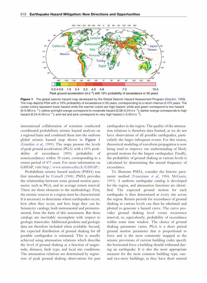
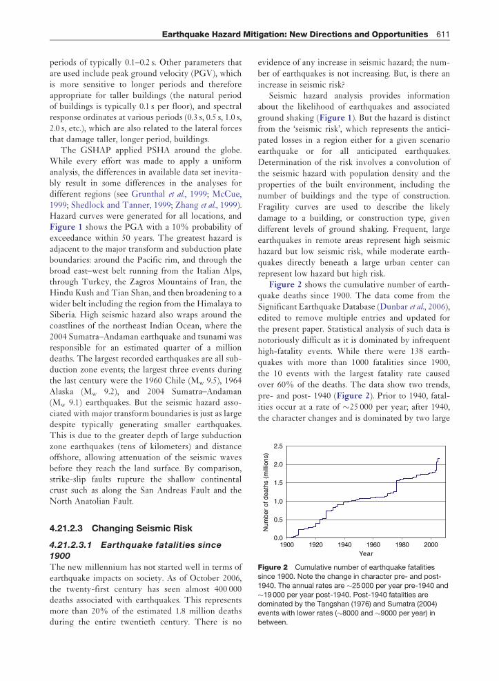
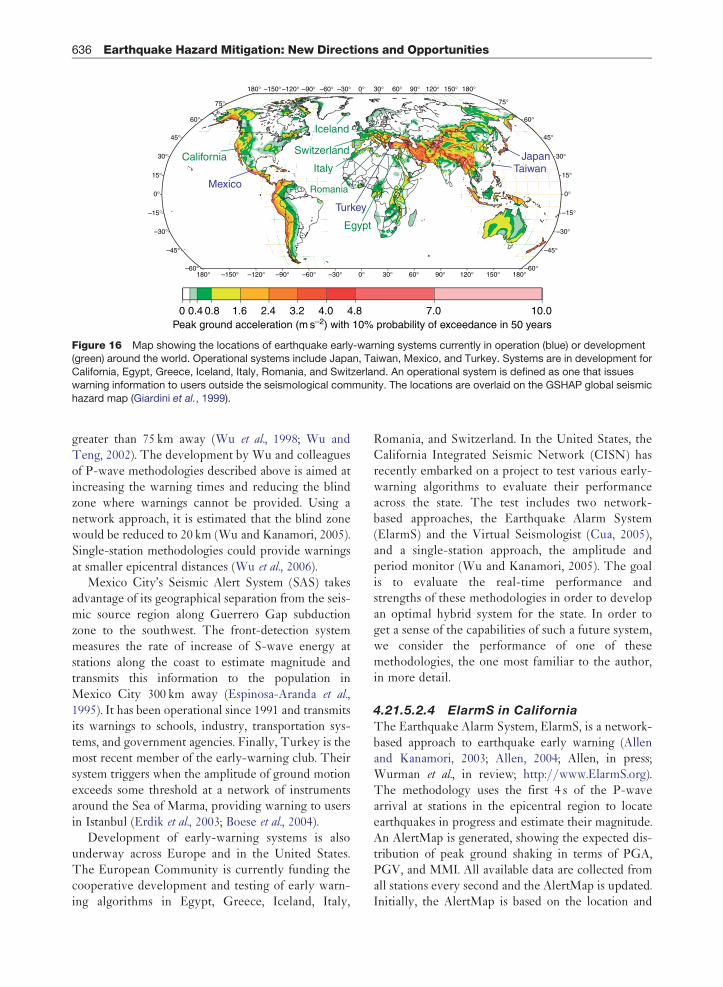
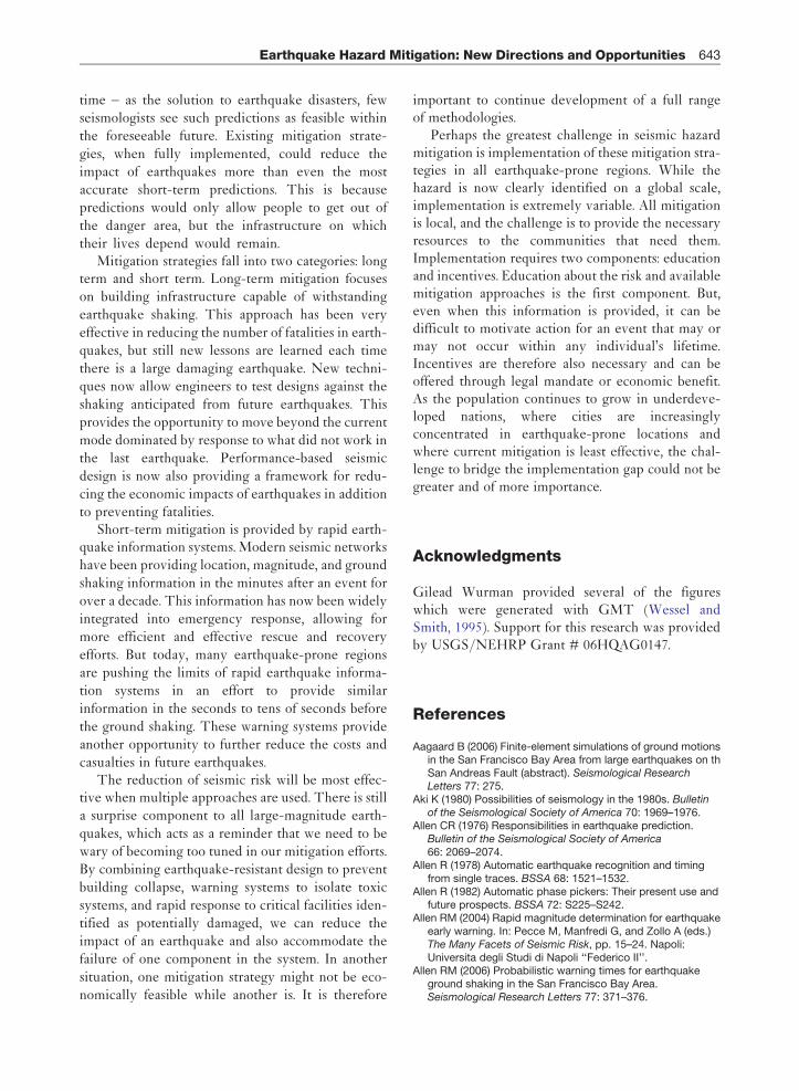
international collaboration of scientists conductedcoordinated probabilistic seismic hazard analyses ona regional basis and combined them into the uniformglobal seismic hazard map shown in Figure 1(Giardini et al., 1999). The maps present the levelsof peak ground acceleration (PGA) with a 10% prob-ability of exceedance (90% probability ofnonexceedance) within 50 years, corresponding to areturn period of 475 years. For more information onGSHAP, visit http://www.seismo.ethz.ch/GSHAP/.

Probabilistic seismic hazard analysis (PSHA) wasfirst introduced by Cornell (1968). PSHA providesthe relationship between some ground motion para-meter, such as PGA, and its average return interval.There are three elements to the methodology. First,the seismic sources in a region must be characterized.It is necessary to determine where earthquakes occur,how often they occur, and how large they can be.Seismicity catalogs, both instrumental and preinstru-mental, form the basis of this assessment. But thesecatalogs are inevitably incomplete with respect togeologic timescales. Additional geodetic and geologicdata are therefore included when available. Second,the expected distribution of ground shaking for allpossible earthquakes is estimated. This is usuallyachieved using attenuation relations which describethe level of ground shaking as a function of magni-tude, distance, fault type, and local site conditions.The attenuation relations are determined by regres-sion of peak ground shaking observations for past

earthquakes in the region. The quality of the attenua-tion relations is therefore data-limited, as we do nothave observations of all possible earthquakes, parti-cularly the larger infrequent events. For this reason,theoretical modeling of waveform propagation is nowbeing used to improve our understanding of likelyground motions for the largest earthquakes. Finally,the probability of ground shaking at various levels iscalculated by determining the annual frequency ofexceedance.

To illustrate PSHA, consider the historic para-meter method (Veneziano et al., 1984; McGuire,1993). A uniform earthquake catalog is developedfor the region, and attenuation functions are identi-fied. The expected ground motion for eachearthquake is then determined at every site acrossthe region. Return periods for exceedance of groundshaking at various levels can then be tabulated andplotted to generate a hazard curve. The curve pro-vides ground shaking level versus recurrenceinterval, or, equivalently, probability of exceedancewithin some time window. The choice of groundshaking parameter varies. PGA is a short periodground motion parameter that is proportional toforce and is the most commonly mapped as theseismic provisions of current building codes specifythe horizontal force a building should withstand dur-ing an earthquake. It is also the most appropriatemeasure for the most common building type, one-and two-story buildings, as they have short natural

Peak ground acceleration (m s–2) with 10% probability of exceedance in 50 years0 0.4

180°

75°

60°

45°

30°

15°

0°

–15°

–30°

–45°

–60°180° –150° –120° –90° –60° –30° 0° 30° 60° 90° 120° 150° 180°

–60°

–45°

–30°

–15°

0°

15°

30°

45°

60°

75°

–150°–120° –90° –60° –30° 0° 30° 60° 90° 120° 150° 180°

0.8 1.6 2.4 3.2 4.0 4.8 7.0 10.0

Romania

ItalyCalifornia

Iceland

Switzerland

Egypt

JapanTaiwan

Mexico

Turkey

Figure 1 The global seismic hazard map developed by the Global Seismic Hazard Assessment Program (Giardini, 1999).The map depicts PGA with a 10% probability of exceedance in 50 years, corresponding to a return interval of 475 years. Thecooler colors represent lower hazard while the warmer colors are high hazard: white and green correspond to low hazard(0–0.08ms!2 ); yellow and light orange correspond to moderate hazard (0.08–0.24ms!2); darker orange corresponds to highhazard (0.24–0.40ms!2 ); and red and pink correspond to very high hazard (> 0.40ms!2).


http://www.seismo.ethz.ch/GSHAP/

periods of typically 0.1–0.2 s. Other parameters thatare used include peak ground velocity (PGV), whichis more sensitive to longer periods and thereforeappropriate for taller buildings (the natural periodof buildings is typically 0.1 s per floor), and spectralresponse ordinates at various periods (0.3 s, 0.5 s, 1.0 s,2.0 s, etc.), which are also related to the lateral forcesthat damage taller, longer period, buildings.

The GSHAP applied PSHA around the globe.While every effort was made to apply a uniformanalysis, the differences in available data set inevita-bly result in some differences in the analyses fordifferent regions (see Grunthal et al., 1999; McCue,1999; Shedlock and Tanner, 1999; Zhang et al., 1999).Hazard curves were generated for all locations, andFigure 1 shows the PGA with a 10% probability ofexceedance within 50 years. The greatest hazard isadjacent to the major transform and subduction plateboundaries: around the Pacific rim, and through thebroad east–west belt running from the Italian Alps,through Turkey, the Zagros Mountains of Iran, theHindu Kush and Tian Shan, and then broadening to awider belt including the region from the Himalaya toSiberia. High seismic hazard also wraps around thecoastlines of the northeast Indian Ocean, where the2004 Sumatra–Andaman earthquake and tsunami wasresponsible for an estimated quarter of a milliondeaths. The largest recorded earthquakes are all sub-duction zone events; the largest three events duringthe last century were the 1960 Chile (Mw 9.5), 1964Alaska (Mw 9.2), and 2004 Sumatra–Andaman(Mw 9.1) earthquakes. But the seismic hazard asso-ciated with major transform boundaries is just as largedespite typically generating smaller earthquakes.This is due to the greater depth of large subductionzone earthquakes (tens of kilometers) and distanceoffshore, allowing attenuation of the seismic wavesbefore they reach the land surface. By comparison,strike-slip faults rupture the shallow continentalcrust such as along the San Andreas Fault and theNorth Anatolian Fault.

4.21.2.3 Changing Seismic Risk

4.21.2.3.1 Earthquake fatalities since1900The new millennium has not started well in terms ofearthquake impacts on society. As of October 2006,the twenty-first century has seen almost 400 000deaths associated with earthquakes. This representsmore than 20% of the estimated 1.8 million deathsduring the entire twentieth century. There is no

evidence of any increase in seismic hazard; the num-ber of earthquakes is not increasing. But, is there anincrease in seismic risk?

Seismic hazard analysis provides informationabout the likelihood of earthquakes and associatedground shaking (Figure 1). But the hazard is distinctfrom the ‘seismic risk’, which represents the antici-pated losses in a region either for a given scenarioearthquake or for all anticipated earthquakes.Determination of the risk involves a convolution ofthe seismic hazard with population density and theproperties of the built environment, including thenumber of buildings and the type of construction.Fragility curves are used to describe the likelydamage to a building, or construction type, givendifferent levels of ground shaking. Frequent, largeearthquakes in remote areas represent high seismichazard but low seismic risk, while moderate earth-quakes directly beneath a large urban center canrepresent low hazard but high risk.

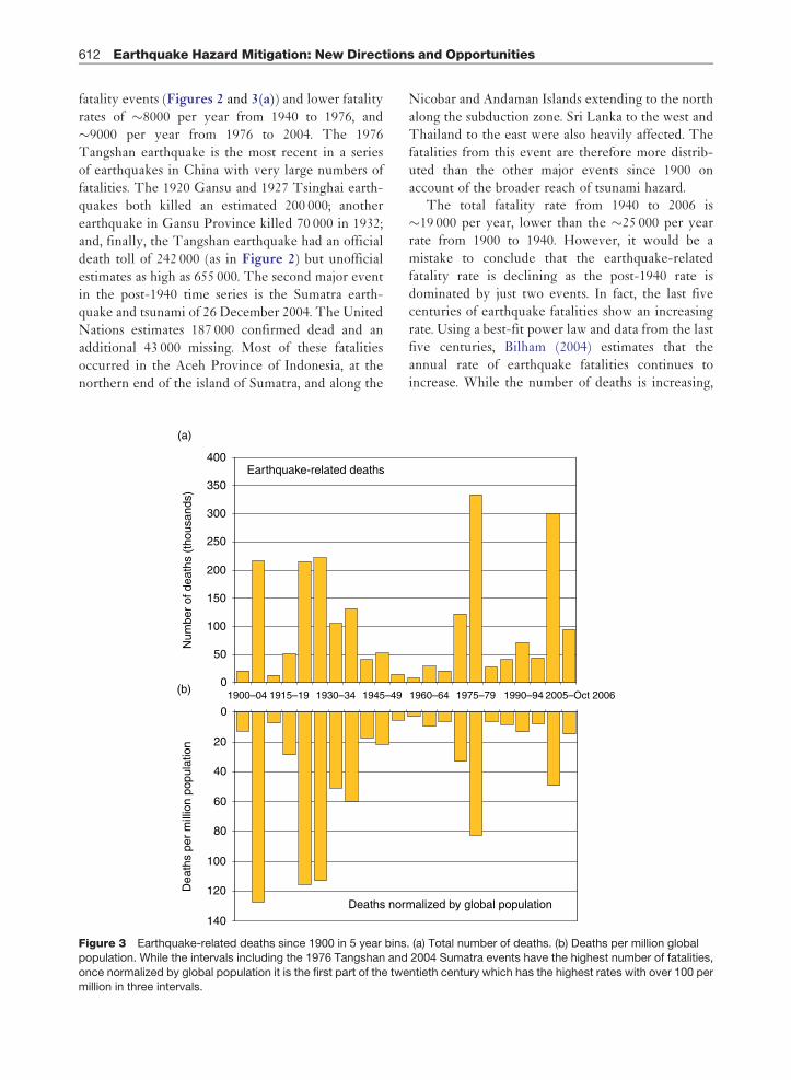
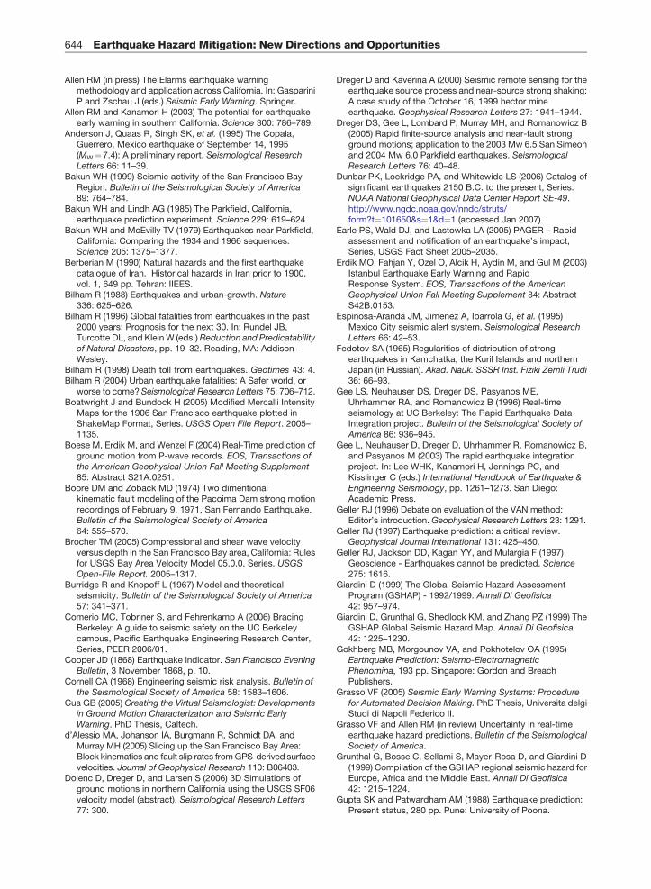
Figure 2 shows the cumulative number of earth-quake deaths since 1900. The data come from theSignificant Earthquake Database (Dunbar et al., 2006),edited to remove multiple entries and updated forthe present paper. Statistical analysis of such data isnotoriously difficult as it is dominated by infrequenthigh-fatality events. While there were 138 earth-quakes with more than 1000 fatalities since 1900,the 10 events with the largest fatality rate causedover 60% of the deaths. The data show two trends,pre- and post- 1940 (Figure 2). Prior to 1940, fatal-ities occur at a rate of "25 000 per year; after 1940,the character changes and is dominated by two large

1900 1920 1940 1960 1980 2000Year

2.5

2.0

1.5

1.0

0.5

0.0

Num

ber

of d

eath

s (m

illio

ns)

Figure 2 Cumulative number of earthquake fatalitiessince 1900. Note the change in character pre- and post-1940. The annual rates are "25000 per year pre-1940 and"19000 per year post-1940. Post-1940 fatalities aredominated by the Tangshan (1976) and Sumatra (2004)events with lower rates ("8000 and "9000 per year) inbetween.


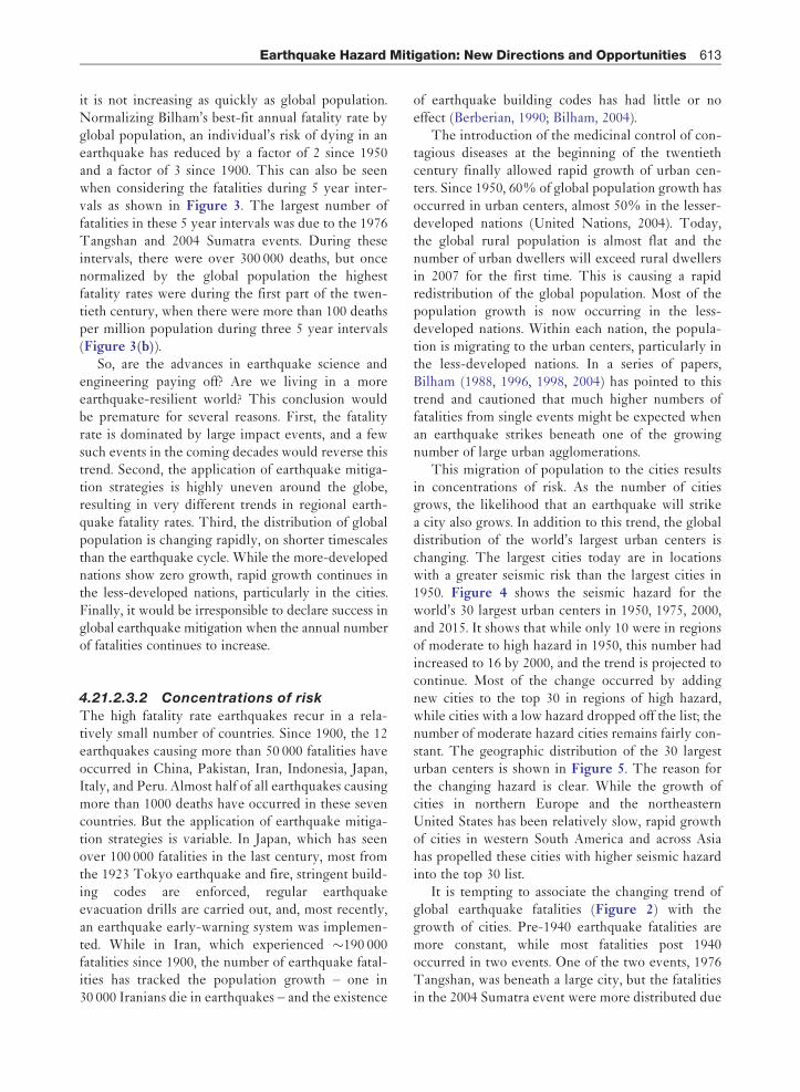
fatality events (Figures 2 and 3(a)) and lower fatalityrates of "8000 per year from 1940 to 1976, and"9000 per year from 1976 to 2004. The 1976Tangshan earthquake is the most recent in a seriesof earthquakes in China with very large numbers offatalities. The 1920 Gansu and 1927 Tsinghai earth-quakes both killed an estimated 200 000; anotherearthquake in Gansu Province killed 70 000 in 1932;and, finally, the Tangshan earthquake had an officialdeath toll of 242 000 (as in Figure 2) but unofficialestimates as high as 655 000. The second major eventin the post-1940 time series is the Sumatra earth-quake and tsunami of 26 December 2004. The UnitedNations estimates 187 000 confirmed dead and anadditional 43 000 missing. Most of these fatalitiesoccurred in the Aceh Province of Indonesia, at thenorthern end of the island of Sumatra, and along the

Nicobar and Andaman Islands extending to the northalong the subduction zone. Sri Lanka to the west andThailand to the east were also heavily affected. Thefatalities from this event are therefore more distrib-uted than the other major events since 1900 onaccount of the broader reach of tsunami hazard.

The total fatality rate from 1940 to 2006 is"19 000 per year, lower than the "25 000 per yearrate from 1900 to 1940. However, it would be amistake to conclude that the earthquake-relatedfatality rate is declining as the post-1940 rate isdominated by just two events. In fact, the last fivecenturies of earthquake fatalities show an increasingrate. Using a best-fit power law and data from the lastfive centuries, Bilham (2004) estimates that theannual rate of earthquake fatalities continues toincrease. While the number of deaths is increasing,

(a)

(b)

400

350

300

250

Num

ber

of d

eath

s (t

hous

ands

)D

eath

s pe

r m

illio

n po

pula

tion

200

150

100

50

0

01900–04 1915–19 1930–34 1945–49 1960–64 1975–79 1990–94 2005–Oct 2006

20

40

60

80

100

Deaths normalized by global population

Earthquake-related deaths

140

120

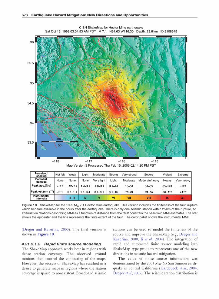
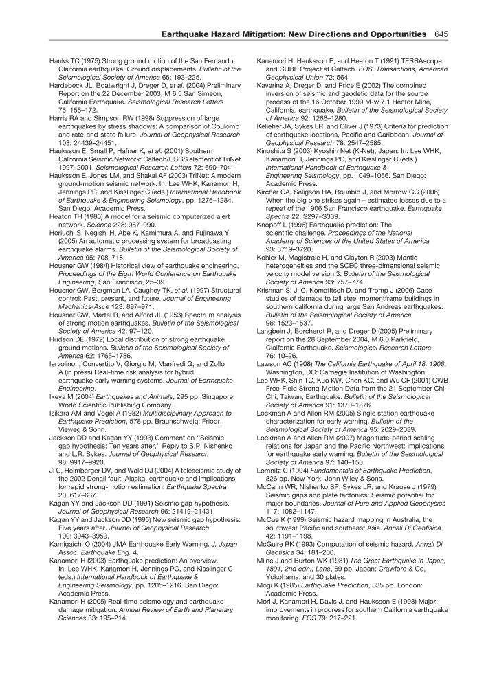
Figure 3 Earthquake-related deaths since 1900 in 5 year bins. (a) Total number of deaths. (b) Deaths per million globalpopulation. While the intervals including the 1976 Tangshan and 2004 Sumatra events have the highest number of fatalities,once normalized by global population it is the first part of the twentieth century which has the highest rates with over 100 permillion in three intervals.


it is not increasing as quickly as global population.Normalizing Bilham’s best-fit annual fatality rate byglobal population, an individual’s risk of dying in anearthquake has reduced by a factor of 2 since 1950and a factor of 3 since 1900. This can also be seenwhen considering the fatalities during 5 year inter-vals as shown in Figure 3. The largest number offatalities in these 5 year intervals was due to the 1976Tangshan and 2004 Sumatra events. During theseintervals, there were over 300 000 deaths, but oncenormalized by the global population the highestfatality rates were during the first part of the twen-tieth century, when there were more than 100 deathsper million population during three 5 year intervals(Figure 3(b)).

So, are the advances in earthquake science andengineering paying off? Are we living in a moreearthquake-resilient world? This conclusion wouldbe premature for several reasons. First, the fatalityrate is dominated by large impact events, and a fewsuch events in the coming decades would reverse thistrend. Second, the application of earthquake mitiga-tion strategies is highly uneven around the globe,resulting in very different trends in regional earth-quake fatality rates. Third, the distribution of globalpopulation is changing rapidly, on shorter timescalesthan the earthquake cycle. While the more-developednations show zero growth, rapid growth continues inthe less-developed nations, particularly in the cities.Finally, it would be irresponsible to declare success inglobal earthquake mitigation when the annual numberof fatalities continues to increase.

4.21.2.3.2 Concentrations of riskThe high fatality rate earthquakes recur in a rela-tively small number of countries. Since 1900, the 12earthquakes causing more than 50 000 fatalities haveoccurred in China, Pakistan, Iran, Indonesia, Japan,Italy, and Peru. Almost half of all earthquakes causingmore than 1000 deaths have occurred in these sevencountries. But the application of earthquake mitiga-tion strategies is variable. In Japan, which has seenover 100 000 fatalities in the last century, most fromthe 1923 Tokyo earthquake and fire, stringent build-ing codes are enforced, regular earthquakeevacuation drills are carried out, and, most recently,an earthquake early-warning system was implemen-ted. While in Iran, which experienced "190 000fatalities since 1900, the number of earthquake fatal-ities has tracked the population growth – one in30 000 Iranians die in earthquakes – and the existence

of earthquake building codes has had little or noeffect (Berberian, 1990; Bilham, 2004).

The introduction of the medicinal control of con-tagious diseases at the beginning of the twentiethcentury finally allowed rapid growth of urban cen-ters. Since 1950, 60% of global population growth hasoccurred in urban centers, almost 50% in the lesser-developed nations (United Nations, 2004). Today,the global rural population is almost flat and thenumber of urban dwellers will exceed rural dwellersin 2007 for the first time. This is causing a rapidredistribution of the global population. Most of thepopulation growth is now occurring in the less-developed nations. Within each nation, the popula-tion is migrating to the urban centers, particularly inthe less-developed nations. In a series of papers,Bilham (1988, 1996, 1998, 2004) has pointed to thistrend and cautioned that much higher numbers offatalities from single events might be expected whenan earthquake strikes beneath one of the growingnumber of large urban agglomerations.

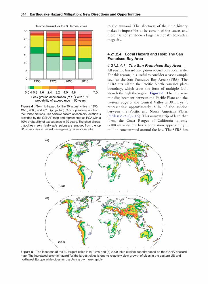
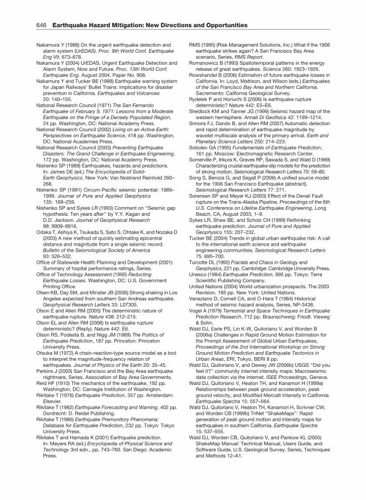
This migration of population to the cities resultsin concentrations of risk. As the number of citiesgrows, the likelihood that an earthquake will strikea city also grows. In addition to this trend, the globaldistribution of the world’s largest urban centers ischanging. The largest cities today are in locationswith a greater seismic risk than the largest cities in1950. Figure 4 shows the seismic hazard for theworld’s 30 largest urban centers in 1950, 1975, 2000,and 2015. It shows that while only 10 were in regionsof moderate to high hazard in 1950, this number hadincreased to 16 by 2000, and the trend is projected tocontinue. Most of the change occurred by addingnew cities to the top 30 in regions of high hazard,while cities with a low hazard dropped off the list; thenumber of moderate hazard cities remains fairly con-stant. The geographic distribution of the 30 largesturban centers is shown in Figure 5. The reason forthe changing hazard is clear. While the growth ofcities in northern Europe and the northeasternUnited States has been relatively slow, rapid growthof cities in western South America and across Asiahas propelled these cities with higher seismic hazardinto the top 30 list.

It is tempting to associate the changing trend ofglobal earthquake fatalities (Figure 2) with thegrowth of cities. Pre-1940 earthquake fatalities aremore constant, while most fatalities post 1940occurred in two events. One of the two events, 1976Tangshan, was beneath a large city, but the fatalitiesin the 2004 Sumatra event were more distributed due


to the tsunami. The shortness of the time historymakes it impossible to be certain of the cause, andthere has not yet been a large earthquake beneath amegacity.

4.21.2.4 Local Hazard and Risk: The SanFrancisco Bay Area

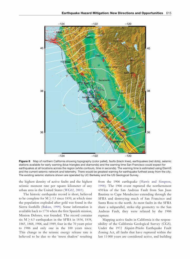
4.21.2.4.1 The San Francisco Bay AreaAll seismic hazard mitigation occurs on a local scale.For this reason, it is useful to consider a case examplesuch as the San Francisco Bay Area (SFBA). TheSFBA sits within the Pacific–North America plateboundary, which takes the form of multiple faultstrands through the region (Figure 6). The interseis-mic displacement between the Pacific Plate and thewestern edge of the Central Valley is 38mmyr!1,representing approximately 80% of the motionbetween the Pacific and North American Plates(d’Alessio et al., 2005). This narrow strip of land thatforms the Coast Ranges of California is only"100 km wide but has a population approaching 7million concentrated around the bay. The SFBA has

Seismic hazard for the 30 largest cities

30

25

20

15

10

5

01950

0 0.4 0.8 1.6 2.4 3.2 4.0 4.8 7.0Peak ground acceleration (m s–2) with 10%

probability of exceedance in 50 years

1975 2000 2015

Figure 4 Seismic hazard for the 30 largest cities in 1950,1975, 2000, and 2015 (projected). City population data fromthe United Nations. The seismic hazard at each city location isprovided by the GSHAP map and represented as PGA with a10% probability of exceedance in 50 years. The chart showsthat cities in seismically safe regions are removed from the top30 list as cities in hazardous regions grow more rapidly.

(a)

(b)

1950

2000

Figure 5 The locations of the 30 largest cities in (a) 1950 and (b) 2000 (blue circles) superimposed on the GSHAP hazardmap. The increased seismic hazard for the largest cities is due to relatively slow growth of cities in the eastern US andnorthwest Europe while cities across Asia grow more rapidly.


the highest density of active faults and the highestseismic moment rate per square kilometer of anyurban area in the United States (WG02, 2003).

The historic earthquake record is short, believedto be complete for M# 5.5 since 1850, at which timethe population exploded after gold was found in theSierra foothills (Bakun, 1999). Some information isavailable back to 1776 when the first Spanish mission,Mission Delores, was founded. The record containssix M# 6.5 earthquakes in the SFBA in 1836, 1838,1865, 1868, 1906, and 1989, four in the 70 years priorto 1906 and only one in the 100 years since.This change in the seismic energy release rate isbelieved to be due to the ‘stress shadow’ resulting

from the 1906 earthquake (Harris and Simpson,1998). The 1906 event ruptured the northernmost450 km of the San Andreas Fault from San JuanBautista to Cape Mendocino extending through theSFBA and destroying much of San Francisco andSanta Rosa to the north. As most faults in the SFBAshare a subparallel, strike-slip geometry to the SanAndreas Fault, they were relaxed by the 1906rupture.

Mapping active faults in California is the respon-sibility of the California Geological Survey (CGS).Under the 1972 Alquist-Priolo Earthquake FaultZoning Act, all faults that have ruptured within thelast 11 000 years are considered active, and building

–124 –122 –120

40

38

36

–120–122–124

36

38

40

Fort Bragg

Redding

Susanville

Chico

Grass valley

Reno

South Lake

Eureka

70

60

Ukiah

Sacramento

San Francisco

Santa Rosa

Modesto

Sonora

Merced

Fresho

Baker

3040

60

50 Visalia

Monterey

Coalinga

San Jose

20

10

0

10

20

PasoRobles

Hollister

King city

Figure 6 Map of northern California showing topography (color pallet), faults (black lines), earthquakes (red dots), seismicstations available for early warning (blue triangles and diamonds) and the warning time San Francisco could expect forearthquakes at all locations across the region (white contours, time in seconds). The warning time is estimated using ElarmSand the current seismic network and telemetry. There would be greatest warning for earthquake furthest away from the city.The existing seismic stations shown are operated by UC Berkeley and the US Geological Survey.


close to these known faults is tightly regulated toensure that buildings are at least 50 feet from thefault trace. The CGS is now also in the process ofmapping other seismic hazards including liquefactionand landslide hazards during earthquakes.

The Southern California Earthquake Center(SCEC) is a collaboration of earthquake scientistsworking with the goal of understanding the earth-quake process and mitigating the associated hazards.While SCEC is focused on the earthquake problemin southern California, the methodologies developedby SCEC scientists to quantify earthquake probabil-ities and the shaking hazards associated with them areapplicable everywhere, including in our chosenregion of focus, the SFBA.

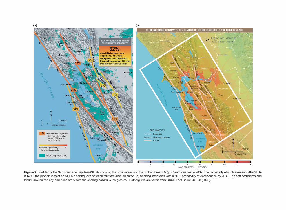
4.21.2.4.2 Earthquake probabilitiesTo evaluate the probability of future earthquakes andground shaking in the region, the US GeologicalSurvey established a Working Group on EarthquakeProbabilities. In several incarnations starting in 1988,the group has collected data and applied the most up-to-date methodologies available to estimate long-term earthquake probabilities drawing on input froma broad cross section of the Earth science community.The most recent study (hereafter WG02) was com-pleted in 2002 (WG02, 2003). In it, the probabilities ofone or more earthquakes in the SFBA, on one of theseven identified fault systems, between 2002 and 2032were estimated. The likely intensities of ground shak-ing were also combined to produce a probabilisticseismic hazard map for the region, similar to theGSHAP map discussed above. The WG02 resultsare shown in Figure 7.

The earthquake model used to estimate theseprobabilities has three elements. The first is a time-independent forecast of the average magnitudes andrates of occurrence of earthquakes on the majoridentified fault segments. It is derived from thepast earthquake catalog. The second elementincludes four time-dependent models of theearthquake process to include the effects of theearthquake cycle and interactions between the faultsystems. The concept of the earthquake cycle holdsthat after a major earthquake and associatedaftershocks, another major rupture is not possibleuntil the elastic strain has reaccumulated (Reid’selastic rebound theory). As time goes by, theprobability of an earthquake therefore increases. Amajor earthquake also reduces the stress on any adja-cent faults with a similar orientation, generating astress shadow. This has been observed both in

numerical models and in the reduced seismicity onfaults adjacent to the San Andreas after the 1906rupture. In the SFBA, both the 1906 event and themore recent 1989 earthquake cast stress shadows.The third element of the earthquake model charac-terizes the rates of background seismicity, that is,earthquakes that do not occur on the seven majorfault systems. The 1989 Loma Prieta event was onesuch earthquake. These various earthquake modelsprovide different estimates of earthquake probabil-ities. WG02 uses expert opinion to determine therelative weight for each probability estimate derivedfrom each model.

Figure 7 shows the WG02 results. It is estimatedthat there is a 62% probability of one or more M# 6.7earthquakes in the SFBA from 2002 to 2032. As shownin Figure 7(a), the probability of one or more M# 6.7events is greatest on the Hayward–Rodgers Creekand San Andreas Faults, which have probabilities of27% and 21%, respectively. The estimated uncer-tainties in these numbers are substantial. For theSFBA the 95% confidence bounds are 37% to 87%.For the Hayward–Rodgers Creek and San AndreasFaults, the bounds are 10–58% and 2–45%, respec-tively. A critical source of this uncertainty is theextent to which the SFBA has emerged fromthe stress shadow of the 1906 earthquake. Simpleelastic interaction models suggest that the regionshould have emerged from the stress shadow, whilethe low seismicity rates for the last century wouldsuggest that the SFBA remains within the shadow.Rheological models of the crust and uppermostmantle, and perhaps the 1989 Loma Prieta earth-quake, suggest that the region may just be emergingnow. If the region is emerging, then it can expect anincrease in the number of major events over the nextfew decades.

4.21.2.4.3 Future lossesJust as the world has not experienced a major earth-quake beneath a megacity, the US has notexperienced a major earthquake directly beneathone of its cities. The two most damaging earthquakeswere the 1989 Loma Prieta earthquake (which wasbeneath the rugged mountains 100 km south of SanFrancisco and Oakland) and the 1994 Northridgeearthquake (which, although centered beneath thepopulated San Fernando Valley, caused strongestground shaking in the sparsely populated SantaSuzanna Mountains to the north). Each event caused"60 deaths and the estimated damages were $10 and


(a) (b)

Figure 7 (a) Map of the San Francisco Bay Area (SFBA) showing the urban areas and the probabilities of M#6.7 earthquakes by 2032. The probability of such an event in the SFBAis 62%, the probabilities of an M# 6.7 earthquake on each fault are also indicated. (b) Shaking intensities with a 50% probability of exceedance by 2032. The soft sediments andlandfill around the bay and delta are where the shaking hazard is the greatest. Both figures are taken from USGS Fact Sheet 039-03 (2003).

$46 billion for Loma Prieta and Northridge, respec-tively (in 2000-dollars). While the impacts weresignificant, the events were relatively moderate indamage.

The ground shaking estimates, such as those thatare part of WG02, provide the basis for loss estima-tion. Loss estimation methodologies use data on thelocations and types of buildings, ground shakingmaps for scenario or past earthquakes, and fragilitycurves relating the extent of damage to the groundshakng for each building type, to estimate the totaldamage from the event. The worst-case scenarioconsidered for northern California is a repeat of the1906 earthquake. The losses have been estimated at$170–225 billion for all related losses including sec-ondary fires and toxic releases (RMS, 1995), a factorof 2 greater than the $90–120 billion loss estimate forproperty alone (Kircher et al., 2006). It is estimatedthat the number of deaths could range from 800 to3400 depending on the time of day, and 160 000–250 000 households will be displaced (Kircher et al.,2006). An earthquake rupturing the length of theHayward–Rodgers Creek Fault is estimated tocause $40 billion in damage to buildings alone(Rowshandel, 2006).

These estimates of seismic hazard and risk pro-vide a quantitative basis for earthquake hazardmitigation in the region. The choice of a relativelyshort, 30-year time window by WG02 has the advan-tage that it is a similar timescale to that of propertyownership. But, as pointed out above and by WG02,the reliability of PSHA analysis decreases as thetemporal and spatial scales decrease. Our observa-tions of large (M> 6.5) earthquakes in California arelimited. Many of the recent damaging eartthquakesoccurred on faults that had not been recognized,including the two most damaging earthquakes, the1989 Loma Prieta and 1994 Northridge events. While‘background seismicity’ is included in the seismichazard estimates, these events are a reminder of thelimitations to our current understanding of theearthquake hazard. These hazard and risk estimatesare therefore most appropriately used to motivatebroad efforts to mitigate seismic hazard acrossthe entire SFBA rather than efforts along aspecific fault segment. The limitations in our obser-vational data set also caution against becoming too‘tuned’ in mitigation strategy. The use of multiplemitigation strategies will prevent over-reliance on asingle, and possibly limited, model of future earth-quake effects.

4.21.3 The ‘Holy Grail’ of Seismology:Earthquake Prediction

‘‘When is the big one?’’ is the first question asked byevery member of the public or press when they visitthe Berkeley Seismological Laboratory. Answeringthis question, predicting an earthquake, is oftenreferred to as the Holy Grail of seismology. In thiscontext, a prediction means anticipating the time,place, and magnitude of a large earthquake within anarrow window and with a high enough probabilitythat preparations for its effects can be undertaken(Allen, 1976). For the general public, answering thisquestion is the primary responsibility of the seismo-logical community.

The public considers earthquake predictionimportant because it would allow evacuation of citiesand prevention of injury and loss of life in damagedand collapsed buildings. However, the seismologyand engineering communities have already devel-oped a strategy to prevent building collapse byidentifying the likely levels of ground shaking anddesigning earthquake-resistant buildings that areunlikely to collapse. Once building codes for earth-quake-resistant buildings are fully implemented,earthquake prediction would not be as important.But even before full implementation of buildingcodes, earthquake prediction would only be partiallysuccessful as it would be capable of mitigatingimmediate and not long-term impacts of earthquakes.A prediction would allow for evacuations, but theensuing earthquake would leave the urban area unin-habitable and only a fraction of the prior occupantswould likely return.

It is possible to make high-probability short-termpredictions for hurricanes as was done in the case ofHurricane Katrina in August 2005. Still, an estimated1800 people were killed when New Orleans andother areas of Louisiana and Mississippi were inun-dated by flood waters. In New Orleans, 80% of thecity was flooded, destroying much of the housing andinfrastructure, and it is not yet clear what proportionwill be replaced. One year later, the population ofNew Orleans was less than half its pre-Katrina leveland roughly equivalent to what it was in 1880. If thebuilt environment was designed to withstand a hur-ricane of Katrina’s strength, these lives would nothave been lost and New Orleans would still bethriving.

For the scientific community, earthquake predic-tion has a much broader meaning, encompassing


the physics of the earthquake process at all time-scales. The long-term probabilistic forecastsdescribed in the previous section are predictions,but they have low probabilities of occurrence overlarge time windows. There is currently no approachthat has consistently predicted large-magnitudeearthquakes and most seismologists do not expectsuch short-term predictions in the foreseeable future.While many advances have been made in under-standing crustal deformation, stress accumulation,rupture dynamics, friction and constitutive relations,fault interactions, and linear dynamics, a lack ofunderstanding of the underlying physics and diffi-culty in making detailed field observations mappingthe spatial and temporal variations in structure,strain, and fault properties makes accurate short-term predictions difficult.

In addition to these observational constraints,earthquakes are part of a complex process in whichdistinct structures such as faults interact with thediffuse heterogeneity of the Earth’s crust and mantleat all scales. Even simple mechanical models of theearthquake process show chaotic behavior (Burridgeand Knopoff, 1967; Otsuka, 1972; Turcotte, 1992),suggesting it will be difficult to predict earthquakesin a deterministic way. Instead, it may only be possi-ble to make predictions in a statistical sense withconsiderable uncertainty (Turcotte, 1992).Kanamori (2003) details the important sources ofuncertainty: (1) the stress accumulation due to rela-tively constant plate motion can be modified locallyby proximal earthquakes; (2) the strength of the seis-mogenic zone may change with time, say due to themigration of fluids; (3) predicting the size of an earth-quake may be difficult depending on whether a smallearthquake triggers a large one; (4) external forcesmay trigger events as observed in geothermal areasafter large earthquakes.

Despite these challenges, the search for the silverbullet – an earthquake precursor – continues. Aspointed out by Kanamori (2003), there are two typesof precursors. For the purpose of short-term earth-quake prediction, identification of a single precursorbefore all large magnitude events is desirable. To date,no such precursor has been identified as far as weknow. However, unusual precursory signals havebeen observed before one, or perhaps a few earth-quakes. These precursors may be observed beforefuture earthquakes and are therefore worthy ofresearch effort. The list of observed precursors includesincreased seismicity and strain, changes in seismicvelocities, electrical resistivity and potential, radio

frequency emission, and changes in ground waterlevels and chemistry (see Rikitake, 1986).

The one successful prediction of a major earth-quake was prior to the 1975 MS 7.3 Haicheng (China)event. More than 1 million people lived near theepicenter, and a recent evaluation of declassifieddocuments concludes that an evacuation ordered bya local county government saved thousands of lives(Wang et al., 2006). There were two official middle-term predictions (1–2 years). On the day of the earth-quake, various actions taken by provincial scientistsand government officials constituted an imminentprediction, although there was no official short-term(a few months) prediction. A foreshock sequenceconsisting of several hundred events triggered theimminent prediction; other precursors including geo-detic deformation, changes in groundwater level,chemistry, and color, and peculiar animal behaviorare also reported to have played a role (Wang et al.,2006). What is not known is how many false predic-tions were made prior to the evacuation, nor is itknown how many earthquake evacuation ordershave been made across China. The initial euphoriaover the successful evacuation was soon dampenedby the Tangshan earthquake the following year forwhich there was no prediction.

Extensive literature exists detailing the specifics ofthe various proposed earthquake prediction meth-odologies and other reported cases of earthquakeprediction (Rikitake, 1976; Vogel, 1979; Wyss, 1979;Isikara and Vogel, 1982; Rikitake, 1982; Unesco, 1984;Mogi, 1985; Rikitake, 1986; Gupta and Patwardham,1988; Olson et al., 1989; Wyss, 1991; Lomnitz, 1994;Gokhberg et al., 1995; Sobolev, 1995; Geller, 1996;Knopoff, 1996; Geller, 1997; Geller et al., 1997;Sykes et al., 1999; Rikitake and Hamada, 2001;Kanamori, 2003; Ikeya, 2004). Expert panels areused in many countries to evaluate earthquake pre-dictions and provide advice to governments and thepublic. In the US, the National Earthquake PredictionEvaluation Council (NEPEC) provides advice to thedirector of the US Geological Survey, and theCalifornia Earthquake Prediction Council (CEPEC)advises the Governor. No short-term earthquake pre-dictions have been made by these councils to date.

4.21.4 Long-Term Mitigation:Earthquake-Resistant Buildings

The implementation of building codes mandating theuse of earthquake-resistant buildings has been highly


successful in mitigating the impact of earthquakes insome regions. The number of fatalities has beenreduced, and the majority of direct economic lossesin recent US earthquakes (e.g., 1989 Loma Prieta,1994 Northridge, and 2001 Nisqually) were fromdamage to buildings and lifelines constructed before1976 when the Uniform Building Code was updatedfollowing the 1971 San Fernando earthquake(National Research Council, 2003). In the past, theimprovement of building design was undertaken inresponse to observations from previous earthquakes.While improvements are still largely in response topast earthquakes today, new seismological and engi-neering techniques allow the development of designcriteria for future likely earthquakes. Building designis also going beyond the prevention of collapse withthe goal of reducing the costs of future earthquakes inaddition to the number of fatalities. One of the chal-lenges is implementation of earthquake-resistantdesigns, both for new construction and for the exist-ing building stock.

4.21.4.1 Earthquake-Resistant Design

4.21.4.1.1 Lateral forcesFollowing the 1891 Nobi, Japan, earthquake thatkilled 7000 people, John Milne laid the foundationfor the building codes that were to follow (Milne andBurton, 1891). He detailed the poor performance ofmodern masonry construction which had recentlybeen introduced to replace the more traditionalwood construction in an effort to mitigate fires, anddescribed the great variability in damage to buildingsover short distances due to the effect of soft versushard ground. He also emphasized the need to designbuildings to withstand the horizontal forces asso-ciated with earthquakes rather than just verticalforces. Similar observations were made followingthe 1906 San Francisco earthquake by the LawsonCommission (1908).

After the 1908 Messina-Reggio earthquake insouthern Italy, which killed 83 000, Panetti proposedthat buildings be designed to withstand a horizontalforce in proportion to their vertical load. He sug-gested that the first story should be able towithstand 1/12th the weight of the overlying storiesand the second and third stories should be able towithstand 1/8th (Housner, 1984). In Japan, ToshikataSano made a similar proposal. In 1915, he recom-mended that buildings should be able to withstand alateral force, V, in proportion to their weight,W, suchthat V$CW, where C is the lateral force coefficient

expressed as a percentage of gravitational accelera-tion. But it was not until the 1923 Kanto earthquakewhich killed 100 000 that Sano’s criteria became partof the Japanese Urban Building Law EnforcementRegulations released in 1924 (Whittaker et al., 1998).In the Japanese regulations, C, was set at 10% g.Following the 1925 Santa Barbara earthquake in theUS, several communities adopted Sano’s criteria withC$ 20%g. Sano’s recommendation was also adoptedin the first release of the US Uniform Building Codein 1927, where the value of C was dependent on thesoil conditions (National Research Council, 2002).

4.21.4.1.2 Strong-motion observationsWhile building codes were mandating earthquake-resistant designs as early as the 1920s, there were stillno instrumental observations of the actual groundmotions responsible for building damage. Milne andcolleagues designed and built the first effective seis-mographs in Japan in the late 1880s. The firstinstruments in the US were installed at the LickObservatory of UC Berkeley in 1887 (Lawson,1908). By the 1920s, seismological observatories hadbeen established around the world, but they weredesigned to measure the weak (low-amplitude)motion resulting from distant earthquakes. It wasnot until the 1930s that broadband strong (high-amplitude) motion instruments were available, cap-able of recording both the low- and high-frequencyshaking responsible for the damage to buildings. The1933 Long Beach earthquake provided the firstinstrumental recording in which PGAs of 29%g inthe vertical and 20%g in the horizontal wereobserved. A larger PGA value of 33%g was observedat EI Centro a few years later on an instrument 10 kmfrom the 1940 M 7.1 Imperial Valley earthquakerupture. This remained the largest measured groundmotion for 25 years, establishing the EI Centro seis-mogram as the standard for earthquake engineeringin both the US and Japan.

Over the following decades, the strong-motiondatabase grew, but slowly. This changed in 1971when the M 6.6 San Fernando earthquake struckthe Los Angeles region and the number of strong-motion recordings more than doubled. In this earth-quake, more than 400 000 people experienced PGAin excess of 20%g, and it became clear that high-frequency PGA varied over short distances while thelonger period (10 s) displacements did not (NationalResearch Council, 1971; Hudson, 1972, Hanks, 1975).One instrument located on the abutment of thePacoima Dam recorded a 1m s!1 velocity pulse


shortly followed by a 120%g acceleration pulse(Boore and Zoback, 1974). The strong-motion data-base generated by this earthquake played animportant role in the updates to the UniversalBuilding Code, which followed in 1976. It is a testa-ment to the importance of strong-motion networks,and the earthquake engineering research they pro-vide for, that the majority of damage in recent USearthquakes (1989 Loma Prieta, 1994 Northridge,and 2001 Nisqually) occurred to structures builtprior to the 1976 update to the Uniform BuildingCode (National Research Council, 2003).

Strong-motion networks continue to provideimportant waveform data sets for damaging earth-quakes. One notable recent example was the 1999Mw 7.6 Chi-Chi earthquake, which occurred beneathcentral Taiwan on 20 September 1999. The strong-motion seismic network that had recently beendeployed by the Central Weather Bureau across theisland provided waveforms at 441 sites, includingover 60 recordings within 20 km of the fault ruptures(Lee et al., 2001). In addition to Taiwan, dense strong-motion networks with hundreds of instruments arenow operational in Japan and the western US. Manymore smaller networks are operational in earthquakeprone regions around the world. They all providecrucial data when a large earthquake occurs close by,yet the infrequency of such events makes continuousfunding and operation a challenge.

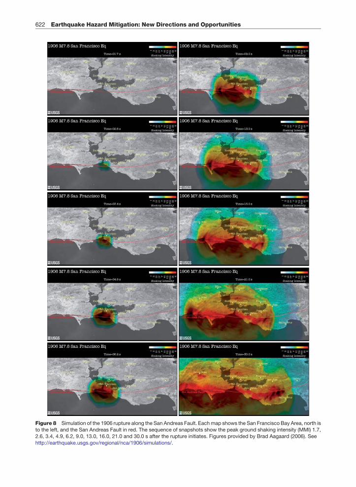
4.21.4.1.3 Strong-motion simulationsAdvances in computational capabilities, numericaltechniques, and our knowledge of the structure offault zone regions now make it feasible to simulateearthquakes to provide estimates of likely groundmotions in future events. The recent centennial ofthe 1906 San Francisco earthquake motivated onesuch study in northern California. In order to simu-late ground shaking, a velocity model was firstdeveloped for northern California. The geology-based model provides three-dimensional (3-D) velo-city and attenuation for the simulation usingobserved relationships between rock type, depth,and seismic parameters (Brocher, 2005). Seismic andgeodetic data available from the 1906 earthquakewere used to map the distribution of slip in spaceand time on the fault plane (Song et al., 2006). Severalnumerical techniques were then used to simulate theearthquake rupture through the geologic model. Thesimulations could be calibrated by comparing thecalculated peak intensities with observed intensitiesfrom the 1906 earthquake which were compiled into

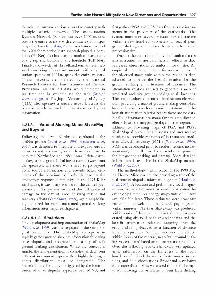
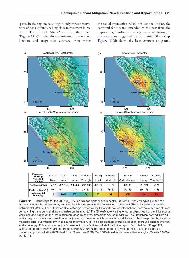
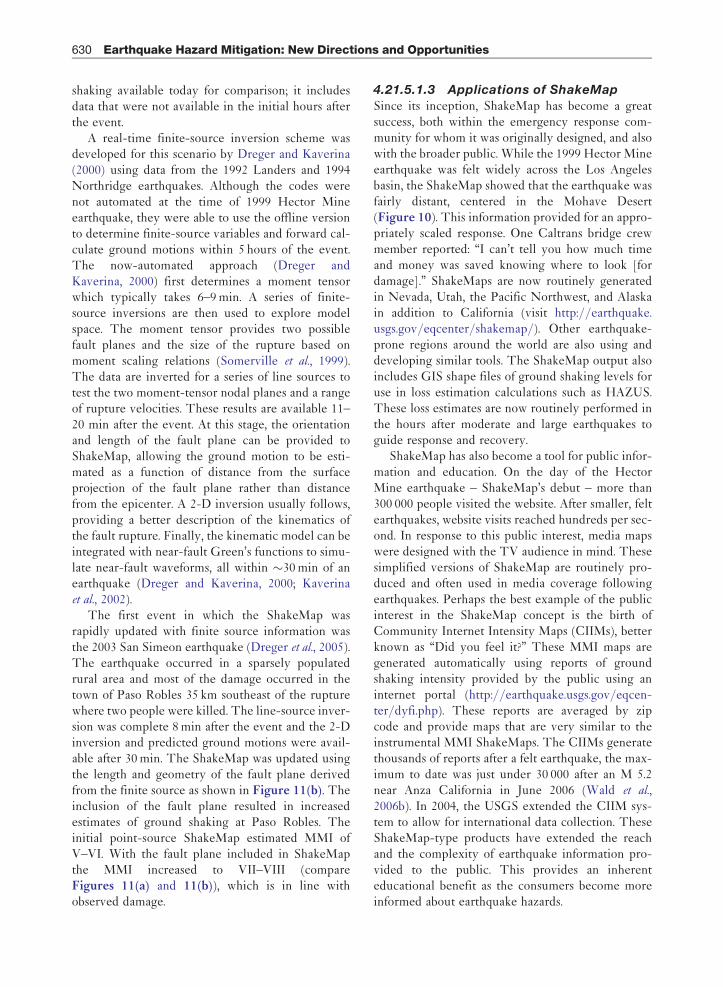
a 1906 ShakeMap (Lawson, 1908; Boatwright andBundock, 2005). Snap-shots from one of the simula-tions are shown in Figure 8, (Aagaard, 2006). Thepeak intensities generated by the simulations repro-duce the prominent features of the 1906 ShakeMapvalidating the simulations.

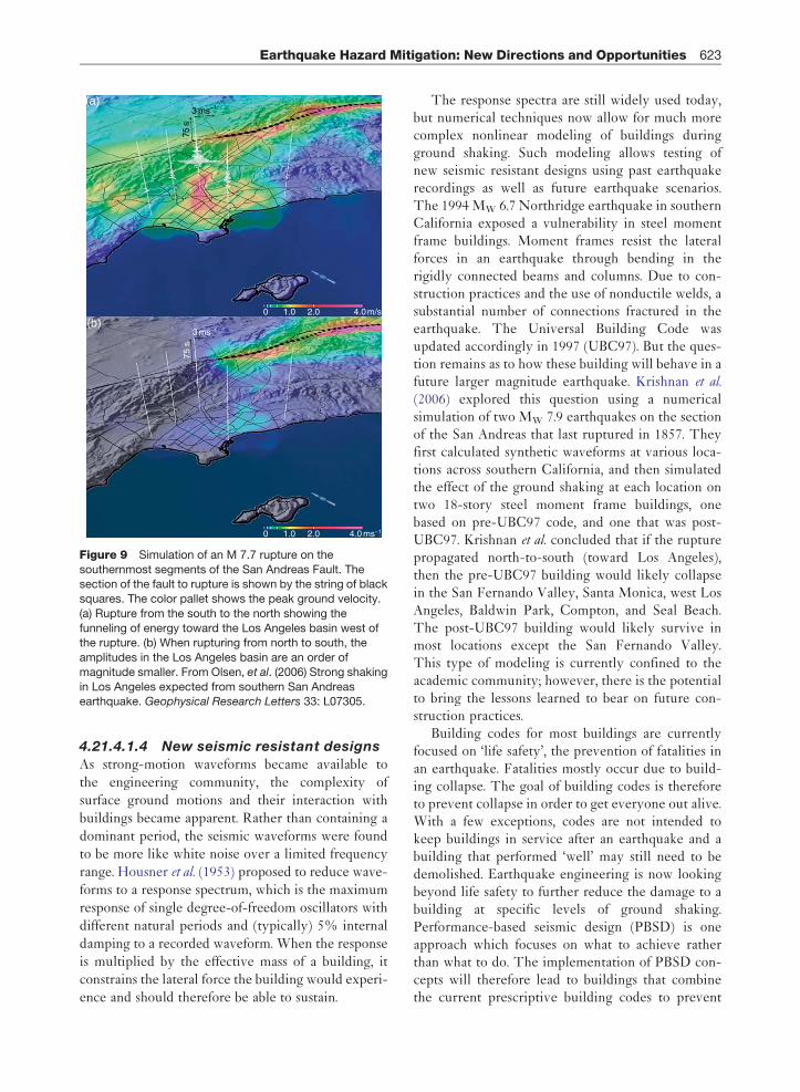
Other simulations of the 1989 Loma Prieta earth-quake, for which instrumental recording of groundshaking is available, also demonstrate that the simu-lations replicate the amplitude and duration of theobserved shaking at frequencies less than 0.5Hz(Aagaard, 2006; Dolenc et al., 2006). Given likelyslip distributions of future earthquakes, these simula-tions can now provide estimates of the groundshaking in the form of complete seismic waveforms.The results of one study on the southern San AndreasFault are shown in Figure 9 (Olsen et al., 2006). Thesource rupture is along the San BernardinoMountains and Coachella Valley segments, whichare considered more likely to rupture in the comingdecades as they have not ruptured since 1812 and1960. The slip distribution of the 2002 MW 7.9Denali, Alaska, earthquake was used for the ruptureafter scaling it for an M 7.7 rupture. The velocitystructure was provided by the SCEC CommunityVelocity Model (Kohler et al., 2003), and groundshaking is calculated for frequencies of 0–0.5Hz justas in the northern California simulations. When therupture propagates from the southeast to the north-west, the directivity effect produces large amplitudeground motions in the Los Angeles metropolitanregion. When the fault rupture is to the east of LosAngeles, the chain of sedimentary basins (the SanBernardino, Chino, San Gabriel, and Los Angelesbasins) running westward from the northern termina-tion of the rupture funnels seismic energy toward thedowntown. The seismograms superimposed onFigure 9 show velocities of more than 3m s!1.When the rupture propagates to the southeast, theground shaking in LA is an order of magnitude smal-ler (Olsen et al., 2006).

These simulations are providing new insights intoseismic wave propagation and help identify the geo-logic structures that control strong ground shaking.The uncertainties in the predicted ground shakingresult from limitations in the velocity models, thenumerical techniques, and the unknown future slipdistributions. However, these simulations allow us toexplore the range of possible ground motions that wemight expect for earthquake ruptures that are evidentin the geologic record but not the historic or instru-mental records.


Figure 8 Simulation of the 1906 rupture along the San Andreas Fault. Eachmap shows the San Francisco Bay Area, north isto the left, and the San Andreas Fault in red. The sequence of snapshots show the peak ground shaking intensity (MMI) 1.7,2.6, 3.4, 4.9, 6.2, 9.0, 13.0, 16.0, 21.0 and 30.0 s after the rupture initiates. Figures provided by Brad Aagaard (2006). Seehttp://earthquake.usgs.gov/regional/nca/1906/simulations/.


http://earthquake.usgs.gov/regional/nca/1906/simulations/

4.21.4.1.4 New seismic resistant designsAs strong-motion waveforms became available tothe engineering community, the complexity ofsurface ground motions and their interaction withbuildings became apparent. Rather than containing adominant period, the seismic waveforms were foundto be more like white noise over a limited frequencyrange. Housner et al. (1953) proposed to reduce wave-forms to a response spectrum, which is the maximumresponse of single degree-of-freedom oscillators withdifferent natural periods and (typically) 5% internaldamping to a recorded waveform. When the responseis multiplied by the effective mass of a building, itconstrains the lateral force the building would experi-ence and should therefore be able to sustain.

The response spectra are still widely used today,but numerical techniques now allow for much morecomplex nonlinear modeling of buildings duringground shaking. Such modeling allows testing ofnew seismic resistant designs using past earthquakerecordings as well as future earthquake scenarios.The 1994 MW 6.7 Northridge earthquake in southernCalifornia exposed a vulnerability in steel momentframe buildings. Moment frames resist the lateralforces in an earthquake through bending in therigidly connected beams and columns. Due to con-struction practices and the use of nonductile welds, asubstantial number of connections fractured in theearthquake. The Universal Building Code wasupdated accordingly in 1997 (UBC97). But the ques-tion remains as to how these building will behave in afuture larger magnitude earthquake. Krishnan et al.(2006) explored this question using a numericalsimulation of two MW 7.9 earthquakes on the sectionof the San Andreas that last ruptured in 1857. Theyfirst calculated synthetic waveforms at various loca-tions across southern California, and then simulatedthe effect of the ground shaking at each location ontwo 18-story steel moment frame buildings, onebased on pre-UBC97 code, and one that was post-UBC97. Krishnan et al. concluded that if the rupturepropagated north-to-south (toward Los Angeles),then the pre-UBC97 building would likely collapsein the San Fernando Valley, Santa Monica, west LosAngeles, Baldwin Park, Compton, and Seal Beach.The post-UBC97 building would likely survive inmost locations except the San Fernando Valley.This type of modeling is currently confined to theacademic community; however, there is the potentialto bring the lessons learned to bear on future con-struction practices.

Building codes for most buildings are currentlyfocused on ‘life safety’, the prevention of fatalities inan earthquake. Fatalities mostly occur due to build-ing collapse. The goal of building codes is thereforeto prevent collapse in order to get everyone out alive.With a few exceptions, codes are not intended tokeep buildings in service after an earthquake and abuilding that performed ‘well’ may still need to bedemolished. Earthquake engineering is now lookingbeyond life safety to further reduce the damage to abuilding at specific levels of ground shaking.Performance-based seismic design (PBSD) is oneapproach which focuses on what to achieve ratherthan what to do. The implementation of PBSD con-cepts will therefore lead to buildings that combinethe current prescriptive building codes to prevent

(a)

(b)0 1.0

75 s

75 s

3 ms–1

3 ms–1

2.0 4.0m/s

0 1.0 2.0 4.0 ms–1

Figure 9 Simulation of an M 7.7 rupture on thesouthernmost segments of the San Andreas Fault. Thesection of the fault to rupture is shown by the string of blacksquares. The color pallet shows the peak ground velocity.(a) Rupture from the south to the north showing thefunneling of energy toward the Los Angeles basin west ofthe rupture. (b) When rupturing from north to south, theamplitudes in the Los Angeles basin are an order ofmagnitude smaller. From Olsen, et al. (2006) Strong shakingin Los Angeles expected from southern San Andreasearthquake. Geophysical Research Letters 33: L07305.


collapse with owner-selected design components toreduce the damage to economically acceptable levels.As a result, we can expect not only reduced fatalitiesin future earthquakes but also reduced economiclosses which would be a reversal of the currenttrend of increasing economic losses (NationalResearch Council, 2003). This poses challenges forboth the seismological and engineering communities.While it is the low-frequency energy that is respon-sible for damage to buildings, damage to the buildingcontent is more sensitive to higher frequencies,greater than the frequency content of current groundmotion simulations. For the engineering community,PBDS requires much more detailed knowledge of theperformance of building components than the cur-rent prescriptive methods.

Building code requirements for critical facilitiessuch as nuclear power plants, dams, hospitals,bridges, and pipelines are usually greater than thelife safety standard currently used for homes andoffices. The design criteria are continued operationfor safety reasons, for example, dams and nuclearpower plants, or to provide recovery services in theaftermath of an earthquake, for example, hospitals.The engineering of these facilities is usually sitespecific. One example of successful engineering of acritical facility is the Trans-Alaska Pipeline, a48-inch diameter pipeline carrying over 2 millionbarrels of North Slope oil to the Marine Terminalat Valdez every day. The pipeline crosses threeactive fault traces and was designed to withstandthe maximum credible ground shaking and displace-ments associated with each. One of the intersectedfaults is the Denali Fault, where the pipeline wasdesigned to accommodate a right-lateral strike-slipdisplacement of up to 6m by constructing the sup-ports on horizontal runners. The 3 November 2002Mw 7.9 Denali earthquake ruptured over 300 km ofthe Denali, Totschunda, and Susitna Glacier faults,including the section beneath the pipeline. The dis-placement at the pipeline was 5.5m, and there wasonly minor damage to some of the supports whichhad been displaced several meters by the rupture(Sorensen and Meyer, 2003).

Structural control is another relatively newapproach to reducing the impact of large earth-quakes on various structures. The concept is tosuppress the response of a building by either chan-ging its vibration characteristics (stiffness anddamping) or applying a control force. There areactive, semiactive, and passive types of structuralcontrol. Active control systems are defined as those

that use an external power source. The active massdamper is one such device where an auxiliary massis driven by actuators to suppress the swaying of abuilding. Kajima Corporation applied this techniqueto its first building in 1989, and the device is capableof suppressing the response of the building to strongwinds and small to medium earthquakes. The highpower demand limits its effectiveness for largeearthquakes. Passive systems rely on the viscoelas-tic, hysteretic, or other natural properties ofmaterial to reduce or dampen vibrations. Base iso-lation is one example of a passive system in whichlarge rubber pads separate a building from theground. These pads shear during strong shaking,reducing the coupling between the building andthe ground. These devices have the advantage thatthey require no external power, little or no main-tenance, and perform well in large earthquakes.There are now over 200 buildings around theworld with base isolation systems. Finally, semiac-tive systems use a combination of the twoapproaches in that the building response is activelycontrolled but using a series of passive devices.Active variable stiffness and active variable dampingdevices are currently being used as part of semiac-tive systems. These semiactive systems have beeninstalled in a few buildings in Japan as they are stillin the development mode, but, as with PBSD, theyhold the promise of reducing not only the number offatalities, but also the economic losses associatedwith future earthquakes.

4.21.4.2 The Implementation Gap

There are two implementation gaps that seriouslynegate the effectiveness of earthquake-resilientbuilding design. The first is the large variability intheir application or enforcement in different coun-tries; the second is that building codes are generallyonly applicable to new construction.

4.21.4.2.1 The rich and the poorEarthquake-resistant design has been proven effec-tive and building codes that include earthquakeprovisions have been adopted in most countries thathave experienced multiple deadly earthquakes(Bilham, 2004). However, while the number of earth-quake fatalities in rich countries is estimated to havedecreased by a factor of 10, presumably due to betterbuildings and land use (Tucker, 2004), the number offatalities in poor countries is projected to increase bya factor of 10. The 1950 M 8.6 Assam earthquake in


India killed 1500 people, but it is estimated that arepeat event in the same location would kill 45 000people (Wyss, 2004), an increase by a factor of 30 in aregion where the population has increased by afactor of 3. Similarly, a repeat of the 1987 M 8.3Shillong earthquake would kill an estimated 60times as many people as in 1987 (Wyss, 2004).During that period the population has increased bya factor of 8, again suggesting an order of magnitudeincrease in the lethality of earthquakes. This increaseis largely due to the replacement of single-storybamboo homes with multi-story, poorly constructed,concrete frame structures, often on steep slopes(Tucker, 2004).

Berberian (1990) investigates the earthquake his-tory in Iran. He concludes that the adoption ofbuilding codes has had little or no effect, largelydue to lack of enforcement. The enforcement gapwas also identified after the 1999 Izmit earthquakein Turkey as a major contributor to the 20 000 fatal-ities. Better implementation and enforcementtherefore remain a priority in many earthquakeprone regions. However, the socioeconomic situationin many of these countries leaves earthquake riskreduction low on the priority list of developmentagencies. Most aid organizations continue to operatein a response mode to natural disasters rather than apreventative one. One notable exception isGeoHazards International (http://www.geohaz.org),who are working to introduce earthquake-resistantbuilding practices to local builders in regions of highseismic risk.

4.21.4.2.2 The new and the oldBuilding codes only apply to new construction. As isclear from the history of earthquake-resistant build-ing design, every major earthquake to date hasprovided lessons in how not to construct buildings.Unreinforced masonry was banned for public schoolsin California after the 1933 Long Beach earthquake.In the most recent earthquakes, problems withmoment frame buildings and the dangers of softstory buildings were identified. After each of theseearthquakes, building codes are updated. The vastmajority of buildings are therefore not up to currentcode. Several hundred billion dollars are spent everyyear on construction in seismically hazardous areas ofthe US. It is estimated that the additional earthquake-related requirements of building codes account for"1% of this investment; the cost of making newbuildings seismically safe is therefore small (Officeof Technology Assessment, 1995). In contrast, the

cost of retrofitting existing buildings is much higher,around 20% of the value of the building for mostconstruction types. In addition to the cost, buildingsusually need to be vacated during the retrofit causingadditional disruption to the occupants. One exampleof the retrofitting gap comes from a 2001 study ofhospital seismic safety in California (Office ofStatewide Health Planning and Development,2001). The study estimated that over a third of thestate’s hospitals were vulnerable to collapse in astrong (6.0 <M<6.9) earthquake. In Los AngelesCounty more than half were vulnerable, and theratio rises to two in three in San Francisco. Thetotal cost of initial improvements required by statelaw after the 1994 Northridge earthquake totaled $12billion; in Los Angeles County, the bill was greaterthan the total assessed values of all hospital property.Hospitals are considered critical infrastructure,which is why they are required to retrofit by law,but given these economic realities the extent of theretrofits remains to be seen.

The high cost and inconvenience of retrofitting,combined with the uncertainty in the benefit, meansthat few buildings are retrofitted. However, someinstitutions and governmental bodies have risen tothe challenge. One example of an institution steppingforward to tackle this problem is UC Berkeley(Comerio et al., 2006). The university campus sitsastride the Hayward Fault, considered to be one ofthe most hazardous faults in the SFBA. Since theuniversity was founded, it has had a commitment tothe safety of its students, faculty, and staff, and seis-mic resistant designs have been used across campus.Following the 1971 San Fernando earthquake whichcaused some damage to another University ofCalifornia (UC) campus, weaknesses in currentbuilding practices were identified and the UniversalBuilding Code was updated in 1976. In 1978, the UCsystem adopted a seismic safety policy and undertooka review of buildings across the Berkeley campus.Key buildings including University Hall, whichhoused the system-wide administration at the time,high-rise residence halls, and some key classroombuildings and libraries were retrofitted.

The 1989 Loma Prieta, 1994 Northridge, and1995 Kobe earthquakes demonstrated how relativelymodern buildings were still susceptible to damageduring earthquakes and refocused the university onseismic safety. A complete review of campus build-ings was ordered in 1996, and it was determined thatone-third of all space on campus was rated as poor orvery poor, that is, susceptible to collapse in an


http://www.geohaz.org

earthquake. In 1997, the SAFER program wasinitiated to retrofit or replace seismically hazardousbuildings across campus for life safety. The financialcommitment was $20 million per year for 20 years.The most hazardous buildings were retrofitted firstand the program continues today. At the same timethat the SAFER program was being formulated,Mary Comerio conducted a study of the broadersocial and economic impacts of future earthquakes.One of the conclusions was that the campus wouldlikely have to close for one or more semesters after anearthquake on the Hayward Fault. This posed a long-term threat to the university’s existence as manystudents, faculty, and staff would likely move else-where during this period and not return. The seismicretrofit program was therefore expanded to includebusiness continuity as a goal in addition to life safetyand incorporated elements of performance-baseddesign.

The City of Berkeley has also shown leadership indeveloping innovative programs to motivate the seis-mic retrofitting of buildings. One such program is thetransfer tax incentive. On purchasing a home, one-third of the transfer tax payable to the city is availablefor approved seismic retrofitting of the home. Thistypically amounts to several thousand dollars eachtime a home changes hands. While an individualhomeowner may not fully retrofit the home, as prop-erties change hands over time the building stockbecomes more seismically safe. This program, inconcert with other city retrofit incentives, hasresulted in over 80% of single-family homes beingat least partially retrofitted in the city, and an esti-mated 35% are fully retrofitted, making Berkeleyone of the most improved cities for seismic safety inthe Bay Area (Perkins, 2003).

It is even more of a challenge to motivate retro-fitting of buildings that are not owner occupied. In aprogram initiated in 2006, the City of Berkeley istargeting the large number of soft story apartmentbuildings. Soft story buildings have large openings inwalls on the ground floor, which, as recent earth-quakes have demonstrated, makes them vulnerableto collapse. The openings most commonly allowaccess to parking under the building or store fronts.Under the new city ordinance, soft story buildingsare first identified on a city list and owners arenotified. The owner is then required to notify exist-ing and future tenants of the earthquake hazard andpostprominent seismic hazard signs. The owners arealso required to have an engineering assessment ofthe seismic safety of the buildings and make the

information available to the city. The program isdesigned to provide an incentive for owners to retro-fit their buildings. The effectiveness of the programwill depend on the extent to which tenants are con-cerned about seismic safety and whether there arealternative accommodations.

4.21.5 Short-Term Mitigation: Real-Time Earthquake Information

The expansion of regional seismic networks com-bined with the implementation of digital recording,telemetry, and processing systems provides the basisfor rapid earthquake information. This process isoften referred to as real-time seismology andinvolves the collection and analysis of seismic dataduring and immediately following an earthquake sothat the results can be effectively used by the emer-gency response community and, in some cases, forearly warning (Kanamori, 2005). One of the firstreported calls for real-time earthquakes informationcame in 1868 following two damaging earthquakes inSFBA in just 3 years. Following the failure of a‘magnetic indicator’ for earthquakes, J. D. Coopersuggested the deployment of mechanical devicesaround the city to detect approaching ground motionand transmit a warning to the city using telegraphcables (Cooper, 1868). Unfortunately, his system wasnever implemented.

In California, the first automated notification sys-tems provided earthquake location and magnitudeinformation. They used the Real-Time Picker(RTP) and became operational in the mid-1980s.RTP identified seismic arrivals on single waveformsand estimated the signal duration providingconstraints on earthquake location and magnitude(Allen, 1978, 1982). In the early 1990s, the systemswere further developed to integrate bothshort-period and broadband information. TheCaltech/USGS Broadcast of Earthquakes (CUBE)(Kanamori et al., 1991) and the Rapid EarthquakeData Integration (REDI) Project (Gee et al., 1996;2003), in southern and northern California, respec-tively, provided location and magnitude informationto users within minutes via pagers.

In Japan, real-time earthquake information sys-tems have been developed in parallel with those inthe US. By the 1960s single seismic stations werealready being used to stop trains during earthquakes.After the 1995 Kobe earthquake, the Japanese gov-ernment initiated a program to significantly increase


the seismic instrumentation across the country withmultiple seismic networks. The strong-motionKyoshin Network (K-Net) has over 1000 stationsacross the entire country with a constant station spa-cing of 25 km (Kinoshita, 2003). In addition, most ofthe"700 short-period instruments deployed in bore-holes (Hi-Net) also have strong-motion instrumentsat the top and bottom of the borehole (KiK-Net).Finally, a lower-density broadband seismometer net-work consisting of "70 instruments with a typicalstation spacing of 100 km spans the entire country.These networks are operated by the NationalResearch Institute for Earth Science and DisasterPrevention (NIED). All data are telemetered inreal-time and is available via the web (http://www.bosai.go.jp). The Japan Meteorological Agency( JMA) also operates a seismic network across thecountry which is used for real-time earthquakeinformation.

4.21.5.1 Ground Shaking Maps: ShakeMapand Beyond

Following the 1994 Northridge earthquake, theTriNet project (Mori et al., 1998; Hauksson et al.,2001) was designed to integrate and expand seismicnetworks and monitoring in southern California. Inboth the Northridge and 1989 Loma Prieta earth-quakes, strong ground shaking occurred away fromthe epicenter, and there was a need to go beyondpoint source information and provide better esti-mates of the locations of likely damage to theemergency response community. In the 1995 Kobeearthquake, it was many hours until the central gov-ernment in Tokyo was aware of the full extent ofdamage to the city of Kobe delaying rescue andrecovery efforts (Yamakawa, 1998), again emphasiz-ing the need for rapid automated ground shakinginformation after major earthquakes.

4.21.5.1.1 ShakeMapThe development and implementation of ShakeMap(Wald et al., 1999) was the response of the seismolo-gical community. The ShakeMap concept is torapidly gather ground shaking information followingan earthquake and integrate it into a map of peakground shaking distribution. While the concept issimple, the implementation is complex, as data fromdifferent instrument types with a highly heteroge-neous distribution must be integrated. TheShakeMap methodology is triggered by the identifi-cation of an earthquake, typically with M# 3, and

first gathers PGA and PGV data from seismic instru-ments in the proximity of the earthquake. Thesystem must wait several minutes for all stationswithin a few hundred kilometers to record peakground shaking and telemeter the data to the centralprocessing site.

Once at the central site, individual station data isfirst corrected for site amplification effects so theyrepresent observations at uniform ‘rock’ sites. Anempirical attenuation relation for an earthquake ofthe observed magnitude within the region is thenadjusted to provide the best-fit relation for theground shaking as a function of distance. Theattenuation relation is used to generate a map ofpredicted rock-site ground shaking at all locations.This map is adjusted to match local station observa-tions providing a map of ground shaking controlledby the observations close to seismic stations and thebest-fit attenuation relation where there are no data.Finally, adjustments are made for site amplificationeffects based on mapped geology in the region. Inaddition to providing maps of PGA and PGV,ShakeMap also combines this data and uses scalingrelations to provide estimates of instrumental mod-ified Mercalli intensity (MMI) (Wald et al., 1999).MMI was developed prior to modern seismic instru-mentation, but still provides a useful description ofthe felt ground shaking and damage. More detailedinformation is available in the ShakeMap manual(Wald et al., 2005).

The methodology was in place for the 1999 MW

7.1 Hector Mine earthquake providing a test of thereal-time earthquake information system (Haukssonet al., 2003). A location and preliminary local magni-tude estimate of 6.6 were first available 90 s after theevent origin time. An energy magnitude of 7.0 wasavailable 30 s later. These estimates were broadcastvia email, the web, and the CUBE pager systemwithin minutes. The first ShakeMap was producedwithin 4min of the event. This initial map was gen-erated using observed peak ground shaking and thebest-fit attenuation relation, assuming that theground shaking decayed as a function of distancefrom the epicenter. As there was only one stationwithin 25 km of the rupture, near-fault ground shak-ing was estimated based on the attenuation relations.Over the following hours, ShakeMap was updatedusing information on the finiteness of the faultbased on aftershock locations, finite source inver-sions, and field observations. Broadband waveformsfrom more distant sites were used to model the rup-ture improving the estimates of near-fault shaking


http://www.bosai.go.jp

http://www.bosai.go.jp

(Dreger and Kaverina, 2000). The final version isshown in Figure 10.

4.21.5.1.2 Rapid finite source modelingThe ShakeMap approach works best in regions withdense station coverage. The observed groundmotions then control the contouring of the maps.However, the success of ShakeMap has resulted in adesire to generate maps in regions where the stationcoverage is sparse to nonexistent. Broadband seismic

stations can be used to model the finiteness of thesource and improve the ShakeMap (e.g., Dreger andKaverina, 2000; Ji et al., 2004). The integration ofrapid and automated finite source modeling intoShakeMap-type products represents one of the newdirections in seismic hazard mitigation.

The value of finite source information wasdemonstrated by the 2003 MW 6.5 San Simeon earth-quake in central California (Hardebeck et al., 2004;Dreger et al., 2005). The seismic station distribution is

–118 –117 –116 –115

33.5

34

34.5

35

35.5

CISN ShakeMap for Hector Mine earthquakeSat Oct 16, 1999 03:04:53 AM PDT M 7.1 N34.63 W116.30 Depth: 23.6 km ID:9108645

Map Version 3 Processed Thu Feb 16, 2006 02:14:20 PM PST

Instrumental intensity

Peak vel.(cm s–1)

Peak acc.(%g)

Potential damage

Perceived shaking

I II–III IV V VI VII VIII IX X+

<0.1 0.1–1.1 1.1–3.4 3.4–8.1 8.1–16 16–31 31–60 60–116 >116

<.17 .17–1.4 1.4–3.9 3.9–9.2 9.2–18 18–34 34–65 65–124 >124

None None None Very light Light Moderate Moderate/heavy Heavy Very heavy

Not felt Weak Light Moderate Strong Very strong Severe Violent Extreme

36

0 50 100

km

Figure 10 ShakeMap for the 1999 MW 7.1 Hector Mine earthquake. This version includes the finiteness of the fault rupturewhich became available in the hours after the earthquake. There is only one seismic station within 25 km of the rupture, soattenuation relations describing MMI as a function of distance from the fault constrain the near-field MMI estimates. The starshows the epicenter and the line represents the finite extent of the fault. The color pallet shows the instrumental MMI.


sparse in the region, resulting in only three observa-tions of peak ground shaking close to the event in realtime. The initial ShakeMap for the event(Figure 11(a)) is therefore dominated by the eventlocation and magnitude estimate from which

the radial attenuation relation is defined. In fact, theruptured fault plane extended to the east from thehypocenter, resulting in stronger ground shaking tothe east than suggested by this initial ShakeMap.Figure 11(d) shows the best estimate of ground


Peak vel.(cm s–1)

Peak acc.(%g)

Potential damage

Perceived shaking


<0.1 0.1–1.1 1.1–3.4 3.4–8.1 8.1–16 16–31 31–60 60–116 >116

<.17 .17–1.4 1.4–3.9 3.9–9.2 9.2–18 18–34 34–65 65–124 >124


Not felt Weak Light

35

–121 –120

–121 –120 –121 –120

–121 –120

36

35

36

35

36

Automatic (Mw) ShakeMap

Current ShakeMap without line source Current ShakeMap with line source

(a)

(c) (d)

Coalinga

Paso Robles

San Luis Obispo

Coalinga

Paso Robles

San Luis Obispo

Coalinga

Paso Robles

San Luis Obispo

0 10 20

km

30

0 10 20

km

30 0 10 20

km

30

35

36

(b)

Coalinga

Paso Robles

San Luis Obispo

0 10 20

km

30

Line source ShakeMap

Moderate Strong Very strong Severe Violent Extreme

Figure 11 ShakeMaps for the 2003 MW 6.5 San Simeon earthquake in central California. Black triangles are seismicstations, the star is the epicenter, and the black line represents the finite extent of the fault. The color pallet shows theinstrumental MMI. (a) The automated ShakeMap generated without any finite source information. There are only three stationsconstraining the ground shaking estimates on the map. (b) The ShakeMap once the length and geometry of the finite sourcewere included based on the information provided by the real-time finite source model. (c) The ShakeMap derived from allavailable ground motion observation today (including those for which the waveform data had to be transported by hand onmagnetic tape) but without any finite source information. (d) The best estimate of the distribution of ground shaking intensityavailable today. This incorporates the finite extent of the fault and all stations in the region. Modified from Dreger DS,Gee L, Lombard P, Murray MH and Romanowicz B (2005) Rapid finite-source analysis and near-fault strong groundmotions; application to the 2003MW 6.5 San Simeon and 2004MW 6.0 Parkfield earthquakes. Seismological Research Letters76: 40–48.


shaking available today for comparison; it includesdata that were not available in the initial hours afterthe event.

A real-time finite-source inversion scheme wasdeveloped for this scenario by Dreger and Kaverina(2000) using data from the 1992 Landers and 1994Northridge earthquakes. Although the codes werenot automated at the time of 1999 Hector Mineearthquake, they were able to use the offline versionto determine finite-source variables and forward cal-culate ground motions within 5 hours of the event.The now-automated approach (Dreger andKaverina, 2000) first determines a moment tensorwhich typically takes 6–9min. A series of finite-source inversions are then used to explore modelspace. The moment tensor provides two possiblefault planes and the size of the rupture based onmoment scaling relations (Somerville et al., 1999).The data are inverted for a series of line sources totest the two moment-tensor nodal planes and a rangeof rupture velocities. These results are available 11–20 min after the event. At this stage, the orientationand length of the fault plane can be provided toShakeMap, allowing the ground motion to be esti-mated as a function of distance from the surfaceprojection of the fault plane rather than distancefrom the epicenter. A 2-D inversion usually follows,providing a better description of the kinematics ofthe fault rupture. Finally, the kinematic model can beintegrated with near-fault Green’s functions to simu-late near-fault waveforms, all within "30min of anearthquake (Dreger and Kaverina, 2000; Kaverinaet al., 2002).

The first event in which the ShakeMap wasrapidly updated with finite source information wasthe 2003 San Simeon earthquake (Dreger et al., 2005).The earthquake occurred in a sparsely populatedrural area and most of the damage occurred in thetown of Paso Robles 35 km southeast of the rupturewhere two people were killed. The line-source inver-sion was complete 8min after the event and the 2-Dinversion and predicted ground motions were avail-able after 30min. The ShakeMap was updated usingthe length and geometry of the fault plane derivedfrom the finite source as shown in Figure 11(b). Theinclusion of the fault plane resulted in increasedestimates of ground shaking at Paso Robles. Theinitial point-source ShakeMap estimated MMI ofV–VI. With the fault plane included in ShakeMapthe MMI increased to VII–VIII (compareFigures 11(a) and 11(b)), which is in line withobserved damage.

4.21.5.1.3 Applications of ShakeMapSince its inception, ShakeMap has become a greatsuccess, both within the emergency response com-munity for whom it was originally designed, and alsowith the broader public. While the 1999 Hector Mineearthquake was felt widely across the Los Angelesbasin, the ShakeMap showed that the earthquake wasfairly distant, centered in the Mohave Desert(Figure 10). This information provided for an appro-priately scaled response. One Caltrans bridge crewmember reported: ‘‘I can’t tell you how much timeand money was saved knowing where to look [fordamage].’’ ShakeMaps are now routinely generatedin Nevada, Utah, the Pacific Northwest, and Alaskain addition to California (visit http://earthquake.usgs.gov/eqcenter/shakemap/). Other earthquake-prone regions around the world are also using anddeveloping similar tools. The ShakeMap output alsoincludes GIS shape files of ground shaking levels foruse in loss estimation calculations such as HAZUS.These loss estimates are now routinely performed inthe hours after moderate and large earthquakes toguide response and recovery.

ShakeMap has also become a tool for public infor-mation and education. On the day of the HectorMine earthquake – ShakeMap’s debut – more than300 000 people visited the website. After smaller, feltearthquakes, website visits reached hundreds per sec-ond. In response to this public interest, media mapswere designed with the TV audience in mind. Thesesimplified versions of ShakeMap are routinely pro-duced and often used in media coverage followingearthquakes. Perhaps the best example of the publicinterest in the ShakeMap concept is the birth ofCommunity Internet Intensity Maps (CIIMs), betterknown as ‘‘Did you feel it?’’ These MMI maps aregenerated automatically using reports of groundshaking intensity provided by the public using aninternet portal (http://earthquake.usgs.gov/eqcen-ter/dyfi.php). These reports are averaged by zipcode and provide maps that are very similar to theinstrumental MMI ShakeMaps. The CIIMs generatethousands of reports after a felt earthquake, the max-imum to date was just under 30 000 after an M 5.2near Anza California in June 2006 (Wald et al.,2006b). In 2004, the USGS extended the CIIM sys-tem to allow for international data collection. TheseShakeMap-type products have extended the reachand the complexity of earthquake information pro-vided to the public. This provides an inherenteducational benefit as the consumers become moreinformed about earthquake hazards.


http://earthquake.usgs.gov/eqcen-ter/dyfi.php

http://earthquake.usgs.gov/eqcenter/shakemap/

http://earthquake.usgs.gov/eqcenter/shakemap/

http://earthquake.usgs.gov/eqcen-ter/dyfi.php

The ShakeMap products for the technical userhave also been expanding. Maps of the responsespectral acceleration at 0.3, 1.0, and 3.0 s periodsare important for estimating the effects of the shak-ing on particular types of buildings. Thisinformation is also available for past significantearthquakes, prior to the inception of ShakeMap,and thus provides a history of the ground shakingexperienced by a particular building. These past

earthquake maps are also useful for planning andtraining purposes in preparation for future events.Probabilistic assessments of future likely earth-quakes, such as those shown for the SFBA above,have also been used to generate scenario ShakeMapswhich can be used in loss estimation and also fortraining. A scenario ShakeMap for a rupture of theHayward–Rodgers Creek Fault is shown inFigure 12. Finally, ShakeCast is a new mechanism

–124 –123 –122 –121 –120

36.5

37

37.5

38

38.5

39

Angels CamAntioch

Bodega Bay

Cloverdale

Gilroy

Half Moon Bay

Hayward Livermore

Marysville

Merced

Modesto

Monterey

Morgan Hill

Napa

Novato

Oakland

Palo Alto

Petaluma

Placerville

Sacramento

Salinas

San Francisco

San Jose

San Juan Bautista

San Mateo

San Rafael

Santa Cruz

Santa Rosa

Sonoma

Stockton

Tracy

Truc

Ukiah

Vallejo

Walnut Creek

Watsonville

-- Earthquake planning scenario --Rapid instrumental intensity map for HRC_HS + HN + RC scenario

Scenario Date: Thu Mar 6, 2003 04:00:00 AM PST M 7.3 N37.86 W122.24 Depth: 0.0 km

PLANNING SCENARIO ONLY -- PROCESSED: Wed Mar 12, 2003 09:29:24 AM PST

0 20 40 60

km


Peak vel.(cm s–1)

Peak acc.(%g)

Potential damage

Perceived shaking


<0.1 0.1–1.1 1.1–3.4 3.4–8.1 8.1–16 16–31 31–60 60–116 >116

<.17 .17–1.4 1.4–3.9 3.9–9.2 9.2–18 18–34 34–65 65–124 >124



!

Figure 12 Scenario ShakeMap for an M 7.3 rupture of the Hayward–Rodgers Creek Fault. This is one of the earthquakerupture scenarios identified by WG02 (2003) and was assigned a 1% probability of occurrence by 2032.


for the delivery of ShakeMap which can also be usedto trigger user-specific post-earthquake responseprotocols. For example, utilities, transportationagencies, and other large organizations can automa-tically determine the shaking at their facilities, setthresholds for notification, and notify responsiblestaff when appropriate. More information on therange of rapid post-earthquake information pro-ducts provided by the USGS is available online athttp://earthquake.usgs.gov/.

4.21.5.1.4 Global earthquake impact:PAGERAll of the rapid post-earthquake information dis-cussed above is seismic hazard information.However, it is the seismic ‘risk’, that is, the impactof an earthquake, which is more desirable for mostconsumers. For emergency services personnel, theyrespond to locations where the greatest hazard inter-sects the built environment. ShakeCast is intended toprovide sophisticated users with the necessary toolsto assess the most likely damage to facilities providedthe fragility is known. In an ambitious new project,the USGS National Earthquake Information Center(NEIC) is developing a methodology to convertground shaking hazard into an assessment of impacton the local population. The Prompt Assessment ofGlobal Urban Earthquakes for Response (PAGER)methodology aims to first estimate the distribution ofground shaking and then estimate the number offatalities (Earle et al., 2005).

To estimate the distribution of ground shaking,that is, a ShakeMap, for a global event the minimumrequired data are the earthquake location and mag-nitude, which are routinely determined for globalearthquakes with M>5 by the NEIC. Using availableattenuation relations and site corrections derivedfrom the local topography, an initial estimate of thedistribution of ground shaking can be made.Additional data that can be input as available includerecorded local ground motions, ground shakingintensities reported through the CIIM system, andinformation about fault finiteness. The finite sourceinformation can be derived from a range of sourcesincluding aftershock distributions, broadband wave-form inversion of teleseismic data (e.g., Ji et al., 2004),and field observation in the hours and days after anevent (Wald et al., 2006a). Combining the ShakeMapwith population distribution, the number of peopleexperiencing ground shaking at various intensitiescan be estimated. Figure 13 shows an example ofthe PAGER output for the 2005 MW 7.6 Pakistan

earthquake. The methodology estimates that almost10 million people experienced an MMI of VI,587 000 experienced MMI IX. Ongoing developmentof PAGER aims to provide regional fragility infor-mation so that these figures can be converted intoestimates of the number of casualties.

4.21.5.2 Warnings before the Shaking

The tools and methodologies described above pro-vide rapid post-earthquake information in theminutes to hours after an event. This information iscritical to the emergency response community andcan prevent cascading failures. It is also useful forlonger-term planning and training purposes. But therapid earthquake information system first describedby J. D. Cooper (1868) envisioned a warning systemdesigned to provide an alarm prior to ground shaking.Such warning systems could be used for short-termmitigation in the seconds to tens of seconds prior toground shaking to prevent damage, casualties, andfatalities. The scientific and engineering challengefor any such warning system is to rapidly distinguishbetween the frequently occurring small and harmlessearthquakes and the large damaging ones.

4.21.5.2.1 S-waves versus P-wavesThe simplest warning system monitors groundmotion and issues an alert or mitigating actionwhen the ground acceleration exceeds some criticalthreshold. The thresholds are set high, typically"0.04g (where g is the acceleration due to gravity),which is the level at which buildings and other infra-structure start to experience permanent damage.These systems therefore trigger on S-wave energyand have a zero warning time but also have thebenefit that there is no prediction required; the cri-tical ground shaking has been observed when thealert is issued. Such ground shaking detectors areused widely to shut down utility, transportation,and manufacturing systems during earthquakes.

These detectors can be turned into a true warningsystem, that is, greater than zero seconds warning, byplacing them between the earthquake source and theinfrastructure or city they are intended to protect.The warning is then transmitted ahead of groundmotion electronically. This ‘front-detection’approach is being used in Japan and Mexico, wheresubduction zone earthquakes along the Japan andMiddle America Trenches represent a significanthazard for cities further inland. By deploying stationsalong the coastline adjacent to the earthquake source


http://earthquake.usgs.gov/

region, warning can be transmitted electronicallyahead of the ground shaking (Nakamura andTucker, 1988; Espinosa Aranda et al., 1995). Anonzero warning time requires some form of predic-tion as ground motion parameters must be detectedat one location and estimated for another; this intro-duces uncertainty. In the case of front detection,ground motion parameters close to the epicenterare used to predict ground shaking levels furtheraway. When the geography is conducive, these sys-tems can provide substantial warning times. In thecase of the Seismic Alert System in Mexico, the

"300 km between the subduction zone and MexicoCity provide for "70 s of warning as was demon-strated in the 1995 MW 7.4 Guerrero earthquake(Anderson et al., 1995).

The amount of warning can be increased by usingthe P-wave rather than the S-wave energy to assessthe magnitude or hazard associated with an earth-quake. Nakamura (1988) first proposed such anapproach which was implemented along theShinkansen (bullet train) lines in Japan in the 1990s.Nakamura’s approach is to use the predominant per-iod, that is, the frequency content, of the first few

36°

Shaking intensity Population per km2

Prompt Assessment of Global earthquakes (PAGER)M7.6 Pakistan

N34.43 E73.53 10 km sat oct 08, 2005 03:50:38 AM GMT

34°

32°

36°

34°

32°km

0 50 100

6.55.5

4.5

4.5

4.5

4.5

4.5

4.5

5.54.5

4.5

4.5 4.5

8.57.5

6.5

5.5

72°

0 50 100km

74° 76°

0 5 10 100 500 1000(Data from LandScan 2003)

Population exposed to shakingMMI instrumental intensity population

IX

VIII

587,000

1,200,000

VII 1,860,000

9,460,000

37,300,000*

VI

V

5000 10000 50000

74°72° 76°


Peak vel.(cm s–1)

Peak acc.(%g)

Potential damage

Perceived shaking


<0.1 0.1–1.1 1.1–3.4 3.4–8.1 8.1–16 16–31 31–60 60–116 >116

<.17 .17–1.4 1.4–3.9 3.9–9.2 9.2–18 18–34 34–65 65–124 >124



Figure 13 Output from the USGS National Earthquake Information Center’s prototype PAGER system. ShakeMap for theevent is shown at upper left, and MMI contours are overlain on the population density (upper right). The number of peopleexperiencing different levels of ground shaking can then be tabulated, below. More information is available at http://earthquake.usgs.gov/eqcenter/pager/.


http://earthquake.usgs.gov/eqcenter/pager/

http://earthquake.usgs.gov/eqcenter/pager/

seconds of the P-wave to estimate the magnitude ofan earthquake. For seismic stations within "150 km,this measurement is relatively insensitive to epicen-tral distance and geographical location. Observationsfrom the first few seconds of P-waves recordedwithin "150 km of the epicenter of 3%M% 8.3earthquakes around the world show a scaling relationbetween magnitude and frequency content, !p

max, asshown in Figure 14 (Olson and Allen, 2005). Thisprovides one basis for an early-warning system. Thehazard posed by an earthquake is expressed in termsof the magnitude estimate derived from !p

max ofP-waves recorded close to the epicenter. There isuncertainty in magnitude estimates derived fromthis relation. In the case of the global data set(Figure 14) it is &1 magnitude unit, although theseuncertainties can be reduced as discussed below.Similar magnitude–frequency scaling relations havebeen developed for various regions around the world(Allen and Kanamori, 2003; Nakamura, 2004;Kanamori, 2005; Wu and Kanamori, 2005a, 2005b;Lockman and Allen, 2007; Simons et al., 2006),although the approach also has its detractors (e.g.Rydelek and Horiuchi, 2006) (see also Olson andAllen (2006) response).

In addition to using the frequency content of theP-wave, the amplitude can also be used to assess theforthcoming hazard associated with the S- and surface-wave energy. Wu and Kanamori (2005a, 2005b)explored the use of the peak displacement, velocity,and acceleration within the first 3 s of the P-wave.They found that the lower frequency content of thepeak displacement has a high correlation with the peakground displacement (PGD) and the PGV observedmany seconds later. Figure 15 shows the relationbetween Pd, the peak ground displacement observedwithin 3 s of the P-wave arrival, and PGV for38M# 5.0 earthquakes from Taiwan and southernCalifornia (Wu et al., in press). Pd observations at asite can therefore be used to assess the forthcomingground shaking hazard at the same site. Pd, and similaramplitude-derived parameters, can also be used toestimate earthquake magnitude once corrected forattenuation associated with the epicentral distance(Odaka et al., 2003; Kamigaichi, 2004; Wu andKanamori, 2005; Wu and Zhao, 2006; Wurman et al.,in review). In a novel hybrid approach, Cua (2005) usesthe amplitude of waveform envelopes to estimate themagnitude of an earthquake. The magnitude determi-nation is derived from the ratio of the peak P-wavedisplacement and acceleration. Given the different

0.5

1

2

max

p!

3 4 5 6 7 8Magnitude

DenaliJapanTaiwanSouthern CA

Open: aftershocks

Figure 14 Scaling relation between earthquakemagnitude and the frequency content of the first 4 s of theP-wave recorded at stations within 150km. This globaldata set consists of 1842 waveforms recorded from 71earthquakes. The individual values of !p

max at each stationare averaged on this plot. All the event-averaged values fallwithin a range of &1 magnitude unit. Modified from Olson Eand Allen RM (2005) The deterministic nature of earthquakerupture. Nature 438: 212–215.

0.001 0.01 0.1 1 10

0.1

1

10

100

Pd (cm)

PG

V (

cm s

–1)

TaiwanSouthern CA

Figure 15 Scaling relation between Pd (the peakdisplacement observed within the first 3 s of the P-wave)and PGV observed at the same station. Data from 38 M#5.0 earthquakes in Taiwan (blue) and southern California(red) are shown. Modified from Wu Y-M, Kanamori H, AllenRM, and Hauksson E (in press) Experiment using the tau-cand Pd method for earthquake early warning in southernCalifornia. Geophysical Journal International.


frequency sensitivities of the acceleration and displa-cement waveforms, this approach is analogous to thepredominant period approach first suggested byNakamura, but was arrived at independently using alinear discriminate analysis.

4.21.5.2.2 Single-station and network-based warningsThe simplest and most rapid approach to providing aground shaking warning is to use a single seismicstation to record ground motion parameters andissue a warning on site. The UrEDAS system firstoutlined by Nakamura (1988) provides an estimate ofthe magnitude and location of an earthquake usingjust a single three-component seismometer. Criteriafor taking mitigating actions are then developedbased on the expected peak ground shaking andwarning time which are derived from the magnitudeand epicentral distance of the event. Alternatively,rather than first estimating the magnitude, the hazardat the station site can be estimated directly.Figure 15 is an example of this where PGV is esti-mated directly from Pd. Combining the amplitudeand frequency information from P-waves forM# 5.0 earthquakes in Taiwan, Wu and Kanamori(2005) show that the sites that later experienceddamaging ground motion could be distinguishedfrom those that did not. The advantage of thisapproach is its speed. With this approach, it is possi-ble to provide warning at the epicenter. As soon asinformation about an earthquake is available at a site,action can be taken. The disadvantage, compared to amultiple-station approach, is greater uncertainties inthe hazard estimates and the warning time; insome cases, no estimate of the warning time is avail-able. However, choice of appropriate sites forsingle-station systems can significantly improvetheir accuracy. Lockman and Allen (2005) applied asimilar methodology to UrEDAS to all broadbandvelocity stations in southern California. They foundone quarter of the stations produced magnitude esti-mates with errors less than &0.3 magnitude units,hypocentral distances within &15 km, and back azi-muth calculations within &20 degrees, but the errorsat other stations were larger making some unusablefor the purpose of early warning.

A network or regional-based approach is the alter-native to single-station systems. By combininginformation from multiple stations, the uncertaintiesin hazard estimates and the number of false alarmscan be reduced. Network-based approaches typicallylocate an earthquake and estimate its magnitude as a

first step to predicting the expected distribution ofground shaking (Wu and Teng, 2002; Allen andKanamori, 2003; Kamigaichi, 2004; Cua, 2005;Horiuchi et al., 2005; Allen, in press; Wurman et al.,in review). The site-specific peak ground shaking andthe time at which it is expected can then be trans-mitted to users to initiate mitigating actions. Whencompared with a single-station approach, the cost forusers close to the epicenter is a reduced warning timeas the system must wait for seismic arrivals at multi-ple seismic stations and data must be telemeteredbetween sites. However, the introduction of a regio-nal telemetry system increases warning times forusers further from the epicenter. For an earthquakedetected close to the epicenter, the warning can betransmitted ahead of the ground shaking. This is thefront-detection approach described above.

4.21.5.2.3 Warning around the worldIt is clear that the most accurate and timely, that is,the most effective, warning systems will combine allof the above approaches making use of informationcontained in the full waveform and issuing warningson site as well as taking advantage of a network andtelemetry system. Figure 16 shows the locations ofthe warning systems now in operation and develop-ment around the world. Most make use of hybridmethodologies.

The operational systems are in Japan,Taiwan, Mexico, and Turkey, where warningsare issued to users beyond the seismological com-munity. In Japan, the first alarm seismometerswere deployed by Japan Railways in the mid-1960s (Nakamura and Tucker, 1988); these detec-tors were then developed into the moresophisticated UrEDAS P-wave detection system(Nakamura, 1988) in the early 1990s. Since then,network-based approaches have been developedby both the JMA (Kamigaichi, 2004) and theNIED (Horiuchi et al., 2005). JMA has been test-ing an early-warning system for general use sinceFebruary 2004 (Kamigaichi, 2004). In August2006, they widened the testing to 41 institutions,including railway companies, construction firms,factories, and hospitals. As the public becomesmore familiar with the system, they plan tomake the information more widely available.

The Central Weather Bureau in Taiwan has beenusing a virtual subnet approach to rapidly assess mag-nitude from the S-wave energy of an event. Thismethod requires an average of 22 s for magnitudedetermination and gives warning to populations


greater than 75 km away (Wu et al., 1998; Wu andTeng, 2002). The development by Wu and colleaguesof P-wave methodologies described above is aimed atincreasing the warning times and reducing the blindzone where warnings cannot be provided. Using anetwork approach, it is estimated that the blind zonewould be reduced to 20 km (Wu and Kanamori, 2005).Single-station methodologies could provide warningsat smaller epicentral distances (Wu et al., 2006).

Mexico City’s Seismic Alert System (SAS) takesadvantage of its geographical separation from the seis-mic source region along Guerrero Gap subductionzone to the southwest. The front-detection systemmeasures the rate of increase of S-wave energy atstations along the coast to estimate magnitude andtransmits this information to the population inMexico City 300 km away (Espinosa-Aranda et al.,1995). It has been operational since 1991 and transmitsits warnings to schools, industry, transportation sys-tems, and government agencies. Finally, Turkey is themost recent member of the early-warning club. Theirsystem triggers when the amplitude of ground motionexceeds some threshold at a network of instrumentsaround the Sea of Marma, providing warning to usersin Istanbul (Erdik et al., 2003; Boese et al., 2004).

Development of early-warning systems is alsounderway across Europe and in the United States.The European Community is currently funding thecooperative development and testing of early warn-ing algorithms in Egypt, Greece, Iceland, Italy,

Romania, and Switzerland. In the United States, theCalifornia Integrated Seismic Network (CISN) hasrecently embarked on a project to test various early-warning algorithms to evaluate their performanceacross the state. The test includes two network-based approaches, the Earthquake Alarm System(ElarmS) and the Virtual Seismologist (Cua, 2005),and a single-station approach, the amplitude andperiod monitor (Wu and Kanamori, 2005). The goalis to evaluate the real-time performance andstrengths of these methodologies in order to developan optimal hybrid system for the state. In order toget a sense of the capabilities of such a future system,we consider the performance of one of thesemethodologies, the one most familiar to the author,in more detail.

4.21.5.2.4 ElarmS in CaliforniaThe Earthquake Alarm System, ElarmS, is a network-based approach to earthquake early warning (Allenand Kanamori, 2003; Allen, 2004; Allen, in press;Wurman et al., in review; http://www.ElarmS.org).The methodology uses the first 4 s of the P-wavearrival at stations in the epicentral region to locateearthquakes in progress and estimate their magnitude.An AlertMap is generated, showing the expected dis-tribution of peak ground shaking in terms of PGA,PGV, and MMI. All available data are collected fromall stations every second and the AlertMap is updated.Initially, the AlertMap is based on the location and

Peak ground acceleration (m s–2) with 10% probability of exceedance in 50 years

–60°

–45°

–30°

–15°

0°

15°

30°

45°

60°

–60°

–45°

–30°

–15°

0°

15°

30°

45°

60°

75° 75°

180°

180° –150° –120° –90° –60° –30° 0° 30° 60° 90° 120° 150° 180°

–150°–120° –90° –60° –30° 0° 30° 60° 90° 120° 150° 180°

0 0.4 0.8 1.6 2.4 3.2 4.0 4.8 7.0 10.0

JapanTaiwan

Mexico

Turkey

Romania

ItalyCalifornia

Iceland

Switzerland

Egypt

Figure 16 Map showing the locations of earthquake early-warning systems currently in operation (blue) or development(green) around the world. Operational systems include Japan, Taiwan, Mexico, and Turkey. Systems are in development forCalifornia, Egypt, Greece, Iceland, Italy, Romania, and Switzerland. An operational system is defined as one that issueswarning information to users outside the seismological community. The locations are overlaid on the GSHAP global seismichazard map (Giardini et al., 1999).


http://www.ElarmS.org

magnitude estimates only, and an attenuation relationis used to predict ground shaking. As time proceeds,observations of peak ground shaking near the epicen-ter are incorporated into the estimate of groundshaking at more distant locations. The predictiveAlertMap therefore evolves into an observedShakeMap during the course of an event.

The ElarmS algorithms were developed usingcalibration datasets for both southern and northernCalifornia. Since February 2006, they have beenautomatically processing all M# 3.0 earthquakes innorthern California. They are not yet part of the real-time system and are running in an off-line mode. Onnotification of an earthquake from CISN, they sleepfor 10min to allow waveform data to populate thearchive. They then gather all available data and pro-cess it without human interaction to generate atimeseries of AlertMaps. Between February and

September 2006, there were 83 events processed inthis fashion. Figure 17 shows the AlertMap outputfor one of the largest events during this period, theML 4.7 earthquake near Santa Rosa on 2 August 2006(local time). The time histories of the magnitude,PGA, PGV, and MMI prediction errors are shownin Figure 18. This event was near the Rodgers CreekFault in a similar location to one of the future hazar-dous scenario events in the region (WG02, 2003).

The initial detection occurs 3 s after the eventorigin time (Figure 17(a)). The event is located(red star) at the station to trigger (grey triangle) andthe warning time across the region is estimated (con-centric circles). One second later (Figure 17(b)), anadditional two stations trigger and the event is relo-cated using the grid search method. The initialmagnitude estimate is also available, derived fromthe first second of data from the first station to trigger.

Figure 17 (Continued)


The initial estimate is high, M 5.8, and the predicteddistribution of peak ground shaking is correspond-ingly high (color pallet). The MMI estimates exceedthe actual observations by up to 2MMI units. Onesecond later (Figure 17(c)), magnitude estimates areavailable from the additional two triggered stationsproviding an updated event magnitude estimate of M

4.3. This reduces the predicted MMI intensities andreduces the errors in all output parameters(Figure 18). This illustrates the benefit of usingmultiple stations. In this case, waiting one additionalsecond so that magnitude information is availablefrom three rather than one stations significantlyreduces the error.

Figure 17 Performance of ElarmS for the ML 4.7 earthquake near Santa Rosa on 2 August 2006 (local time). (a–g) AlertMapoutput from the time of initial detection, 3 s after event origin time, for 8 consecutive seconds. (h) The event Shake Map forcomparison. The red star is the event epicenter, concentric circles indicate the warning time. Triangles (broadband velocity),inverted triangles (strong motion), and diamonds (collocated velocity and strong motion) show the locations of seismicstation. The symbols turn gray when the station triggers and are colored according to the peak ground shaking at the siteonce it has occurred. The color pallet shows the predicted instrumental MMI for the AlertMaps (a–g) and the ‘observed’ for theShakeMap (h).


One second later, just 3 seconds after the initialdetection, peak ground shaking is observed at twostations (Figure 17(d) – colored triangle and dia-mond), and these observations are used to adjust theattenuation relations for the region. While the mag-nitude estimate remains 0.4–0.5 units low for thefollowing 6 s (Figure 18(a)), the effect on groundshaking estimates is reduced by the inclusion ofthese peak ground shaking estimates at the closest sta-tions (Figures 18(b), 18(c), and 18(d)). AlertMaps forthe following 3s are shown in Figures 17(e), 17(f), and17(g). Additional stations trigger providing informationfor the magnitude estimate, and peak ground shaking isobserved at additional sites, but the predicted distribu-tion of ground shaking does not change noticeably. TheCISN ShakeMap for this event is shown inFigure 17(h) for comparison. The AlertMap from 6 sonward is very similar, the main difference being theslightly stronger ground shaking at the epicenter on theShakeMap. This is due to the underestimates of theElarmS magnitude which remains low until 13 s, whenit reaches M 4.6. Details of the ElarmS methodologyand performance in northern California can be found inWurman et al. (in review).

The continuum of information available about anongoing earthquake is illustrated in Figure 18 whichshows the changing error in the predictions. Any indi-vidual user can decide whether they would rather reactto earlier information which has greater uncertainty butalso greater warning time, or wait a few seconds for theuncertainty to reduce. This decision can be made in aprobabilistic framework (Grasso, 2005; Iervolino et al., inpress; Grasso and Allen, in review). When the cost ofinaction in a damaging earthquake and the cost oftaking mitigating action are known, the appropriatepredicted ground shaking threshold for talking actioncan be defined provided the uncertainty in the predic-tion is also known. By only taking action when thisthreshold is reached, the total cost of an earthquake isminimized.

4.21.5.2.5 Warning timesThe maximum warning time for the Santa Rosaevent is 15 s for San Francisco and Oakland, and33 s for San Jose in the south bay. This is the timefrom the initial magnitude estimation until maximumground shaking in the cities. However, the initialprediction is high, so it would be preferable to wait

0 10 20 30 404

4.5

5

5.5

6(a)

(d)(c)

(b)Magnitude

0 10 20 30 40–2

!1

0

1

2Peak ground acceleration

San Jose

0 10 20 30 40!2

!1

0

1

2Peak ground velocity

Time since origin (s)0 10 20 30 40

!2

!1

0

1

2Modified Mercalli intensity

Time since origin (s)

Oakland

AlarmAlarm San JoseSan Jose San FranciscoSan Francisco

Oakland

Oakland

Alarm AlarmSan JoseSan Francisco

Oakland

San Franciscolo

g(P

GV

) er

ror

Ela

rmS

mag

nitu

de

log(

PG

A)

erro

rM

MI E

rror

Figure 18 Performance of ElarmS for the ML 4.7 earthquake near Santa Rosa on 2 August 2006 (local time) as a function oftime. (a) ElarmS magnitude estimate; the dashed line is the CISN magnitude of ML 4.7. (b) Errors in the predicted PGAdetermined by subtracting the logarithm of the observed from the logarithm of the predicted. Only stations where the peakground shaking has not yet been observed are included. The dashed lines represent the one-sigma error envelope. (c) Errorsin PGV. (d) Errors inMMI. TheMMI error goes to zero, as all stations that have not yet observed peak ground shaking after 20 shad a predicted MMI value of I and an observed value of I. The vertical bars indicate the alarm time (4 sec of P-wave dataavailable from 4 sensors) and the time of peak ground shaking in the cities of San Francisco, Oakland, and San Jose.


at least a few seconds before taking any actions. The‘alarm time’ is defined in this chapter as the time atwhich 4 s of P-wave data are available from fourseismic instruments. Application of ElarmS to datasets from southern California, northern California,and Japan shows that the average absolute magnitudeerror at this time is 0.5 units (Allen, in press; Wurmanet al., in review). The alarm time for the Santa Rosaevent is shown in Figure 18; from alarm time, thereis still 11 s warning for Oakland and San Francisco,and 24 s for San Jose. A second ML 4.7 earthquakeoccurred in northern California since the automatedElarmS processing began. It occurred on 15 June2006 near Gilroy south of the bay, and was almostthe same distance from San Francisco and Oakland asthe 1989 Loma Prieta earthquake. At alarm time forthe Gilroy event, when the magnitude estimate was4.3, there was 3 s of warning for San Jose, 20 s warningfor Oakland, and 22 s for San Francisco. In the LomaPrieta earthquake, 84% of the fatalities occurred inOakland and San Francisco. Therefore, in a repeat ofthe Loma Prieta earthquake with a warning system inplace, there could be "20 s warning in the locationswhere most casualties occur.

Warning times for earthquakes in California rangefrom zero seconds up to over a minute depending onthe location of the earthquake with respect to apopulation center. Heaton (1985) used a theoreticaldistribution of earthquakes in southern California toestimate the range of warning times as a function ofground shaking intensities at the warning location.He showed that for the larger, most damaging earth-quakes there could be more than 1min of warning.

Using the ElarmS methodology, we can estimatethe warning time for any earthquake location.Figure 6 contours the warning time the city of SanFrancisco would have for an earthquake with anepicenter at any location across the region. Thewarning time is the difference between the alarmtime for the earthquake given the current distributionof real-time seismic stations and the time at whichpeak ground shaking would occur in San Francisco.An additional 5.5 s has been deducted from the warn-ing time to account for telemetry delays of theexisting network (which could be reduced).

While Figure 6 shows the warning time for allearthquake locations, future damaging events willlikely occur on specific faults. These likely futuredamaging earthquake scenarios were identified byWG02. As probabilities are associated with each earth-quake scenario, probabilities that an earthquake with aparticular warning time will occur by 2032 can be

estimated. Figure 19 shows that distribution of thewarning times for these scenario earthquakes rangesfrom !7 to 77 s where a negative warning time meansthe alert time was after the peak ground shaking in SanFrancisco. The most likely warning times range from!7 to 25 s, which are due to earthquakes on thenumerous faults throughout the SFBA (Figure 6).The long tail extending to 77 s is due to events onthe San Andreas extending to the north. The scenarioShakeMaps for each event (e.g., Figure 13) provide anestimate of the ground shaking intensity in SanFrancisco. The probability distribution shown inFigure 19 is colored accordingly. The inset toFigure 19 shows the probability there will be moreor less than 0, 5, 10, 20, and 30 s warning and shows thatit is more likely that there will be more than 10 sec ofwarning for the most damaging events. If the telemetrydelay was reduced, or more stations were deployed tothe north of the SFBA, then more than 20 s warning islikely for these most damaging earthquakes. One of themost deadly scenarios for the city of San Francisco isanM 8, 1906-type earthquake, with a rupture initiatingnear Cape Mendocino and propagating south. In thisscenario, there could be over 1min of warning time.Probabilistic warning time distributions for variousother locations are also available (Allen, 2006).

4.21.5.2.6 Future developmentThe large-magnitude, most damaging earthquakesare when a warning is of most value and also whenthe warning times can be the greatest. The accuracyof the ground shaking predictions for these large-magnitude events is significantly improved byknowledge of the finiteness of the rupture. NeitherElarmS, nor any of the other operational early warn-ing systems, currently account for fault finiteness.This is therefore an active area of research. Oneapproach is to monitor the displacement across faulttraces allowing instantaneous identification of rup-ture. This requires instrumentation along all faultsand also that the rupture occurs on a previouslyidentified fault at the surface. Some of the earliestproposals for warning systems used wires across faulttraces to detect slip. Today, real-time GPS stationscould be used to monitor displacement and would besensitive to slip on fault planes at greater distances.An alternative approach is identifying which seism-ometers are near-field and which are far-field duringthe rupture in order to map the rupture extent.Yamada and Heaton (2006) are using the radiatedhigh-frequency energy at near-field stations toapproximate the rupture area and the evolving


moment magnitude in order to estimate the probablerupture length. As these real-time finite-fault techni-ques are developed, it will be important toincorporate them into early-warning systems.

4.21.5.2.7 Benefits and costsWarning information from the operational warningsystems in Japan, Taiwan, Mexico, and Turkey arecurrently used by transportation systems such as railand metro systems, as well as private industries,including construction, manufacturing, and chemicalplants. They are also used by utility companies toshut down generation plants and dams, and emer-gency response personnel to initiate action beforeground shaking. In addition, schools receive thewarnings allowing children to take cover beneathdesks, housing units automatically switch off gasand open doors and windows, and entire complexes

evacuate. These same applications would be appro-priate for early-warning implementations in manyregions around the world and include both auto-mated response by a computerized control systemas well as human response (both for personal protec-tion and reduction of damage to infrastructure).

Looking to the future, earthquake engineering isalready evolving to incorporate real-time earthquakeinformation from early-warning systems. In Japan,most new high-rise buildings are ‘dynamic intelligentbuildings’ which contain structural control devices toselect or change the vibration characteristics of abuilding, that is, the stiffness or damping (e.g.,Housner et al., 1997). Some of these buildings haveactive control systems which use external power tochange or control the building’s response to vibra-tions. Others have passive devices that use hystereticor viscoelastic properties of material to reduce

< 0

> 0

< 5

> 5

< 10

>

10

< 20

>

20

< 30

>

30

0.00

0.01

0.02

0.03

0.04

0.05

0.06

0.07

0.08

0.09

0.10

0.11

0.12

Warning time

Pro

babi

lity

0 10 20 30 40 50 60 70 80 90 100 110–10

1.0

0.9

0.8

0.7

0.6

0.5

0.4

0.3

0.2

0.1

0.0

0

56789

10 ShakeM

ap scenario MM

IPro

babi

lity

Figure 19 Warning time probability density function for the city of San Francisco. The warning times for all earthquakescenarios identified by WG02 were estimated given the current seismic network and telemetry delays using ElarmS. Therange of warning times is!7 to 77 s where a negative warning time means peak ground shaking occurs before the warning isavailable. The most probable warning times range from !7 to 25 s; the long tail extending to 77 s is due to the San AndreasFault. The color shows the predicted intensity of ground shaking in the city. The inset shows the probability of more or lessthan 0, 5, 10, 20, and 30 s warning. It is much more likely there will be greater than zero seconds warning, and the warningtimes are greater for the most damaging earthquakes. Modified from Allen RM (2006) Probabilistic warning times forearthquake ground shaking in the San Francisco Bay Area. Seismological Research Letters 77: 371–376.


vibrations with no external power. More recently,semiactive systems have been developed which usepassive devices that are actively put into operationwhen necessary. Early-warning information is ofvalue to both the active and semiactive types. Asmore information about the characteristics of forth-coming ground shaking becomes available (such asamplitude and frequency content), the more effectivethe building’s response systems can be.

For personal protection, early warning systemscould perhaps be of most value in regions with highseismic hazard and poor implementation of earth-quake-resistant building practices. In many of theseunderdeveloped environments, buildings are typi-cally small single-story dwellings. Homes may bebuilt by the owner using local materials such asmud bricks. Earthquakes in these regions have highfatality rates as buildings collapse on their occupants.For example, the recent 2003 Bam (Iran) and 2005Pakistan earthquakes together killed over 100 000people. In these environments, it only takes afew seconds to get out of these buildings, and early-warning systems could provide that time.

The costs of early-warning systems are substan-tial, but so are the costs of other mitigation strategiesand the earthquakes themselves. California currentlyhas "300 seismic stations that are telemetered inreal-time and appropriate for use in an early warningsystem. Broad implementation of earthquake earlywarning in the region would require a more robustand redundant seismic network. To install an addi-tional 600 instruments would cost between $6 and$30 million, depending on the instrumentation used.To operate that network would cost between $2 and$6 million per year. In addition to these costs, asystem to transmit the warning information wouldbe needed as well as an educational program to teachpeople how to use the information. For comparison,UC Berkeley is currently retrofitting campus build-ings to prevent collapse in future earthquakes. Thecost per building is typically $10 to $30 million;retrofit of the historical Hearst Mining building cost$80 million and was made possible by a generousdonation. UC Berkeley is spending $20 million peryear for 20 years to protect its students and staff in anearthquake, and indeed its very own existence,against a significant earthquake in the region.Implementation of an early-warning system inCalifornia is not a replacement for earthquake-resis-tant buildings and retrofit programs, but there arehundreds of buildings in the SFBA alone like thosecurrently being retrofit on the Berkeley campus

which will not be retrofitted. An early-warning sys-tem would allow some short-term mitigationstrategies for everyone.

Similarly, in regions where there is little or noimplementation of earthquake-resistant buildingpractices, a warning system would provide somemitigation of earthquake effects. The costs couldperhaps be reduced by using clusters of stations toimprove on single-station performance withoutrequiring a full seismic network. The operation ofsuch systems would have to be done locally, requir-ing a local seismological skill base. Developing thisskill base will also perhaps assist in the improvementof building practices, so both long-term building andshort-term warning can be used to reduce the costs offuture earthquakes.

4.21.6 Conclusion

Progress in seismic hazard mitigation has been sub-stantial – near-zero fatalities from all earthquakes arewithin our technical capabilities – and yet the cost ofearthquakes is still rising, and the number of fatalitiescontinues to increase.

Reducing the cost and fatalities in future earth-quakes requires first identifying the hazard and thenimplementing appropriate mitigation strategies. Ourunderstanding of the earthquake process allowseffective long-term forecasts of hazard expressed asthe probability of ground shaking above some thresh-old. Plate tectonics provides the framework forunderstanding where most future earthquakes willoccur. When considered as a stationary time series,the likelihood of future events can be estimated witha degree of confidence. This provides earthquakeprobability forecasts on timescales of fifty to hun-dreds of years. Yet, most in the seismologycommunity would agree that there is a time depen-dence to earthquake hazard, and the probability of alarge earthquake increases with time since the lastevent as stress increases on a fault. The challenge is toestimate the likely time until the next rupture, whichis dependent not only on the rate of increasing stress,but also the initial stress, activity on surroundingfaults, and changes in the physical properties of thecrust. Given these limitations, the uncertainty inhazard forecasts increases as the forecast timescaledecreases.

While the public continues to identify short-term earthquake prediction – the high probabilityof a clearly defined earthquake in a short period of


time – as the solution to earthquake disasters, fewseismologists see such predictions as feasible withinthe foreseeable future. Existing mitigation strate-gies, when fully implemented, could reduce theimpact of earthquakes more than even the mostaccurate short-term predictions. This is becausepredictions would only allow people to get out ofthe danger area, but the infrastructure on whichtheir lives depend would remain.

Mitigation strategies fall into two categories: longterm and short term. Long-term mitigation focuseson building infrastructure capable of withstandingearthquake shaking. This approach has been veryeffective in reducing the number of fatalities in earth-quakes, but still new lessons are learned each timethere is a large damaging earthquake. New techni-ques now allow engineers to test designs against theshaking anticipated from future earthquakes. Thisprovides the opportunity to move beyond the currentmode dominated by response to what did not work inthe last earthquake. Performance-based seismicdesign is now also providing a framework for redu-cing the economic impacts of earthquakes in additionto preventing fatalities.

Short-term mitigation is provided by rapid earth-quake information systems. Modern seismic networkshave been providing location, magnitude, and groundshaking information in the minutes after an event forover a decade. This information has now been widelyintegrated into emergency response, allowing formore efficient and effective rescue and recoveryefforts. But today, many earthquake-prone regionsare pushing the limits of rapid earthquake informa-tion systems in an effort to provide similarinformation in the seconds to tens of seconds beforethe ground shaking. These warning systems provideanother opportunity to further reduce the costs andcasualties in future earthquakes.

The reduction of seismic risk will be most effec-tive when multiple approaches are used. There is stilla surprise component to all large-magnitude earth-quakes, which acts as a reminder that we need to bewary of becoming too tuned in our mitigation efforts.By combining earthquake-resistant design to preventbuilding collapse, warning systems to isolate toxicsystems, and rapid response to critical facilities iden-tified as potentially damaged, we can reduce theimpact of an earthquake and also accommodate thefailure of one component in the system. In anothersituation, one mitigation strategy might not be eco-nomically feasible while another is. It is therefore

important to continue development of a full rangeof methodologies.

Perhaps the greatest challenge in seismic hazardmitigation is implementation of these mitigation stra-tegies in all earthquake-prone regions. While thehazard is now clearly identified on a global scale,implementation is extremely variable. All mitigationis local, and the challenge is to provide the necessaryresources to the communities that need them.Implementation requires two components: educationand incentives. Education about the risk and availablemitigation approaches is the first component. But,even when this information is provided, it can bedifficult to motivate action for an event that may ormay not occur within any individual’s lifetime.Incentives are therefore also necessary and can beoffered through legal mandate or economic benefit.As the population continues to grow in underdeve-loped nations, where cities are increasinglyconcentrated in earthquake-prone locations andwhere current mitigation is least effective, the chal-lenge to bridge the implementation gap could not begreater and of more importance.

Acknowledgments

Gilead Wurman provided several of the figureswhich were generated with GMT (Wessel andSmith, 1995). Support for this research was providedby USGS/NEHRP Grant # 06HQAG0147.

References

Aagaard B (2006) Finite-element simulations of ground motionsin the San Francisco Bay Area from large earthquakes on thSan Andreas Fault (abstract). Seismological ResearchLetters 77: 275.

Aki K (1980) Possibilities of seismology in the 1980s. Bulletinof the Seismological Society of America 70: 1969–1976.

Allen CR (1976) Responsibilities in earthquake prediction.Bulletin of the Seismological Society of America66: 2069–2074.

Allen R (1978) Automatic earthquake recognition and timingfrom single traces. BSSA 68: 1521–1532.

Allen R (1982) Automatic phase pickers: Their present use andfuture prospects. BSSA 72: S225–S242.

Allen RM (2004) Rapid magnitude determination for earthquakeearly warning. In: Pecce M, Manfredi G, and Zollo A (eds.)The Many Facets of Seismic Risk, pp. 15–24. Napoli:Universita degli Studi di Napoli ‘‘Federico II’’.

Allen RM (2006) Probabilistic warning times for earthquakeground shaking in the San Francisco Bay Area.Seismological Research Letters 77: 371–376.


Allen RM (in press) The Elarms earthquake warningmethodology and application across California. In: GaspariniP and Zschau J (eds.) Seismic Early Warning. Springer.

Allen RM and Kanamori H (2003) The potential for earthquakeearly warning in southern California. Science 300: 786–789.

Anderson J, Quaas R, Singh SK, et al. (1995) The Copala,Guerrero, Mexico earthquake of September 14, 1995(MW$ 7.4): A preliminary report. Seismological ResearchLetters 66: 11–39.

Bakun WH (1999) Seismic activity of the San Francisco BayRegion. Bulletin of the Seismological Society of America89: 764–784.

Bakun WH and Lindh AG (1985) The Parkfield, California,earthquake prediction experiment. Science 229: 619–624.

Bakun WH and McEvilly TV (1979) Earthquakes near Parkfield,California: Comparing the 1934 and 1966 sequences.Science 205: 1375–1377.

Berberian M (1990) Natural hazards and the first earthquakecatalogue of Iran. Historical hazards in Iran prior to 1900,vol. 1, 649 pp. Tehran: IIEES.

Bilham R (1988) Earthquakes and urban-growth. Nature336: 625–626.

Bilham R (1996) Global fatalities from earthquakes in the past2000 years: Prognosis for the next 30. In: Rundel JB,Turcotte DL, and KleinW (eds.)Reduction and Predicatabilityof Natural Disasters, pp. 19–32. Reading, MA: Addison-Wesley.

Bilham R (1998) Death toll from earthquakes. Geotimes 43: 4.Bilham R (2004) Urban earthquake fatalities: A Safer world, or

worse to come? Seismological Research Letters 75: 706–712.Boatwright J and Bundock H (2005) Modified Mercalli Intensity

Maps for the 1906 San Francisco earthquake plotted inShakeMap Format, Series. USGS Open File Report. 2005–1135.

Boese M, Erdik M, and Wenzel F (2004) Real-Time prediction ofground motion from P-wave records. EOS, Transactions ofthe American Geophysical Union Fall Meeting Supplement85: Abstract S21A.0251.

Boore DM and Zoback MD (1974) Two dimentionalkinematic fault modeling of the Pacoima Dam strong motionrecordings of February 9, 1971, San Fernando Earthquake.Bulletin of the Seismological Society of America64: 555–570.

Brocher TM (2005) Compressional and shear wave velocityversus depth in the San Francisco Bay area, California: Rulesfor USGS Bay Area Velocity Model 05.0.0, Series. USGSOpen-File Report. 2005–1317.

Burridge R and Knopoff L (1967) Model and theoreticalseismicity. Bulletin of the Seismological Society of America57: 341–371.

Comerio MC, Tobriner S, and Fehrenkamp A (2006) BracingBerkeley: A guide to seismic safety on the UC Berkeleycampus, Pacific Earthquake Engineering Research Center,Series, PEER 2006/01.

Cooper JD (1868) Earthquake indicator. San Francisco EveningBulletin, 3 November 1868, p. 10.

Cornell CA (1968) Engineering seismic risk analysis. Bulletin ofthe Seismological Society of America 58: 1583–1606.

Cua GB (2005) Creating the Virtual Seismologist: Developmentsin Ground Motion Characterization and Seismic EarlyWarning. PhD Thesis, Caltech.

d’Alessio MA, Johanson IA, Burgmann R, Schmidt DA, andMurray MH (2005) Slicing up the San Francisco Bay Area:Block kinematics and fault slip rates fromGPS-derived surfacevelocities. Journal of Geophysical Research 110: B06403.

Dolenc D, Dreger D, and Larsen S (2006) 3D Simulations ofground motions in northern California using the USGS SF06velocity model (abstract). Seismological Research Letters77: 300.

Dreger D and Kaverina A (2000) Seismic remote sensing for theearthquake source process and near-source strong shaking:A case study of the October 16, 1999 hector mineearthquake. Geophysical Research Letters 27: 1941–1944.

Dreger DS, Gee L, Lombard P, Murray MH, and Romanowicz B(2005) Rapid finite-source analysis and near-fault strongground motions; application to the 2003 Mw 6.5 San Simeonand 2004 Mw 6.0 Parkfield earthquakes. SeismologicalResearch Letters 76: 40–48.

Dunbar PK, Lockridge PA, and Whitewide LS (2006) Catalog ofsignificant earthquakes 2150 B.C. to the present, Series.NOAA National Geophysical Data Center Report SE-49.http://www.ngdc.noaa.gov/nndc/struts/form?t$101650&s$1&d$1 (accessed Jan 2007).

Earle PS, Wald DJ, and Lastowka LA (2005) PAGER – Rapidassessment and notification of an earthquake’s impact,Series, USGS Fact Sheet 2005–2035.

Erdik MO, Fahjan Y, Ozel O, Alcik H, Aydin M, and Gul M (2003)Istanbul Earthquake Early Warning and RapidResponse System. EOS, Transactions of the AmericanGeophysical Union Fall Meeting Supplement 84: AbstractS42B.0153.

Espinosa-Aranda JM, Jimenez A, Ibarrola G, et al. (1995)Mexico City seismic alert system. Seismological ResearchLetters 66: 42–53.

Fedotov SA (1965) Regularities of distribution of strongearthquakes in Kamchatka, the Kuril Islands and northernJapan (in Russian). Akad. Nauk. SSSR Inst. Fiziki Zemli Trudi36: 66–93.

Gee LS, Neuhauser DS, Dreger DS, Pasyanos ME,Uhrhammer RA, and Romanowicz B (1996) Real-timeseismology at UC Berkeley: The Rapid Earthquake DataIntegration project. Bulletin of the Seismological Society ofAmerica 86: 936–945.

Gee L, Neuhauser D, Dreger D, Uhrhammer R, Romanowicz B,and Pasyanos M (2003) The rapid earthquake integrationproject. In: Lee WHK, Kanamori H, Jennings PC, andKisslinger C (eds.) International Handbook of Earthquake &Engineering Seismology, pp. 1261–1273. San Diego:Academic Press.

Geller RJ (1996) Debate on evaluation of the VAN method:Editor’s introduction. Geophysical Research Letters 23: 1291.

Geller RJ (1997) Earthquake prediction: a critical review.Geophysical Journal International 131: 425–450.

Geller RJ, Jackson DD, Kagan YY, and Mulargia F (1997)Geoscience - Earthquakes cannot be predicted. Science275: 1616.

Giardini D (1999) The Global Seismic Hazard AssessmentProgram (GSHAP) - 1992/1999. Annali Di Geofisica42: 957–974.

Giardini D, Grunthal G, Shedlock KM, and Zhang PZ (1999) TheGSHAP Global Seismic Hazard Map. Annali Di Geofisica42: 1225–1230.

Gokhberg MB, Morgounov VA, and Pokhotelov OA (1995)Earthquake Prediction: Seismo-ElectromagneticPhenomina, 193 pp. Singapore: Gordon and BreachPublishers.

Grasso VF (2005) Seismic Early Warning Systems: Procedurefor Automated Decision Making. PhD Thesis, Universita delgiStudi di Napoli Federico II.

Grasso VF and Allen RM (in review) Uncertainty in real-timeearthquake hazard predictions. Bulletin of the SeismologicalSociety of America.

Grunthal G, Bosse C, Sellami S, Mayer-Rosa D, and Giardini D(1999) Compilation of the GSHAP regional seismic hazard forEurope, Africa and the Middle East. Annali Di Geofisica42: 1215–1224.

Gupta SK and Patwardham AM (1988) Earthquake prediction:Present status, 280 pp. Pune: University of Poona.


http://www.ngdc.noaa.gov/nndc/struts/form?t=101650&s=1&d=1

http://www.ngdc.noaa.gov/nndc/struts/form?t=101650&s=1&d=1

Hanks TC (1975) Strong ground motion of the San Fernando,Claifornia earthquake: Ground displacements. Bulletin of theSeismological Society of America 65: 193–225.

Hardebeck JL, Boatwright J, Dreger D, et al. (2004) PreliminaryReport on the 22 December 2003, M 6.5 San Simeon,California Earthquake. Seismological Research Letters75: 155–172.

Harris RA and Simpson RW (1998) Suppression of largeearthquakes by stress shadows: A comparison of Coulomband rate-and-state failure. Journal of Geophysical Research103: 24439–24451.

Hauksson E, Small P, Hafner K, et al. (2001) SouthernCalifornia Seismic Network: Caltech/USGS element of TriNet1997–2001. Seismological Research Letters 72: 690–704.

Hauksson E, Jones LM, and Shakal AF (2003) TriNet: A modernground-motion seismic network. In: Lee WHK, Kanamori H,Jennings PC, and Kisslinger C (eds.) International Handbookof Earthquake & Engineering Seismology, pp. 1276–1284.San Diego: Academic Press.

Heaton TH (1985) A model for a seismic computerized alertnetwork. Science 228: 987–990.

Horiuchi S, Negishi H, Abe K, Kamimura A, and Fujinawa Y(2005) An automatic processing system for broadcastingearthquake alarms. Bulletin of the Seismological Society ofAmerica 95: 708–718.

Housner GW (1984) Historical view of earthquake engineering,Proceedings of the Eigth World Conference on EarthquakeEngineering, San Francisco, 25–39.

Housner GW, Bergman LA, Caughey TK, et al. (1997) Structuralcontrol: Past, present, and future. Journal of EngineeringMechanics-Asce 123: 897–971.

Housner GW, Martel R, and Alford JL (1953) Spectrum analysisof strong motion earthquakes. Bulletin of the SeismologicalSociety of America 42: 97–120.

Hudson DE (1972) Local distribution of strong earthquakeground motions. Bulletin of the Seismological Society ofAmerica 62: 1765–1786.

Iervolino I, Convertito V, Giorgio M, Manfredi G, and ZolloA (in press) Real-time risk analysis for hybridearthquake early warning systems. Journal of EarthquakeEngineering.

Ikeya M (2004) Earthquakes and Animals, 295 pp. Singapore:World Scientific Publishing Company.

Isikara AM and Vogel A (1982) Multidisciplinary Approach toEarthquake Prediction, 578 pp. Braunschweig: Friodr.Vieweg & Sohn.

Jackson DD and Kagan YY (1993) Comment on ‘‘Seismicgap hypothesis: Ten years after,’’ Reply to S.P. Nishenkoand L.R. Sykes. Journal of Geophysical Research98: 9917–9920.

Ji C, Helmberger DV, and Wald DJ (2004) A teleseismic study ofthe 2002 Denali fault, Alaska, earthquake and implicationsfor rapid strong-motion estimation. Earthquake Spectra20: 617–637.

Kagan YY and Jackson DD (1991) Seismic gap hypothesis.Journal of Geophysical Research 96: 21419–21431.

Kagan YY and Jackson DD (1995) New seismic gap hypothesis:Five years after. Journal of Geophysical Research100: 3943–3959.

Kamigaichi O (2004) JMA Earthquake Early Warning. J. JapanAssoc. Earthquake Eng. 4.

Kanamori H (2003) Earthquake prediction: An overview.In: Lee WHK, Kanamori H, Jennings PC, and Kisslinger C(eds.) International Handbook of Earthquake &Engineering Seismology, pp. 1205–1216. San Diego:Academic Press.

Kanamori H (2005) Real-time seismology and earthquakedamage mitigation. Annual Review of Earth and PlanetarySciences 33: 195–214.

Kanamori H, Hauksson E, and Heaton T (1991) TERRAscopeand CUBE Project at Caltech. EOS, Transactions, AmericanGeophysical Union 72: 564.

Kaverina A, Dreger D, and Price E (2002) The combinedinversion of seismic and geodetic data for the sourceprocess of the 16 October 1999 M-w 7.1 Hector Mine,California, earthquake. Bulletin of the Seismological Societyof America 92: 1266–1280.

Kelleher JA, Sykes LR, and Oliver J (1973) Criteria for predictionof earthquake locations, Pacific and Caribbean. Journal ofGeophysical Research 78: 2547–2585.

Kinoshita S (2003) Kyoshin Net (K-Net), Japan. In: Lee WHK,Kanamori H, Jennings PC, and Kisslinger C (eds.)International Handbook of Earthquake &Engineering Seismology, pp. 1049–1056. San Diego:Academic Press.

Kircher CA, Seligson HA, Bouabid J, and Morrow GC (2006)When the big one strikes again – estimated losses due to arepeat of the 1906 San Francisco earthquake. EarthquakeSpectra 22: S297–S339.

Knopoff L (1996) Earthquake prediction: Thescientific challenge. Proceedings of the NationalAcademy of Sciences of the United States of America93: 3719–3720.

Kohler M, Magistrale H, and Clayton R (2003) Mantleheterogeneities and the SCEC three-dimensional seismicvelocity model version 3. Bulletin of the SeismologicalSociety of America 93: 757–774.

Krishnan S, Ji C, Komatitsch D, and Tromp J (2006) Casestudies of damage to tall steel momentframe buildings insouthern california during large San Andreas earthquakes.Bulletin of the Seismological Society of America96: 1523–1537.

Langbein J, Borcherdt R, and Dreger D (2005) Preliminaryreport on the 28 September 2004, M 6.0 Parkfield,Claifornia Earthquake. Seismological Research Letters76: 10–26.

Lawson AC (1908) The California Earthquake of April 18, 1906.Washington, DC: Carnegie Institution of Washington.

Lee WHK, Shin TC, Kuo KW, Chen KC, and Wu CF (2001) CWBFree-Field Strong-Motion Data from the 21 September Chi-Chi, Taiwan, Earthquake. Bulletin of the SeismologicalSociety of America 91: 1370–1376.

Lockman A and Allen RM (2005) Single station earthquakecharacterization for early warning. Bulletin of theSeismological Society of America 95: 2029–2039.

Lockman A and Allen RM (2007) Magnitude-period scalingrelations for Japan and the Pacific Northwest: Implicationsfor earthquake early warning. Bulletin of the SeismologicalSociety of America 97: 140–150.

Lomnitz C (1994) Fundamentals of Earthquake Prediction,326 pp. New York: John Wiley & Sons.

McCann WR, Nishenko SP, Sykes LR, and Krause J (1979)Seismic gaps and plate tectonics: Seismic potential formajor boundaries. Journal of Pure and Applied Geophysics117: 1082–1147.

McCue K (1999) Seismic hazard mapping in Australia, thesouthwest Pacific and southeast Asia. Annali Di Geofisica42: 1191–1198.

McGuire RK (1993) Computation of seismic hazard. Annali DiGeofisica 34: 181–200.

Milne J and Burton WK (1981) The Great Earthquake in Japan,1891, 2nd edn., Lane, 69 pp. Japan: Crawford & Co,Yokohama, and 30 plates.

Mogi K (1985) Earthquake Prediction, 335 pp. London:Academic Press.

Mori J, Kanamori H, Davis J, and Hauksson E (1998) Majorimprovements in progress for southern California earthquakemonitoring. EOS 79: 217–221.


Nakamura Y (1988) On the urgent earthquake detection andalarm system (UrEDAS). Proc. 9th World Conf. EarthquakeEng VII: 673–678.

Nakamura Y (2004) UrEDAS, Urgent Earthquake Detection andAlarm System, Now and Future. Proc. 13th World Conf.Earthquake Eng. August 2004, Paper No. 908.

Nakamura Y and Tucker BE (1988) Earthquake warning systemfor Japan Railways’ Bullet Trains: Implications for disasterprevention in California. Earthquakes and Volcanoes20: 140–155.

National Research Council (1971) The San FernandoEarthquake of February 9, 1971: Lessons from a ModerateEarthquake on the Fringe of a Densely Populated Region,24 pp. Washington, DC: National Academy Press.

National Research Council (2002) Living on an Active Earth:Perspectives on Earthquake Science, 418 pp. Washington,DC: National Academies Press.

National Research Council (2003) Preventing EarthquakeDisasters: The Grand Challenge in Earthquake Engineering,172 pp. Washington, DC: National Academy Press.

Nishenko SP (1989) Earthquakes, hazards and predictions.In: James DE (ed.) The Encyclopedia of Solid-Earth Geophysics. New York: Van Nostrand Reinhold 260–268.

Nishenko SP (1991) Circum-Pacific seismic potential: 1989–1999. Journal of Pure and Applied Geophysics135: 169–259.

Nishenko SP and Sykes LR (1993) Comment on ‘‘Seismic gaphypothesis: Ten years after’’ by Y.Y. Kagan andD.D. Jackson. Journal of Geophysical Research98: 9909–9916.

Odaka T, Ashiya K, Tsukada S, Sato S, Ohtake K, and Nozaka D(2003) A new method of quickly estimating epicentraldistance and magnitude from a single seismic record.Bulletin of the Seismological Society of America93: 526–532.

Office of Statewide Health Planning and Development (2001)Summary of hopital performance ratings, Series.

Office of Technology Assessment (1995) ReductingEarthquake Losses. Washington, DC: U.S. GovernmentPrinting Office.

Olsen KB, Day SM, and Minster JB (2006) Strong shaking in LosAngeles expected from southern San Andreas earthquake.Geophysical Research Letters 33: L07305.

Olson E and Allen RM (2005) The deterministic nature ofearthquake rupture. Nature 438: 212–215.

Olson EL and Allen RM (2006) Is earthquake rupturedeterministic? (Reply). Nature 442: E6.

Olson RS, Podesta B, and Nigg JM (1989) The Politics ofEarthquake Prediction, 187 pp. Princeton: PrincetonUniversity Press.

Otsuka M (1972) A chain-reaction-type source model as a toolto interpret the magnitude-frequency relation ofearthquakes. Journal of Physics of the Earth 20: 35–45.

Perkins J (2003) San Francisco and the Bay Area earthquakenightmare, Series, Association of Bay Area Governments.

Reid HF (1910) The mechanics of the earthquake, 192 pp.Washington, DC: Carnegie Institution of Washington.

Rikitake T (1976) Earthquake Prediction, 357 pp. Amsterdam:Elsevier.

Rikitake T (1982) Earthquake Forecasting and Warning, 402 pp.Dordrecht: D. Reidel Publishing.

Rikitake T (1986) Earthquake Premonitory Phenomena:Database for Earthquake Prediction, 232 pp. Tokyo: TokyoUniversity Press.

Rikitake T and Hamada K (2001) Earthquake prediction.In: Meyers RA (ed.) Encyclopedia of Physical Science andTechnology 3rd edn., pp. 743–760. San Diego: AcademicPress.

RMS (1995) (Risk Management Solutions, Inc.) What if the 1906earthquake strikes again? A San Francisco Bay Areascenario, Series, RMS Report.

Romanowicz B (1993) Spatiotemporal patterns in the energyrelease of great earthquakes. Science 260: 1923–1926.

Rowshandel B (2006) Estimation of future earthquake losses inCalifornia. In: Loyd, Mattison, and Wilson (eds.) Earthquakesof the San Francisco Bay Area and Northern California.Sacremento: California Geological Survey.

Rydelek P and Horiuchi S (2006) Is earthquake rupturedeterministic? Nature 442: E5–E6.

Shedlock KM and Tanner JG (1999) Seismic hazard map of thewestern hemisphere. Annali Di Geofisica 42: 1199–1214.

Simons FJ, Dando B, and Allen RM (2007) Automatic detectionand rapid determination of earthquake magnitude bywavelet multiscale analysis of the primary arrival. Earth andPlanetary Science Letters 250: 214–223.

Sobolev GA (1995) Fundamentals of Earthquake Prediction,161 pp. Moscow: Electromagnetic Research Center.

Somerville P, Irikura K, Graves RP, Sawada S, and Wald D (1999)Characterizing crustal earthquake slipmodels for the predictionof strong motion. Seismological Research Letters 70: 59–80.

Song S, Beroza G, and Segall P (2006) A unified source modelfor the 1906 San Francisco Earthquake (abstract).Seismological Research Letters 77: 271.

Sorensen SP and Meyer KJ (2003) Effect of the Denali Faultrupture on the Trans-Alaska Pipeline, Proceedings of the 6thU.S. Conference on Lifeline Earthquake Engineering, LongBeach, CA, August 2003, 1–9.

Sykes LR, Shaw BE, and Scholz CH (1999) Rethinkingearthquake prediction. Journal of Pure and AppliedGeophysics 155: 207–232.

Tucker BE (2004) Trends in global urban earthquake risk: A callto the international earth science and earthquakeengineering communities. Seismological Research Letters75: 695–700.

Turcotte DL (1992) Fractals and Chaos in Geology andGeophysics, 221 pp. Cambridge: Cambridge University Press.

Unesco (1984) Earthquake Prediction, 995 pp. Tokyo: TerraScientific Publishing Company.

United Nations (2004) World urbanization prospects. The 2003Revision, 185 pp. New York: United Nations.

Veneziano D, Cornell CA, and O-Hara T (1984) Historicalmethod of seismic hazard analysis, Series, NP-3438.

Vogel A (1979) Terrestrial and Space Techniques in EarthquakePrediction Research, 712 pp. Braunschweig: Friodt. Vieweg& Sohn.

Wald DJ, Earle PS, Lin K-W, Quitoriano V, and Worden B(2006a) Challenges in Rapid Ground Motion Estimation forthe Prompt Assessment of Global Urban Earthquakes,Proceedings of the 2nd International Workshop on StrongGround Motion Prediction and Earthquake Tectonics inUrban Areas, ERI, Tokyo, BERI 8 pp.

Wald DJ, Quitoriano V, and Dewey JW (2006b) USGS ‘‘Did youfeel it?’’ community internet intensity maps: Macroseismicdata collection via the internet. ISEE Proceedings, Geneva.

Wald DJ, Quitoriano V, Heaton TH, and Kanamori H (1999a)Relationships between peak ground acceleration, peakground velocity, and Modified Mercalli Intensity in California.Earthquake Spectra 15: 557–564.

Wald DJ, Quitoriano V, Heaton TH, Kanamori H, Scrivner CW,and Worden CB (1999b) TriNet ‘‘ShakeMaps’’: Rapidgeneration of peak ground motion and intensity maps forearthquakes in southern California. Earthquake Spectra15: 537–555.

Wald DJ, Worden CB, Quitoriano V, and Pankow KL (2005)ShakeMap Manual: Technical Manual, Users Guide, andSoftware Guide, U.S. Geological Survey, Series, Techniquesand Methods 12–A1.


Wang K, Chen Q-F, Sun S, and Wang A (2006) Predicting the1975 Haicheng earthquake. Bulletin of the SeismologicalSociety of America 96: 757–795.

Wessel P and Smith WHF (1995) New version of the GenericMapping Tools released. Supplement EOS Trans. Amer.Geophy. Union 76: 329.

WG02 (2003) Earthquake probabilities in the San Francisco BayRegion: 2002–2031, US Geological Survey, Series, Open FileReport 03–214.

Whittaker A, Moehle J, and Higashino M (1998) Evolution ofseismic design practice in Japan. Structural Design of TallBuildings 7: 93–111.

Wu Y-M and Kanamori H (2005a) Experiment on an Onsite EarlyWarning Method for the Taiwan Early Warning System.Bulletin of the Seismological Society of America95: 347–353.

Wu Y-M, Kanamori H, Allen RM, and Hauksson E (in press)Experiment using the tau-c and Pd method for earthquakeearly warning in southern California. Geophysical JournalInternational.

Wu Y-M and Teng T-I (2002) A virtual subnetwork approach toearthquake early warning. Bulletin of the SeismologicalSociety of America 92: 2008–2018.

Wu Y-M, Yen H-Y, Zhao L, Huang B-S, and Liang W-T (2006)Magnitude determination using initial P waves: A single-station approach. Geophysical Research Letters 33: L05306.

Wu YM and Kanamori H (2005b) Rapid assessment of damagepotential of earthquakes in Taiwan from the beginning of Pwaves. Bulletin of the Seismological Society of America95: 1181–1185.

Wu YM, Shin TC, and Tsai YB (1998) Quick and reliabledetermination of magnitude for seismic early warning.Bulletinof the Seismological Society of America 88: 1254–1259.

Wu YM and Teng TL (2002) A virtual subnetwork approach toearthquake early warning. Bulletin of the SeismologicalSociety of America 92: 2008–2018.

Wu YM and Zhao L (2006) Magnitude estimation using the firstthree seconds P-wave amplitude in earthquake earlywarning. Geophysical Research Letters 33: L16312.

Wurman G, Allen RM, and Lombard P (in review). Towardearthquake early warning in northern California. Journal ofGeophysical Research.

Wyss M (1979) Earthquake prediction and seismicity patterns(Reprinted from Pure Appl. Geophys., Vol 117, No 6, 1979),237 pp. Basel: Birkhauser Verlag.

Wyss M (1991) Evaluation of Proposed Earthquake Precursors,94 pp. Washington DC: Am. Geophys. Un.

Wyss M (2004) Human losses expected in Himalayanearthquakes. Natural Hazards 34: 305–314.

Yamada M and Heaton T (2006) Early warning systems for largeearthquakes: Extending the virtual seismologist to finiteruptures (abstract). Seismological Research Letters 77: 313.

Yamakawa K (1998) The Prime Minister and the earthquake:Emergency management leadership of Prime MinisterMarayama on the occasion of the Great Hanshin-Awajiearthquake disaster. Kansai Univ. Rev. Law and Politics19: 13–55.

Zhang P, Yang Z-X, Gupta HK, Bhatia SC, and Shedlock KM(1999) Global seismic hazard assessment program (GSHAP)in continental Asia. Annali Di Geofisica 42: 1167–1190.


Date post:	20-Mar-2018
Category:	Documents
Upload:	doanh
View:	222 times
Download:	1 times

4.21 Earthquake Hazard Mitigation: New Directions and...

Documents