Int. J. Emerg. Sci., 2(2), 310-321, June 2012 ISSN: 2222-4254
© IJES
310
A Comparison of Direct and Indirect Solvers for Linear Systems of Equations
Noreen Jamil
Department of Computer Science
The University of Auckland
38 Princes Street, Auckland 1020, New Zealand
[email protected]
Abstract. In this paper various methods are compared for solving linear
systems of equations. Both direct and indirect methods are considered. Direct
and Indirect methods are widely used for solving large sparse and dense
problems. In direct methods, two methods will be considered: Gaussian
Elimination and LU-Factorization methods. Jacobi, Gauss-Seidel ,SOR, CG
and GMRES Methods will be discussed as an iterative method. The results
show that the GMRES method is more efficient than the other iterative and
direct methods. The criteria considered are time to converge, number of
iterations, memory requirements and accuracy.
Keywords: Linear system equation, direct solvers, indirect solvers.
1. INTRODUCTION
Collections of linear equations is called linear systems of equations. They involve
same set of variables. Various methods have been introduced to solve systems of
linear equations [21]. There is no single method that is best for all situations. These
methods should be determined according to speed and accuracy. Speed is an
important factor in solving large systems of equations because the volume of
computations involved is huge. Another issue in the accuracy problem for the
solutions rounding off errors involved in executing these computations.
The methods for linear systems of equations can be divided into
1. Direct Methods
2. Iterative Methods
Direct methods [8] are not appropriate for solving large number of equations in
a system, particularly when the coefficient matrix is sparse, i.e. when most of the
elements in a matrix are zero. In contrast, Iterative methods are suitable for solving
linear equations when the number of equations in a system is very large. Iterative
methods are very effective concerning computer storage and time requirements.
One of the advantages of using iterative methods is that they require fewer
Noreen Jamil
311
multiplications for large systems. Iterative methods automatically adjust to errors
during study. They can be implemented in smaller programmes than direct methods.
They are fast and simple to use when coefficient matrix is sparse. Advantageously
they have fewer rounds off errors as compared to other direct methods. Contrary,
the direct methods, aim to calculate an exact solution in a finite number of
operations. whereas iterative methods begins with an initial approximation and
reproduce usually improved approximations in an infinite sequence whose limit is
the exact solution. Direct methods work for such kind of systems in which most of
the entries are non-zero Whereas iterative methods are appropriate for large sparse
systems which contains most zeros. Even when direct methods exists we should
give priority to iterative methods because they are fast and efficient.
The rest of the paper is organized as follows. I provide an overview of direct
methods in Section 2. Then Iterative methods are discussed in Section 3. Section 4
is dedicated to the analysis of results. I then provide an overview of Related work in
Section 5. Discussion and conclusion are presented in Section 6and 7.
2. DIRECT METHODS
Some of the direct methods discussed are as follows.
1. Gaussian Elimination Method
2. LU-Factorization Method
1.1 Gaussian Elimination Method
Systems of linear equations can be reduced to simpler form [21] by using Gaussian
elimination method. It has two parts:
1. Forward Stage
2. Backward Stage
Forward Stage. First part is linked with the manipulation of equations in order to
eliminate some unknowns from the equations and constitute an upper triangular
system or echelon form.
Backward Stage. This stage uses the back substitution process on the reduced upper
triangular system and results with the actual solution of the equation.
By using elementary row operation first stage reduces given system to echelon
form whereas second stage reduces it to reduced echelon form.
International Journal of Emerging Sciences 2(2), 310-321, June 2012
312
1.2 LU-Factorization Method
LU-Factorization [16] is based on the fact that it is a matrix decomposition and non-
singular square matrix ’A’ can be replaced as the product of lower triangular and
upper triangular matrices. That is why this method is known as LU-Factorization
method. This method is also known as LU-Decomposition method.
LU-Factorization is actually variant of Gaussian Elimination method. Consider
the following linear systems of equations.
a11x1 + a12x2 + a13x3 ... a1nxn = b1
a21x1 + a22x2 + a23x3 ... a2nxn = b2
..............
..............
an1x1 + an2x2 + an3x3 ... annxn = bn
which can be written as follows
AX = b → 1 (1)
Then A takes the form,
A = LU (2)
Where L is lower triangular matrix and U is upper triangular matrix. So
equation 1 becomes
LUx = b (3)
3. ITERATIVE METHODS
The approximate methods that provide solutions for systems of linear constraints
are called iterative methods. They start from an initial guess and improve the
approximation until an absolute error is less than the pre-defined tolerance. Most of
the research on iterative methods deals with iterative methods for solving linear
systems of equalities and inequalities for sparse matrices, the most important
method being GMRES method. This section summarizes all iterative methods.
3.1 Jacobi Method
Jacobi method is simplest technique to solve linear systems of equations with
largest absolute values in each row and column dominated by the diagonal element.
Suppose we have given system of n equations and n unknowns in the form
AX = b (4)
We can rewrite the equation for ith term as follows.
Noreen Jamil
313
(5)
To start the iterative procedure for Jacobi method one has to choose the initial
guess and then substitute the solution in the above equation. In the case of Jacobi
method, We can’t use most recently available information. In the next step we are
going to use the recently calculated value. We keep doing iterations until residual
difference is less than predefined tolerance.
Jacobi method will converge if matrix is diagonally dominant. It is necessary
for Jacobi method to have diagonal element in matrix greater than rest of elements.
Jacobi method might converge even if above criteria is not satisfied.
3.2 Gauss-Seidel Method
Gauss-Seidel method [21] is an iterative method used to solve linear systems of
equations.
Given a system of linear equations
AX = b (6)
Where A is a square matrix, X is vector of unknowns and b is vector of right
hand side values. Suppose we have a set of n equations and n unknowns in the
following form:
a11x1 + a12x2 + a13x3 ... a1nxn = b1
a21x1 + a22x2 + a23x3 ... a2nxn = b2
..............
..............
an1x1 + an2x2 + an3x3 ... annxn = bn
We can rewrite each equation for solving corresponding unknowns. We can
rewrite equation in generalized form as below:
After that we have to choose initial guess to start Gauss Seidel method then
substitute the solution in the above equation and use the most recent value. Iteration
is continued until the relative approximate error is less than pre-specified tolerance.
Convergence is only guaranteed in case of Gauss Seidel method if matrix A is
diagonally dominant. Matrix is said to be diagonally dominant if the absolute value
of diagonal element in each row has been greater than or equal to summation of
absolute values of rest of elements of that particular row.
International Journal of Emerging Sciences 2(2), 310-321, June 2012
314
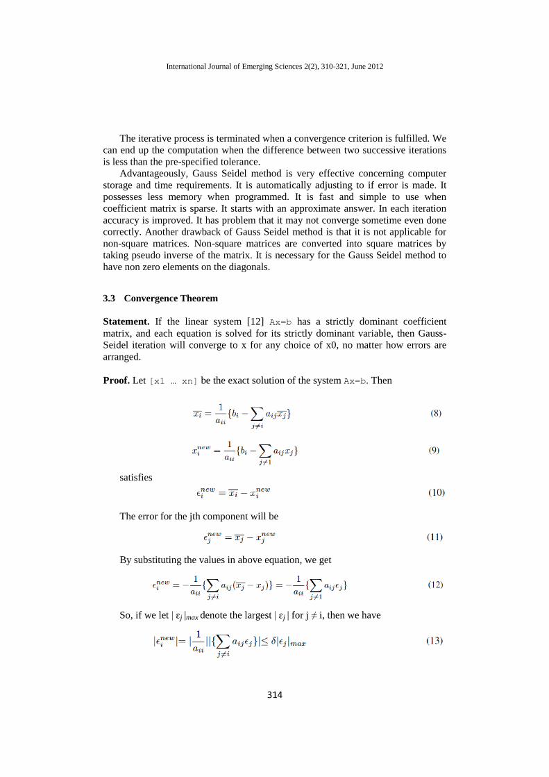
The iterative process is terminated when a convergence criterion is fulfilled. We
can end up the computation when the difference between two successive iterations
is less than the pre-specified tolerance.
Advantageously, Gauss Seidel method is very effective concerning computer
storage and time requirements. It is automatically adjusting to if error is made. It
possesses less memory when programmed. It is fast and simple to use when
coefficient matrix is sparse. It starts with an approximate answer. In each iteration
accuracy is improved. It has problem that it may not converge sometime even done
correctly. Another drawback of Gauss Seidel method is that it is not applicable for
non-square matrices. Non-square matrices are converted into square matrices by
taking pseudo inverse of the matrix. It is necessary for the Gauss Seidel method to
have non zero elements on the diagonals.
3.3 Convergence Theorem
Statement. If the linear system [12] Ax=b has a strictly dominant coefficient
matrix, and each equation is solved for its strictly dominant variable, then Gauss-
Seidel iteration will converge to x for any choice of x0, no matter how errors are
arranged.
Proof. Let [x1 … xn] be the exact solution of the system Ax=b. Then
satisfies
The error for the jth component will be
By substituting the values in above equation, we get
So, if we let | ɛj |max denote the largest | ɛj | for j ≠ i, then we have
Noreen Jamil
315
From the above equation, it is clear that the error of xinew
is smaller than the
error of other components of xnew
by a factor of at least δ. The convergence of δ will
therefore be assured if δ < 1.
3.4 Conjugate gradient Method
Conjugate gradient method [10] is a well known method for solving large number
of equations. It is efficient for the system of the form
Consider the Quadratic form:
Where A is a square, symmetric, positive definite matrix, X is a vector of
unknowns and b is a vector of right hand side values.
To minimize the function we take the derivative of that function and adjust it to
zero. After taking the derivative we have:
Since A is symmetric we can reduce the equation as
We get initial linear system by setting the derivative to zero. After that question
arises in mind that how to choose direction vectors. The good point about
Conjugate Gradient method is that it automatically generates direction vectors at the
previous step.
There are lots of iterative methods for solving optimization problems. So the
successive approximations to the solution vector A are calculated as follows
Where ρk are known as direction vectors and αk is chosen to minimize the
function in the direction of ρk. The iterative methods like Conjugate Gradient
method best suits to sparse systems. If matrix is dense then best way to solve the
system is by back substitution.
Advantageously, Conjugate Gradient method is an optimizer for all purposes
and is beneficial for high order systems as well. Like most iterative methods, exact
answer is found after finite number of steps.
International Journal of Emerging Sciences 2(2), 310-321, June 2012
316
3.5 GMRES Method
Saad introduced the GMRES method as an iterative method used for solutions of
large sparse nonsymmetric linear systems based on the Arnoldi process [23] for
computing the eigenvalues of a matrix. It computes an orthonormal basis for a
particular Krylov subspaces and solves the transforms least square problem with the
upper Hessenberg matrix. GMRES method is particularly used to minimize norm of
residual vector b – Ax.
Consider Ax = b
Where A is a non-singular matrix and b is a real n-dimensional vector. After
that we have to choose initial
guess x0 then algorithm generates approximate solution xn. Then compute r0 =
b – Ax0. Next step is to apply Arnoldi process that constructs orthonormal basis of
a space called the Krylove subspace generated by ‘A’ and r0,
Where vectors b, Ab, …, An–1b are linearly dependent, that is why Arnoldi
iteration is used to find orthonormal vectors rather than the basis q1, q2, …, qn
which form basis for kn.
After that form the approximate solution. Finally find the vector y0 that
minimizes the function.
4. ANALYSIS OF RESULTS
The efficiency of the direct and iterative methods were compared based on a 4 x 4
and a 9x 9 linear systems of equations. Then we extended it to 20 x 20 linear
systems of equations.
They are as follows
and
Noreen Jamil
317
and
International Journal of Emerging Sciences 2(2), 310-321, June 2012
318
Results produced by the three equations are given in the Tables 1, 2, 3, 4, 5 and
6.
Table 1. Linear simultaneous equations of order 4x4
Direct Method Computer Time
Gaussian Elimination 0.0567
LU-Factorization 0.0567
Table II. Linear simultaneous equations of order 4x4
Iterative Methods Number of Iterations Computer Time
Jacobi 11 0.0854
Gauss-Seidel 8 0.0567
Sor 6 0.0401
Conjugate-Gradient 3 0.0365
Generalized-Minimal-Residual 3 0.0019
5. RELATED WORK
Authors like Turner [22] faced difficulty with Gauss Elimination approach because
of round off errors and slow convergence for large systems of equations. To get rid
of these problems many authors like [10] [16] were encouraged to investigate
solutions of linear equations by indirect methods. They [11] presented comparison
of three iterative methods to solve linear systems of equations. The results shown by
[11] proved that the Successive Over-Relaxation method is faster than the Gauss
Seidel and Jacobi methods because of its performance, Number of iterations
required to converge and level of accuracy. Most of the research deal with the
iterative methods for solving linear systems of equations and inequalities for sparse
matrices. Iterative methods like [1] [13] solves linear systems of inequalities by
using relaxation method. This method states an iterative method to find a solution of
system of linear inequalities. In this iterative method, an orthogonal projection
method is connected with the relaxation method by solving one inequality at one
Noreen Jamil
319
time. Different sequential methods (derived mostly from Kaczmarz’s) have been
proposed [2]. These methods only consider one equality and inequality at a time and
each iterate is obtained from the previous iterate. Results of convergence in case of
inequality are limited to consistent systems. Cimmino [3] [5] introduced Cimmin,s
algorithm for linear equations and inequalities. By using this algorithm orthogonal
projections onto each of the violated constraints is made from the current point and
new point is taken as a convex combination of those projection points. The
algorithm is particularly appropriate to parallel implementation. Conjugate gradient
method is one of the efficient technique for solving large sparse linear systems of
equations, it involves some preconditioning techniques as well [7] [4]. In recent
years various generalizations of Conjugate Gradient method have been shown with
non-symmetric [6] [17] [9] [18] and symmetric problems [14] [15] [7] [19].
GMRES method has been presented by [20] for non-symmetric linear systems. In
this paper we compared different techniques for solving linear systems of equations.
We presented direct and iterative methods for dense and sparse linear systems and
tried to find out more efficient method for solving these linear systems.
6. DISCUSSION
The iterative methods for solving linear systems of equations have been presented
are Successive- Over Relaxation, the Gauss-Seidel method, Jacobi technique,
Conjugate Gradient and GMRES methods. In contrast the main direct methods
presented are Gaussian Elimination and LU Factorization. Three practical examples
were studied, a 4 x 4, and 9 x 9 System of linear equations, even though the
software can accommodate up to 20 x 20 system of linear equations. The analysis of
the results show that Jacobi method takes longer time 30 iterations to converge for
the 20 x 20 linear system , as compared to other methods, within the same tolerance
factor. It will also demand more computer storage to store its data. The number of
iterations differ, as that of the GMRES method has 5 iterations, whereas Conjugate
Gradient method has 17 iterations as well, Successive-Over Relaxation method, has
15 iterations, while Gauss - Seidel has 17 iterations. On contrary, in case of direct
methods, both Gaussian Elimination and LU-Factorization Method takes more time
to converge for sparse linear system as compared to dense linear system.
Results show that GMRES method requires less computer storage and is usually
faster than other direct and iterative methods. It is because iterative methods are
efficient as compared to direct methods. Lu-Decomposition method is best suited to
solve small size linear systems of equations whereas it is not suitable to solve sparse
systems because it is a direct method. That,s why indirect, iterative methods gives
the best possible solution for the problems with sparse matrices efficiently. In
summary, GMRES method is suitable for solving linear systems of equations.
Particularly, it is fitted to solve sparse matrices that arise in the application of
computer science, engineering and computer graphics. Therefore, it is most
advantageous among all iterative and direct solvers.
International Journal of Emerging Sciences 2(2), 310-321, June 2012
320
7. CONCLUSION
Different direct and iterative methods are discussed to solve linear systems of
equations. It is investigated that GMRES method is the most efficient method to
solve linear systems of equations. It requires less computational time to converge as
compared to other direct and iterative methods. Thus, the GMRES method could be
considered the more efficient one.
In future work, it would be interesting to investigate some other methods to
solve linear systems of equations. Other future directions are to investigate simple
and efficient method for solving non-linear equations.
REFERENCES
1. S. Agmon. The relaxation method for linear inequalities. Canadian Journal Mathematics,
pages 382–392, 1954.
2. Y. Censor. Row-action methods for huge and sparse systems and their applications. pages
444–466, 1981.
3. Y. Censor and T. Elfying. New methods for linear inequalities,linear algebra and its
applications. Linear Algebra and Its Applications, 64:243–253, 1985.
4. R. CHANDRA. Conjugate gradient methods for partial differential equations. Computer
Science Department, 1978.
5. A. De Pierro and A. Iuseam. A simultaneous projection method for linear inequalities.
Linear Algebra and Its Applications, 64:243–253, 1985.
6. H. C. ELMAN. Iterative methods for large sparse nonsymmetric systems of linear
equations. Computer Science Department, 1982.
7. A. L. HAGEMAN and D. M. YOUNG. Applied Iterative Methods,. Academic Press,
New York, 1981.
8. H.M.Anita. Numerical-Methods for Scientist and Engineers. Birkhauser-verlag, 2002.
9. K. C. JEA and D. M. YOUNG. Generalized conjugate gradient acceleration
ofnonsymmetrizable iterative methods. Lin. Alg. Appl, pages 159–194, 1980.
10. I. Kalambi. Solutions of simultaneous equations by iterative methods. 1998.
11. I. Kalambi. Comparison of three iterative methods for the solution of linear equations.
2008.
12. M.J.MARON. Numerical-Analysis. Collier Macmillan, 1982.
13. Motzkin and Schoenberg. The relaxation method for linear inequalities. Canadian
Journal Mathematics, pages 393–404, 1954.
14. C. C. PAIGE and M. A. SAUNDERS. Solution of sparse indefinite systems of linear
equations. SIAM J.Numer. Anal, pages 617–624, 1975.
15. B. N. PARLETT. A new look at the lanczos algorithm for solving symmetric systems of
linear equations. Lin. Alg. Appl, pages 323–346, 1980.
16. S. Rajasekaran. Numerical methods in Science and Engineering. Wheelerand Co. Ltd
Allahabad, 1992. 11
Noreen Jamil
321
17. H. C. E. S. C. EISENSTAT and M. H. SCHULTZ. Variational iterative methods for
nonsymmetric systems of linear equations. SIAM J. Numer. Anal, pages 345–357, 1983.
18. Y. SAAD. Krylov subspace methodsfor solving large unsymmetric linear systems. Math.
Comput, pages 105–126, 1981.
19. Y. SAAD. Practical use of some krylov subspace methods for solving indefinite and
unsymmetric linear systems. pages 203–228, 1984.
20. Y. SAAD and M. H. SCHULTZ. A generalized minimal residual algorithm for solving
non-symmetric linear systems. 7, 1986.
21. N. A. Saeed, A.Bhatti. Numerical Analysis. Shahryar, 2008.
22. P. Turner. Guide to Numerical Analysis. Macmillan Education Ltd. Hong Kong, 1989.
23. W.Arnoldi. The principle of minimized iteration in the solution of the matrix eigenvalue
problems. Appl.Math., pages 17–29, 1951.12