4.3 The Simplex Method and the Standard Maximization Problem Question 1: What is a standard maximization problem? Question 2: What are slack variables? Question 3: How do you find a basic feasible solution? Question 4: How do you get the optimal solution to a standard maximization problem with the Simplex Method? In Section 4.2, we examined several linear programming problems. The common theme to these problems is the number of decision variables. To be able to solve these linear programming problems graphically, they must have exactly two decision variables. In this section you will learn how to solve linear programming problems with two or more decision variables. This strategy, called the Simplex Method, will allow us to solve the problems from section 4.2 as well as other maximization problems with more than 2 variables. Since large numbers of decision variables are common in business and industry, the Simplex Method and similar variations are standard tools used to analyze linear optimization problems with hundreds of decision variables and hundreds of constraints. 1
Transcript
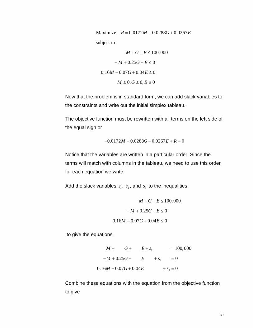
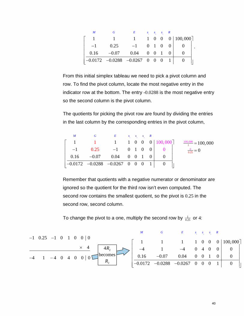
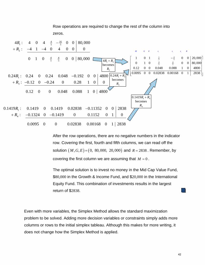
4.3 The Simplex Method and the Standard
Maximization Problem
Question 1: What is a standard maximization problem?
Question 2: What are slack variables?
Question 3: How do you find a basic feasible solution?
Question 4: How do you get the optimal solution to a standard maximization problem
with the Simplex Method?
In Section 4.2, we examined several linear programming problems. The common theme
to these problems is the number of decision variables. To be able to solve these linear
programming problems graphically, they must have exactly two decision variables.
In this section you will learn how to solve linear programming problems with two or more
decision variables. This strategy, called the Simplex Method, will allow us to solve the
problems from section 4.2 as well as other maximization problems with more than 2
variables. Since large numbers of decision variables are common in business and
industry, the Simplex Method and similar variations are standard tools used to analyze
linear optimization problems with hundreds of decision variables and hundreds of
constraints.
1
Question 1: What is a standard maximization problem?
The Simplex Method is easiest to apply to a type of linear programming problem called
the standard maximization problem.
A standard maximization problem is a type of linear
programming problem in which the objective function is to be
maximized and has the form
1 1 2 2 n nz a x a x a x
where 1, , na a are real numbers and 1, , nx x are decision
variables. The decision variables must represent non-
negative values. The other constraints for the standard
maximization problem have the form
1 1 2 2 n nb x b x b x c
where 1, , nb b and c are real numbers and 0c .
There are other types of linear programming problems (we’ll examine some of
these in the next section), but in this section all of the problems are standard
maximization problems. For instance, the craft brewery problem is a standard
maximization problem. Even though the letter describing the variable P is not the
same as z, it still fits the standard maximization form:
2
1 2
1 2
1 2
1 2
1 2
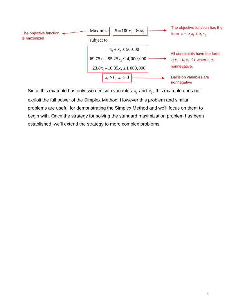
Maximize 100 80
subject to
50,000
69.75 85.25 4,000,000
23.8 10.85 1,000,000
0, 0
P x x
x x
x x
x x
x x
Since this example has only two decision variables 1x and 2x , this example does not
exploit the full power of the Simplex Method. However this problem and similar
problems are useful for demonstrating the Simplex Method and we’ll focus on them to
begin with. Once the strategy for solving the standard maximization problem has been
established, we’ll extend the strategy to more complex problems.
All constraints have the form
1 1 2 2b x b x c where c is
nonnegative.
Decision variables are nonnegative
The objective function is maximized
The objective function has the
form 1 1 2 2z a x a x
3
Question 2: What are slack variables?
The graphical strategy for solving linear programming problems relies on the idea that
the maximum value of the objective function will occur at a corner point of a bounded
feasible region. The Simplex Method is no different, but we need to work with equations
for the border of the feasible region in matrix form. The trouble is that augmented
matrices are designed to solve equations and we have inequalities. For the graphical
strategy, we simply converted each inequality to an equation. For the Simplex Method,
we’ll introduce slack variables to change the inequalities to equalities.
Let’s start from one of the linear programming problems from section 4.2:
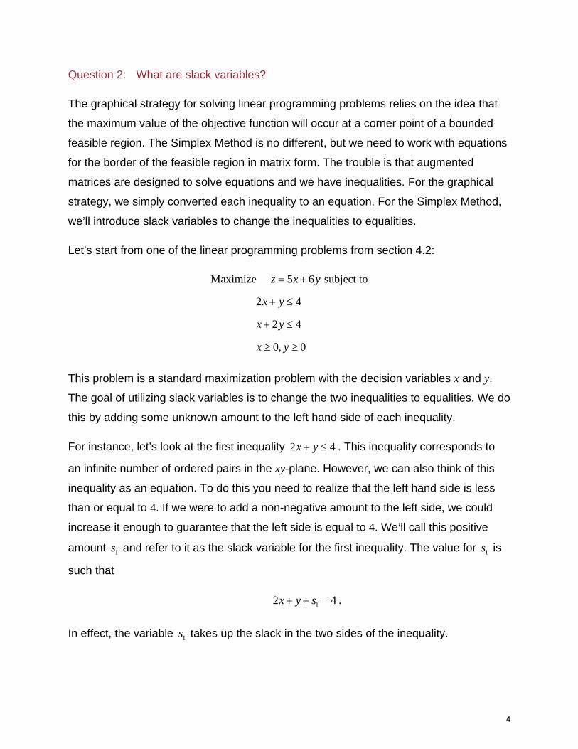
Maximize 5 6 subject to
2 4
2 4
0, 0
z x y
x y
x y
x y
This problem is a standard maximization problem with the decision variables x and y.
The goal of utilizing slack variables is to change the two inequalities to equalities. We do
this by adding some unknown amount to the left hand side of each inequality.
For instance, let’s look at the first inequality 2 4x y . This inequality corresponds to
an infinite number of ordered pairs in the xy-plane. However, we can also think of this
inequality as an equation. To do this you need to realize that the left hand side is less
than or equal to 4. If we were to add a non-negative amount to the left side, we could
increase it enough to guarantee that the left side is equal to 4. We’ll call this positive
amount 1s and refer to it as the slack variable for the first inequality. The value for 1s is
such that
12 4x y s .
In effect, the variable 1s takes up the slack in the two sides of the inequality.
4
We can apply the same reasoning to the second inequality 2 4x y . If we add a
different nonnegative amount 2s to the left side, the inequality changes to the equality
22 4x y s .
Written in this format, each inequality is now an equality with the variables (including the
slack variables) on the left side and the constant on the right side.
The objective function 5 6z x y already includes an equal sign, but not in the same
format as the equations derived from the constraints. Subtract 5x and 6y from both sides
of the objective function to put all of the variables on the left side of the equal sign. This
leaves us with the equation
5 6 0x y z .
If we put these three equations together, we get a system of three equations in five
variables. Write the constraint equations on top of the equation corresponding to the
objective function to give
1
2
2 4
2 4
5 6 0
x y s
x y s
x y z
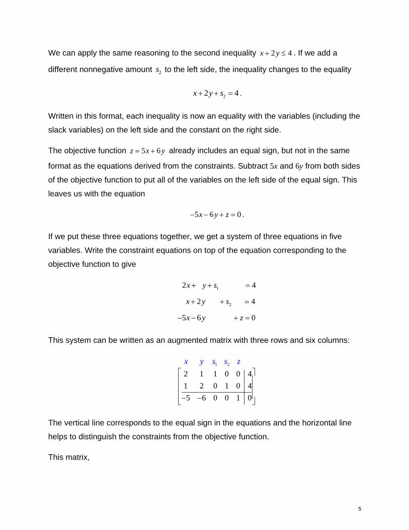
This system can be written as an augmented matrix with three rows and six columns:
1 2
2 1 1 0 0 4
1 2 0 1 0 4
5 6 0 0 1 0
x y s s z
The vertical line corresponds to the equal sign in the equations and the horizontal line
helps to distinguish the constraints from the objective function.
This matrix,
5
1 2
2 1 1 0 0 4
1 2 0 1 0 4
5 6 0 0 1 0
x y s s z
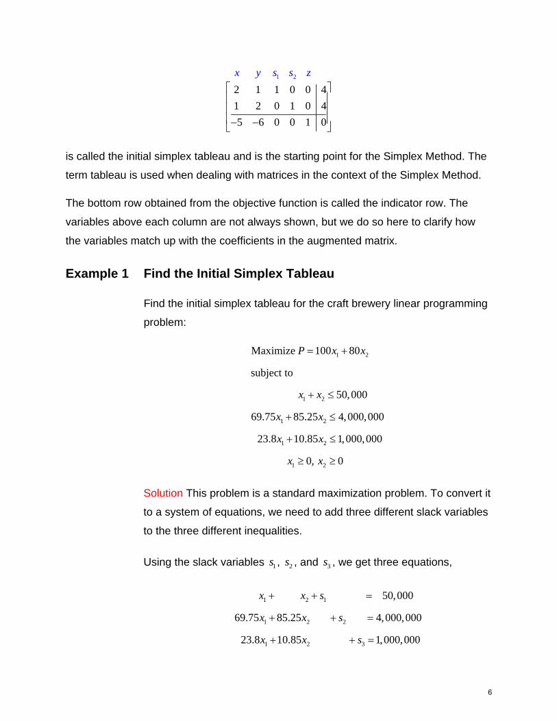
is called the initial simplex tableau and is the starting point for the Simplex Method. The
term tableau is used when dealing with matrices in the context of the Simplex Method.
The bottom row obtained from the objective function is called the indicator row. The
variables above each column are not always shown, but we do so here to clarify how
the variables match up with the coefficients in the augmented matrix.
Example 1 Find the Initial Simplex Tableau
Find the initial simplex tableau for the craft brewery linear programming
problem:
1 2
1 2
1 2
1 2
1 2
Maximize 100 80
subject to
50,000
69.75 85.25 4,000,000
23.8 10.85 1,000,000
0, 0
P x x
x x
x x
x x
x x
Solution This problem is a standard maximization problem. To convert it
to a system of equations, we need to add three different slack variables
to the three different inequalities.
Using the slack variables 1s , 2s , and 3s , we get three equations,
1 2 1
1 2 2
1 2 3
50,000
69.75 85.25 4,000,000
23.8 10.85 1,000,000
x x s
x x s
x x s
6
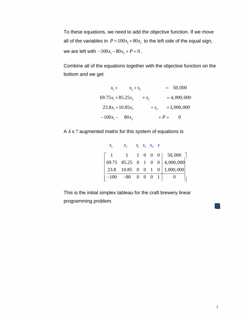
To these equations, we need to add the objective function. If we move
all of the variables in 1 2100 80P x x to the left side of the equal sign,
we are left with 1 2100 80 0x x P .
Combine all of the equations together with the objective function on the
bottom and we get
1 2 1
1 2 2
1 2 3
1 2
50,000
69.75 85.25 4,000,000
23.8 10.85 1,000,000
100 80 0
x x s
x x s
x x s
x x P
A 4 x 7 augmented matrix for this system of equations is
1 2 1 2 3
1 1 1 0 0 0 50,000
69.75 85.25 0 1 0 0 4,000,000
23.8 10.85 0 0 1 0 1,000,000
100 80 0 0 0 1 0
x x s s s z
This is the initial simplex tableau for the craft brewery linear
programming problem.
7
Question 3: How do you find a basic feasible solution?
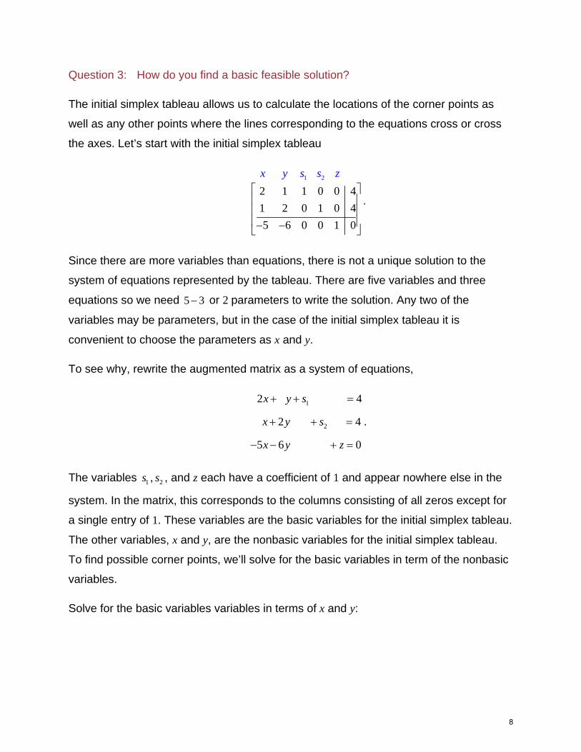
The initial simplex tableau allows us to calculate the locations of the corner points as
well as any other points where the lines corresponding to the equations cross or cross
the axes. Let’s start with the initial simplex tableau
1 2
2 1 1 0 0 4
1 2 0 1 0 4
5 6 0 0 1 0
x y s s z
.
Since there are more variables than equations, there is not a unique solution to the
system of equations represented by the tableau. There are five variables and three
equations so we need 5 3 or 2 parameters to write the solution. Any two of the
variables may be parameters, but in the case of the initial simplex tableau it is
convenient to choose the parameters as x and y.
To see why, rewrite the augmented matrix as a system of equations,
1
2
2 4
2 4
5 6 0
x y s
x y s
x y z
.
The variables 1s , 2s , and z each have a coefficient of 1 and appear nowhere else in the
system. In the matrix, this corresponds to the columns consisting of all zeros except for
a single entry of 1. These variables are the basic variables for the initial simplex tableau.
The other variables, x and y, are the nonbasic variables for the initial simplex tableau.
To find possible corner points, we’ll solve for the basic variables in term of the nonbasic
variables.
Solve for the basic variables variables in terms of x and y:
8
1
2
4 2
4 2
5 6
s x y
s x y
z x y
One possible solution to this system is found by setting the nonbasic variables x and y
equal to zero. In this situation,
1
2
4 2 0 0 4
4 0 2 0 4
5 0 6 0 0
s
s
z
.
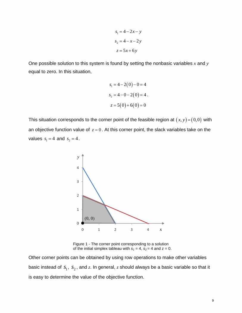
This situation corresponds to the corner point of the feasible region at , 0,0x y with
an objective function value of 0z . At this corner point, the slack variables take on the
values 1 4s and 2 4s .
Figure 1 - The corner point corresponding to a solution of the initial simplex tableau with s1 = 4, s2 = 4 and z = 0.
Other corner points can be obtained by using row operations to make other variables
basic instead of 1s , 2s , and z. In general, z should always be a basic variable so that it
is easy to determine the value of the objective function.
9
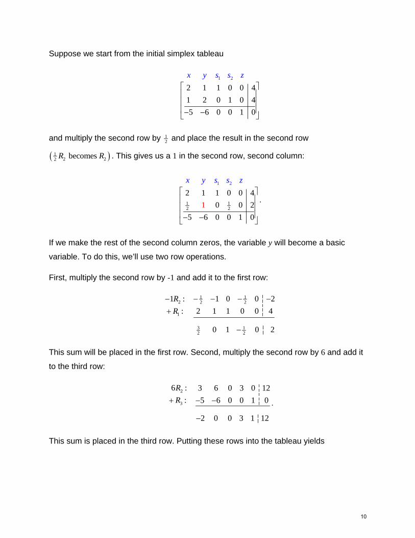
Suppose we start from the initial simplex tableau
1 2
2 1 1 0 0 4
1 2 0 1 0 4
5 6 0 0 1 0
x y s s z
and multiply the second row by 12 and place the result in the second row
12 22 becomes R R . This gives us a 1 in the second row, second column:
1 12 2
1 2
2 1 1 0 0 4
0 0 2
5 6 0 0 1 0
1
x y s s z
.
If we make the rest of the second column zeros, the variable y will become a basic
variable. To do this, we’ll use two row operations.
First, multiply the second row by -1 and add it to the first row:
1 12 2 2
1
3 12 2
1 0 0 21 :
2 1 1 0 0 4:
0 1 0 2
R
R
This sum will be placed in the first row. Second, multiply the second row by 6 and add it
to the third row:
2
3
6 : 3 6 0 3 0 12
: 5 6 0 0 1 0
2 0 0 3 1 12
R
R
.
This sum is placed in the third row. Putting these rows into the tableau yields
10
3 12 2
1 12 2
1 2
0 1 0 2
1 0 0 2
2 0 0 3 1 12
x y s s z
.
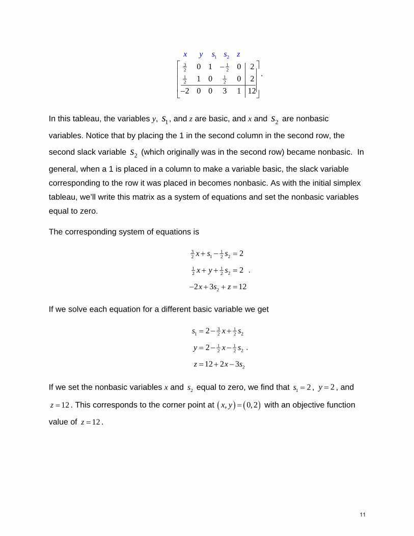
In this tableau, the variables y, 1s , and z are basic, and x and 2s are nonbasic
variables. Notice that by placing the 1 in the second column in the second row, the
second slack variable 2s (which originally was in the second row) became nonbasic. In
general, when a 1 is placed in a column to make a variable basic, the slack variable
corresponding to the row it was placed in becomes nonbasic. As with the initial simplex
tableau, we’ll write this matrix as a system of equations and set the nonbasic variables
equal to zero.
The corresponding system of equations is
3 11 22 2
1 122 2
2
2
2
2 3 12
x s s
x y s
x s z
.
If we solve each equation for a different basic variable we get
3 11 22 2
1 122 2
2
2
2
12 2 3
s x s
y x s
z x s
.
If we set the nonbasic variables x and 2s equal to zero, we find that 1 2s , 2y , and
12z . This corresponds to the corner point at , 0,2x y with an objective function
value of 12z .
11
Figure 2 - The corner point at (0,2) corresponding to s1 = 2, y = 2, and z = 12.
It is easier to find this corner point using the tableau without transforming it to a system
of equations. The key is to realize that when nonbasic variables are set equal to zero,
their coefficients in the matrix disappear. For instance, if we take the tableau we
transformed with row operations and cross out the columns of the nonbasic variables
we get:
3 12 2
1 12 2
1 2
0 1 0 2
1 0 0 2
2 0 0 3 1 12
x y s s z
By ignoring these columns, we can see that 1 2s , 2y , and 12z . Combining this
observation with our knowledge of setting the nonbasic variables equal to zero gives us
the corner point at 0,2 and objective function value 12z .
We cannot arbitrarily make a variable into a basic variable. For instance, we might make
x a basic variable by putting a 1 in the second row and first column and zeros in the rest
of the column. Starting from the original simplex tableau, we must carry out two row
operations:
12
To find the corner point corresponding to this matrix, cover the nonbasic variables and
read off the values of the basic variables:
2
1
1
0 3 1 2 0 4 4
1 2 0 1 0 4 4
0 4 0 5 1 20 20
x y s
x
z
s
s
z
Figure 3 - A solution to the tableau that is not a corner point of the feasible region.
On the surface this might not seem all that different from earlier tableaus, but this one
violates one of the assumptions for slack variables. In a standard maximization problem,
the slack variables are assumed to be non-negative. In the solution we found from this
1 2
2 1 1 0 0 4
1 2 0 1 0 4
5 6 0 0 1 0
x y s s z
1 2
0 3 1 2 0 4
1 2 0 1 0 4
0 4 0 5 1 20
x y s s z
2 1
1
2becomes
R R
R
2 3
3
5becomes
R R
R
13
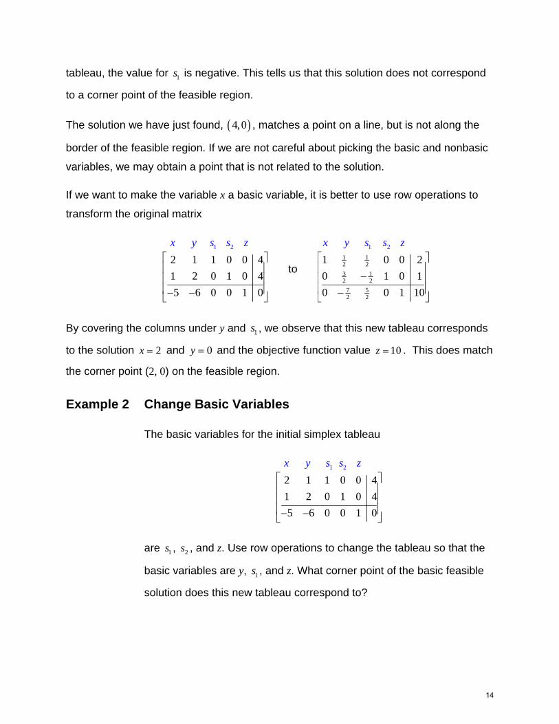
tableau, the value for 1s is negative. This tells us that this solution does not correspond
to a corner point of the feasible region.
The solution we have just found, 4,0 , matches a point on a line, but is not along the
border of the feasible region. If we are not careful about picking the basic and nonbasic
variables, we may obtain a point that is not related to the solution.
If we want to make the variable x a basic variable, it is better to use row operations to
transform the original matrix
1 2
2 1 1 0 0 4
1 2 0 1 0 4
5 6 0 0 1 0
x y s s z
to 1 12 2
1
3 12 2
2
2
7 52
1 0 0 2
0 1 0 1
0 0 1 10
x y s s z
By covering the columns under y and 1s , we observe that this new tableau corresponds
to the solution 2x and 0y and the objective function value 10z . This does match
the corner point (2, 0) on the feasible region.
Example 2 Change Basic Variables
The basic variables for the initial simplex tableau
1 2
2 1 1 0 0 4
1 2 0 1 0 4
5 6 0 0 1 0
x y s s z
are 1s , 2s , and z. Use row operations to change the tableau so that the
basic variables are y, 1s , and z. What corner point of the basic feasible
solution does this new tableau correspond to?
14
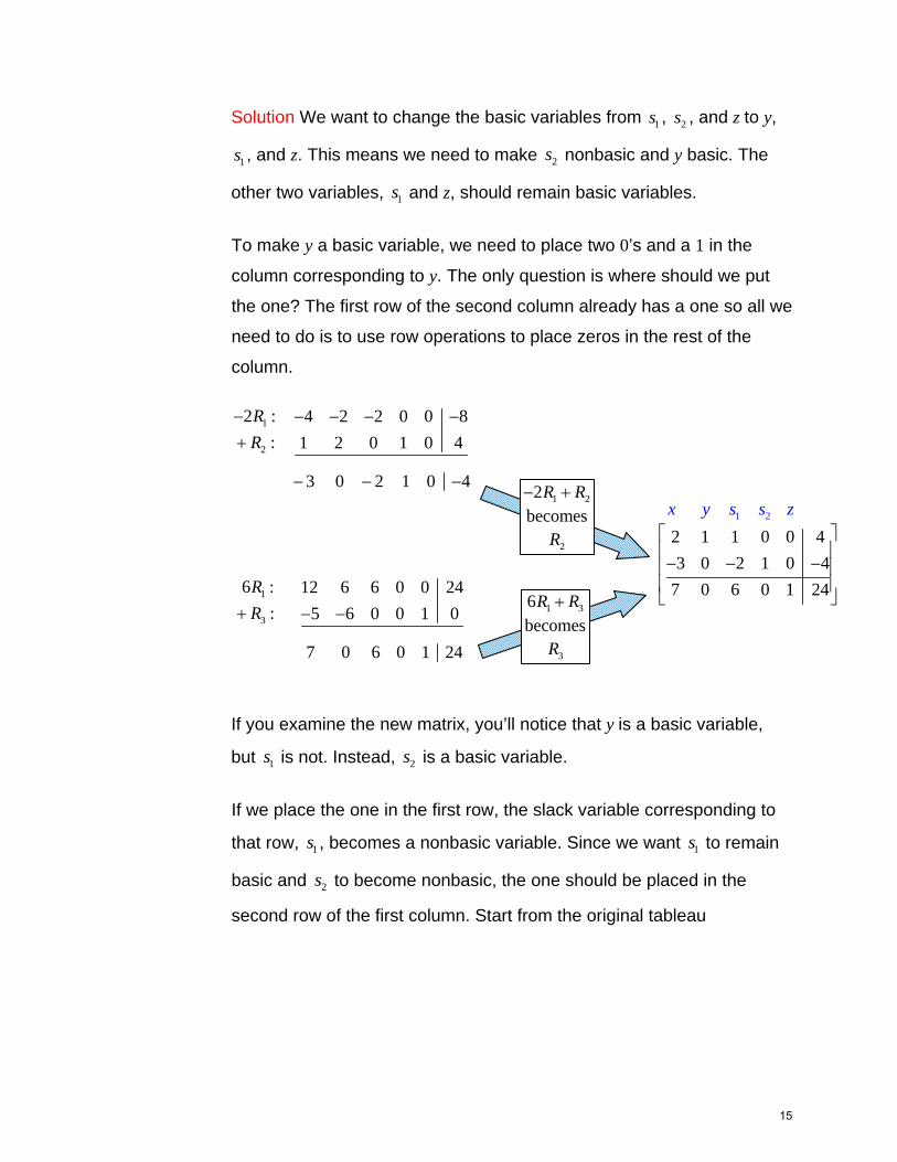
Solution We want to change the basic variables from 1s , 2s , and z to y,
1s , and z. This means we need to make 2s nonbasic and y basic. The
other two variables, 1s and z, should remain basic variables.
To make y a basic variable, we need to place two 0’s and a 1 in the
column corresponding to y. The only question is where should we put
the one? The first row of the second column already has a one so all we
need to do is to use row operations to place zeros in the rest of the
column.
If you examine the new matrix, you’ll notice that y is a basic variable,
but 1s is not. Instead, 2s is a basic variable.
If we place the one in the first row, the slack variable corresponding to
that row, 1s , becomes a nonbasic variable. Since we want 1s to remain
basic and 2s to become nonbasic, the one should be placed in the
second row of the first column. Start from the original tableau
1
2
1
3
2 : 4 2 2 0 0 8
: 1 2 0 1 0 4
3 0 2 1 0 4
6 : 12 6 6 0 0 24
: 5 6 0 0 1 0
7 0 6 0 1 24
R
R
R
R
1 2
2 1 1 0 0 4
3 0 2 1 0 4
7 0 6 0 1 24
x y s s z
1 3
3
6becomes
R R
R
1 2
2
2becomes
R R
R
15
1 2
2 1 1 0 0 4
1 2 0 1 0 4
5 6 0 0 1 0
x y s s z
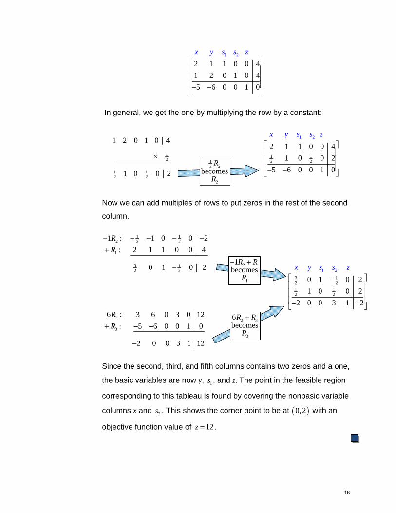
In general, we get the one by multiplying the row by a constant:
Now we can add multiples of rows to put zeros in the rest of the second
column.
Since the second, third, and fifth columns contains two zeros and a one,
the basic variables are now y, 1s , and z. The point in the feasible region
corresponding to this tableau is found by covering the nonbasic variable
columns x and 2s . This shows the corner point to be at 0,2 with an
objective function value of 12z .
1 12 2 2
1
3 12 2
2
3
1 0 0 21 :
2 1 1 0 0 4:
0 1 0 2
6 : 3 6 0 3 0 12
: 5 6 0 0 1 0
2 0 0 3 1 12
R
R
R
R
3 12 2
1 12 2
1 2
0 1 0 2
1 0 0 2
2 0 0 3 1 12
x y s s z
2 3
3
6becomes
R R
R
2 1
1
1becomes
R R
R
12 2
1
1
2
2 1 1 0 0 4
1 0 0 2
5 6 0 0 1 0
x y s s z
12
1 12 2
1 2 0 1 0 4
1 0 0 2
1
22
2
becomesR
R
16
Question 4: How do you get the optimal solution to a standard maximization problem
with the Simplex Method?
In the previous question, we learned how to make different variables into basic and
nonbasic variables. This allowed us to calculate the locations of corner points on the
feasible region and other points of intersection. For simple linear programming
problems, there can be many such points. If we naively make different variables into
basic variables, it may take a very long time to find the corner point that optimizes the
objective function.
The Simplex Method is an algorithm for solving standard maximization problems. By
following the steps below, you ensure that the points you find by changing basic
variables are corner points of the feasible region. In addition, the algorithm is iterative.
In other words, it is carried out several times with the result of each iteration providing
the starting point to the next iteration. The beauty of the Simplex Method is that each
iteration yields a larger value for the objective function and eventually leads to the
largest possible value for the objective function.
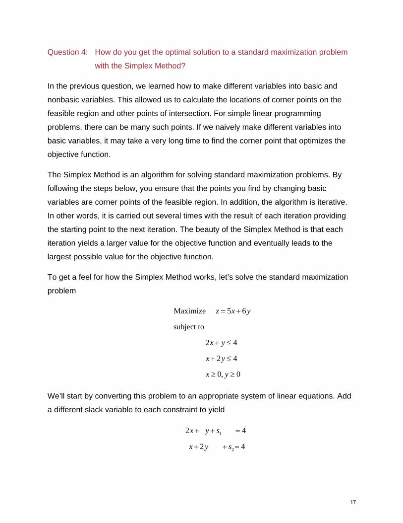
To get a feel for how the Simplex Method works, let’s solve the standard maximization
problem
Maximize 5 6
subject to
2 4
2 4
0, 0
z x y
x y
x y
x y
We’ll start by converting this problem to an appropriate system of linear equations. Add
a different slack variable to each constraint to yield
1
2
2 4
2 4
x y s
x y s
17
To convert the objective function to an appropriate form, move all of the terms with
variables to the left side of the equation. This is done by subtracting 5x and 6y from
both sides. This yields the equation 5 6 0x y z .
These equations form the system of linear equations
1
2
2 4
2 4
5 6 0
x y s
x y s
x y z
.
The augmented matrix for this system,
1 2
2 1 1 0 0 4
1 2 0 1 0 4
5 6 0 0 1 0
x y s s z
,
is the initial simplex tableau. It is the starting point for carrying out the Simplex Method
algorithm. The bottom row of the tableau is called the indicator row. The algorithm starts
by determining which variable will become a basic variable in the first iteration of the
algorithm. The variable that corresponds to the most negative entry in the indicator row
will become a basic variable.
For this matrix, the most negative entry is -6 in the second column. The variable y that
corresponds to the column will become the basic variable. This column is the pivot
column.
If we pick the column with the most negative entry in the indicator row to be the pivot
column, the objective function will increase by the largest amount. Remember, those
negative entries correspond to positive coefficients in the original objective function. For
the objective function 5 6z x y , the most negative entry in the indicator row, -6,
corresponds to the largest positive coefficient, 6, in the objective function. Increasing the
value of y in the potential solution from 0 to some positive value leads to a larger
increase in the objective function value z than increasing the value of x from 0 to the
18
same positive value. This is due to the fact that the coefficient on y is larger than the
coefficient of x. In effect, it is more efficient to change y values than x values in the
solution.
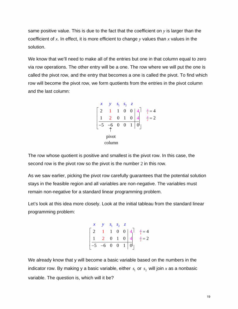
We know that we’ll need to make all of the entries but one in that column equal to zero
via row operations. The other entry will be a one. The row where we will put the one is
called the pivot row, and the entry that becomes a one is called the pivot. To find which
row will become the pivot row, we form quotients from the entries in the pivot column
and the last column:
14
2
1
4
2
2 1 0 0 4
1 0 1 0 2
5 6 0 0 1 0
pivot
co
4
l
1
umn
2 4
x y s s z
The row whose quotient is positive and smallest is the pivot row. In this case, the
second row is the pivot row so the pivot is the number 2 in this row.
As we saw earlier, picking the pivot row carefully guarantees that the potential solution
stays in the feasible region and all variables are non-negative. The variables must
remain non-negative for a standard linear programming problem.
Let’s look at this idea more closely. Look at the initial tableau from the standard linear
programming problem:
14
2
1
4
2
2 1 0 0 4
1 0 1 0 2
5 6 0
4
4
1
0
2
0 1
x y s s z
We already know that y will become a basic variable based on the numbers in the
indicator row. By making y a basic variable, either 1s or 2s will join x as a nonbasic
variable. The question is, which will it be?
19
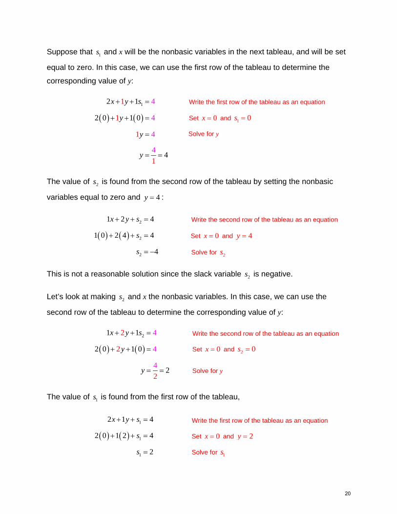
Suppose that 1s and x will be the nonbasic variables in the next tableau, and will be set
equal to zero. In this case, we can use the first row of the tableau to determine the
corresponding value of y:
1 4
4
4
4
2 1
2 0
1
1 1
1
1
0
4
x y s
y
y
y
The value of 2s is found from the second row of the tableau by setting the nonbasic
variables equal to zero and 4y :
2
2
2
1 2 4
1 0 2 4 4
4
x y s
s
s
This is not a reasonable solution since the slack variable 2s is negative.
Let’s look at making 2s and x the nonbasic variables. In this case, we can use the
second row of the tableau to determine the corresponding value of y:
21 1
2 0 1
2
2
02
4
4
42
x y s
y
y
The value of 1s is found from the first row of the tableau,
1
1
1
2 1 4
2 0 1 2 4
2
x y s
s
s
Write the first row of the tableau as an equation
Set 0x and 1 0s
Solve for y
Write the second row of the tableau as an equation
Set 0x and 4y
Solve for 2s
Write the second row of the tableau as an equation
Set 0x and 2 0s
Solve for y
Write the first row of the tableau as an equation
Set 0x and 2y
Solve for 1s
20
All variables in this case are non-negative. Note that the values for y in each case are
precisely the quotients we use to choose which row becomes the pivot row. By
choosing a value for y that is smaller (the smaller quotient), we get a situation in which
all variables are non-negative.
Now that we know that the pivot is the 2 in the second row, second column of
1 2
2 1 1 0 0 4
1 0 1 0 4
5 6 0 0 1
2
0
x y s s z
we’ll use row operations to change it to a one. The rest of the pivot column will be
changed to zeros using row operations. This change in basic variables will lead to the
largest increase in the value of the objective function and keep all variables non-
negative.
As shown in Question 3, change the pivot to a one by multiplying the second row by 12 :
Once the pivot is in place, use row operations to place zeros in the rest of the column:
122
2
becomesR
R
12
1 12 2
1 2 0 1 0 4
1 0 0 2
12 2
1
1
2
2 1 1 0 0 4
1 0 0 2
5 6 0 0 1 0
x y s s z
21
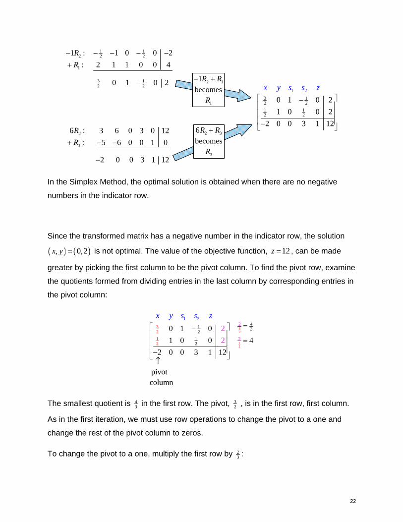
In the Simplex Method, the optimal solution is obtained when there are no negative
numbers in the indicator row.
Since the transformed matrix has a negative number in the indicator row, the solution
, 0,2x y is not optimal. The value of the objective function, 12z , can be made
greater by picking the first column to be the pivot column. To find the pivot row, examine
the quotients formed from dividing entries in the last column by corresponding entries in
the pivot column:
32
12
41
2
2
32
1
1 2
32
122
0 1 0
1 0 0 4
2 0 0 3 1 12
pivo
2
2
tcolumn
x y s s z
The smallest quotient is 43 in the first row. The pivot, 3
2 , is in the first row, first column.
As in the first iteration, we must use row operations to change the pivot to a one and
change the rest of the pivot column to zeros.
To change the pivot to a one, multiply the first row by 23 :
2 3
3
6becomes
R R
R
1 12 2 2
1
3 12 2
2
3
1 0 0 21 :
2 1 1 0 0 4:
0 1 0 2
6 : 3 6 0 3 0 12
: 5 6 0 0 1 0
2 0 0 3 1 12
R
R
R
R
3 12 2
1 12 2
1 2
0 1 0 2
1 0 0 2
2 0 0 3 1 12
x y s s z
2 1
1
1becomes
R R
R
22
To complete the transformation of the pivot column, we must use row operations to put
zeros in the rest of the pivot column:
For this tableau, the basic variables are x, y, and z. The nonbasic variables are 1s and
2s . The indicator row has no negative entries so this tableau is the final tableau. The
optimal solution is read from this tableau by setting the nonbasic variables equal to
zero.
If we cover the nonbasic variables,
2 1 43 3 3
1 2 43 3 3
74 443 3
1
3
2
1 0 0
0 1 0
0 0 1
x y s s z
,
we see that this tableau corresponds to 4 43 3, ,x y and an optimal value of 44
3z .
This is the same value we found graphically in Section 4.2
The process outlined here is summarized in the steps shown here.
11 22
2
becomes
R R
R
1 3
3
2becomes
R R
R
1 1 1 211 2 3 6 32
1 12 2 2
1 2 43 3 3
84 21 3 3 3
3
74 443 3 3
0 0:
1 0 0 2:
0 1 0
2 : 2 0 0
: 2 0 0 3 1 12
0 0 1
R
R
R
R
2 1 43 3 3
1 2 43 3 3
74 443 3
1
3
2
1 0 0
0 1 0
0 0 1
x y s s z
213
1
becomes
R
R
3 12 2
23
2 1 43 3 3
0 1 0 2
1 0 0
2 1 43 3 3
1 12 2
1 2
1 0 0
1 0 0 2
2 0 0 3 1 12
x y s s z
23
The Simplex Method
1. Make sure the linear programming problem is a standard
maximization problem.
2. Convert each inequality to an equality by adding a slack
variable. Each inequality must have a different slack
variable. Each constraint will now be an equality of the
form
1 1 2 2 n nb x b x b x s c
where s is the slack variable for the constraint. If more
than one slack variable is needed, use subscripts like
1 2, ,s s
3. Rewrite the objective function 1 1 2 2 n nz a x a x a x by
moving all of the variables to the left side. After rewriting
the equation, the function will have the form
1 1 2 2 0n na x a x a x z .
4. Convert the equations from steps 2 and 3 to an initial
simplex tableau. Put the equation from step 3 in the
bottom row of the tableau and all other equations above it.
The bottom row is called the indicator row.
5. Find the entry in the indicator row that is most negative. If
two of the entries are most negative and equal, pick the
entry that is farthest to the left. The column with this entry
is called the pivot column.
24
6. For each row except the last row, divide the entry in the
last column by the entry in the pivot column. The row with
the smallest positive quotient is the pivot row. If more than
one row has the same smallest quotient, the higher of the
rows is the pivot row.
7. The pivot is the entry where the pivot row and pivot
column intersect. Multiply the pivot row by the reciprocal
of the pivot to change it to a one.
8. To change the rest of the pivot column to zeros, multiply
the pivot row by constants and add them to the other rows
in the tableau. Replace those rows with the appropriate
sums. When complete, the pivot should be a one, and the
rest of the pivot column should be zeros.
9. If the indicator does not contain any negative entries, this
tableau corresponds to the optimum solution. In this case,
cover the nonbasic variables (set the nonbasic variables
equal to zero), and read off the solution for the basic
variables. Otherwise, repeat steps 5 through 9 until the
indicator row contains no negative numbers.
The Simplex Method will reach an optimal solution for a standard maximization problem
with any number of variables and any number of inequalities. However, problems with
large numbers of variables and inequalities may require many iterations of steps 5
through 9 to reach the optimal solution. Take special care to avoid arithmetic errors
when carrying out the row operations. A graphing calculator can make the task of
carrying out the row operations fairly painless.
25
Example 3 Find the Optimal Solution
Find the optimal solution to the linear programming problem
1 2
1 2
1 2
1 2
1 2
Maximize 2 5
subject to
2 3 15
7 6 63
5 3
0, 0
z x x
x x
x x
x x
x x
Solution Although this example has three constraints (in addition to the
non-negativity constraints), it still has two decision variables. Each
constraint needs a slack variable to convert it to an equation. Using the
slack variables 1s , 2s , and 3s , the constraints become
1 2 1
1 2 2
1 2 3
2 3 15
7 6 63
5 3
x x s
x x s
x x s
Move all of the variable terms in the objective function to the left side of
the equation to yield
1 22 5 0x x z
These equations become the initial simplex tableau
1 2 1 2 3
2 3 1 0 0 0 15
7 6 0 1 0 0 63
1 5 0 0 1 0 3
2 5 0 0 0 1 0
x x s s s z
26
The bottom row of the initial simplex tableau is the indicator row. The
most negative entry of the indicator row is -5. This means the pivot
column is the second column in the tableau.
To determine the pivot row, compute the quotients formed by dividing
entries in the last column by entries in the pivot column,
1 2 1 2 3
15
63
3
6
2 1 0 0 0 57 0 1 0 0 10.51 5 0 0 1 0 3
2 5 0 0 0 1 0
3
6
15
63
x x s s s z
Any negative quotients, such as 35 in the third row, are discarded. The
quotient formed in the first row, 153 , is the smallest quotient so the pivot
is the 3 in the first row, second column.
In the first iteration of the simplex method, we must use row operations
to change the pivot to a one and all other entries in the pivot column to
zero.
The pivot is changed to a one by multiplying the first row by 13 . Carrying
out the row operation yields
Three row operations are necessary to put the zeros in the rest of the
pivot column:
113
1
becomes
R
R
13
2 13 3
2 3 1 0 0 0 15
1 0 0 0 5
1 2 1 2 3
2 13 31 0 0 0 5
7 6 0 1 0 0 63
1 5 0 0 1 0 3
2 5 0 0 0 1 0
x x s s s z
27
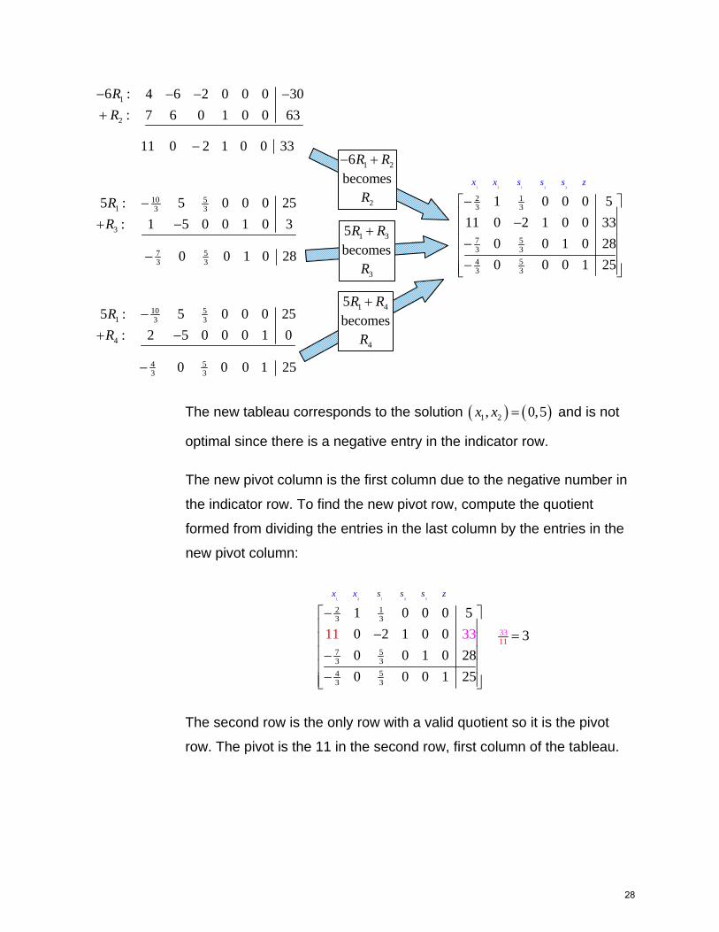
The new tableau corresponds to the solution 1 2, 0,5x x and is not
optimal since there is a negative entry in the indicator row.
The new pivot column is the first column due to the negative number in
the indicator row. To find the new pivot row, compute the quotient
formed from dividing the entries in the last column by the entries in the
new pivot column:
1 2 1 2 3
2 13 3
7 53 3
543 3
3311
1 0 0 0 5
0 2 1 0 0 3
0
33
0 1 0 28
0 0 0 1 25
11
x x s s s z
The second row is the only row with a valid quotient so it is the pivot
row. The pivot is the 11 in the second row, first column of the tableau.
1 2
2
6becomes
R R
R
1 3
3
5becomes
R R
R
1 4
4
5becomes
R R
R
1
2
10 51 3 3
3
7 53 3
10 51 3 3
4
543 3
6 : 4 6 2 0 0 0 30
: 7 6 0 1 0 0 63
11 0 2 1 0 0 33
5 : 5 0 0 0 25
: 1 5 0 0 1 0 3
0 0 1 0 28
5 0 0 0 255 :
2 5 0 0 0 1 0:
0 0 0 1 25
R
R
R
R
R
R
1 2 1 2 3
2 13 3
7 53 3
543 3
1 0 0 0 5
11 0 2 1 0 0 33
0 0 1 0 28
0 0 0 1 25
x x s s s z
28
Multiply the pivot row by 111 to change the pivot to a one:
To complete this Simplex Method iteration, we must place zero above
and below the pivot using row operations.
Three row operations are required to place the zeros above and below
the pivot.
The indicator row does not contain any negative numbers so the
optimal solution has been reached.
The solution to the linear programming problem is easily observed by
covering the columns corresponding to the nonbasic variables 1s and 2s
:
22 13
1
becomes
R R
R
72 33
3
becomes
R R
R
42 43
4
becomes
R R
R
2 4 222 3 33 333
2 11 3 3
7 233 33
7 71472 3 33 333
7 53 3 3
74133 33
84 442 3 33 333
544 3 3
47 433 33
0 0 0 2:
1 0 0 0 5:
0 1 0 0 7
0 0 0 7:
0 0 1 0 28:
0 0 1 0 35
0 0 0 4:
0 0 0 1 25:
0 0 0 1 29
R
R
R
R
R
R
1 2 1 2 3
7 233 33
2 111 11
74133 33
47 433 33
0 1 0 0 7
1 0 0 0 3
0 0 1 0 35
0 0 0 1 29
x x s s s z
1211
2
becomes
R
R
111
2 111 11
11 0 2 1 0 0 33
1 0 0 0 3
1 2 1 2 3
2 13 3
2 111 11
7 53 3
543 3
1 0 0 0 5
1 0 0 0 3
0 0 1 0 28
0 0 0 1 25
x x s s s z
29
1 2 1 2 3
7 233 33
2 111 11
74133 33
47 433 33
0 1 0 0 7
1 0 0 0 3
0 0 1 0 35
0 0 0 1 29
x x s s s z
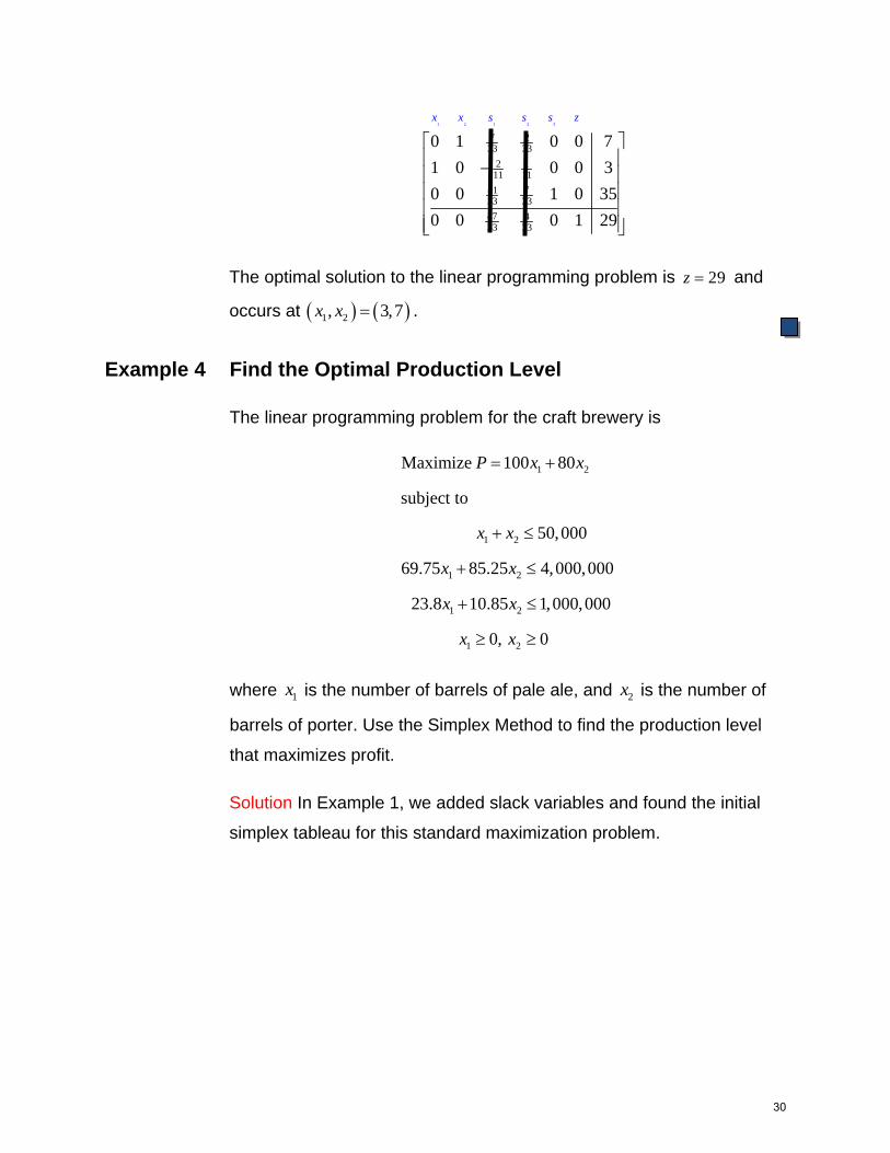
The optimal solution to the linear programming problem is 29z and
occurs at 1 2, 3,7x x .
Example 4 Find the Optimal Production Level
The linear programming problem for the craft brewery is
1 2
1 2
1 2
1 2
1 2
Maximize 100 80
subject to
50,000
69.75 85.25 4,000,000
23.8 10.85 1,000,000
0, 0
P x x
x x
x x
x x
x x
where 1x is the number of barrels of pale ale, and 2x is the number of
barrels of porter. Use the Simplex Method to find the production level
that maximizes profit.
Solution In Example 1, we added slack variables and found the initial
simplex tableau for this standard maximization problem.
30
The initial simplex tableau is a 4 x 7 matrix,
1 2 1 2 3
1 1 1 0 0 0 50,000
69.75 85.25 0 1 0 0 4,000,000
23.8 10.85 0 0 1 0 1,000,000
100 80 0 0 0 1 0
x x s s s P
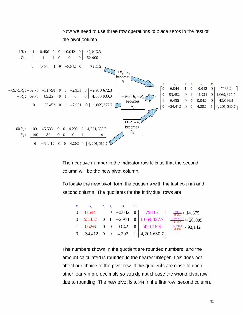
The most negative entry in the indictor row is -100. This entry means the
pivot column is the first column in the tableau. The quotients formed