24
45 8 Population Projections (policy analysis) Fish 458; Lecture 21
| Date post: | 20-Dec-2015 |
| Category: |
Documents |
| View: | 231 times |
| Download: | 0 times |

458
Population Projections(policy analysis)
Fish 458; Lecture 21

458
Policy Evaluation-I It is often the objective for developing and
fitting a model is to address “what if” questions. What is the impact of: removal limits (quotas: individual / Olympic); time / area closures; gear restrictions (number of pots, traps,
gillnets); bag limits; minimum / maximum sizes; and vessel numbers / size of vessels.
458
Policy Evaluation - II We are often not looking for optimal
policies. Rather, we want to identify polices that are robust to: Estimation error. Uncertainty regarding the true model. Implementation uncertainty. Environmental variability and environmental
change. “Optimal policies” can often be found if
we know the true model but these may perform poorly if applied to the wrong model.

458
Policy Evaluation-III(objectives and tactics)
Policies are based on choosing tactics (quotas, minimum sizes, closed areas) to achieve management objectives / goals.
Corollary - if we don’t know the management objectives we cannot (sensibly) compare different policies.
Problem: often the decision makers have not agreed on any objectives (or are unwilling to state their actual objectives publicly).

458
Policy Evaluation-IV(objectives and tactics)
We distinguish between high-level objectives (e.g. conserve the stock) and operational (quantitative) objectives (the probability of dropping below 0.1K should not be greater than 0.1 over a 20-year period).
Many decision makers confuse the tactics (what to do next year) with the objectives (why are we doing what we are doing next year).

458
Objectives for Fisheries Management
(typical high-level objectives)
High level objectives arise from: National legislation (MMPA,
Magnusson-Stevens Act, ESA). International Agreements (CCAMLR,
IWC, UN Fish Stocks Agreement). Court decisions.

458
Objectives for Fisheries Management
(Objectives for commercial whaling)
1. Acceptable risk level that a stock not be depleted (at a certain level of probability) below some chosen level (e.g. some fraction of its carrying capacity), so that the risk of extinction of the stock is not seriously increased by exploitation;
2. Making possible the highest continuing yield from the stock; and
3. Stability of catch limits.
The first objective was assigned highest priority but was not fully quantified.

458
Objectives for Fisheries Management(Australian Fisheries Management
Authority)
1. Implementing efficient and cost-effective fisheries management on behalf of the Commonwealth;
2. Ensuring that the exploitation of fisheries resources and the carrying on of any related activities are conducted in a manner consistent with the principles of ecologically sustainable development and the exercise of the precautionary principle;
3. aximising economic efficiency in the exploitation of fisheries resources;
4. nsuring accountability to the fishing industry and to the Australian community; and
5. Achieving government targets in relation to the cost recovery.

458
Operational and High-level objectives
Operational objectives describe the high-level objectives quantitatively.
Preserve biodiversity (have at least 80% of all species protected in a system of reserves).
Protect endangered species (have an 80% probability that all currently endangered species are no longer endangered within 50 years).
Protect ecosystem functioning (who knows what exactly what this means??)

458
Techniques for Policy Evaluation
We can sometimes evaluate the implications of a policy analytically (e.g. the impact of changes in fishing intensity on yield-per-recruit).
More commonly, we have to evaluate policy alternatives using Monte Carlo simulation methods.
Specify the high-level management objectives. Specify the operational management objectives. Develop models of the system to be managed (including
their uncertainty). Use simulation to determine the implications of each
policy. Summarize the results.

458
Projecting Forward - I
1. Define the state of the system in the first year of the projection.
2. Calculate the catch limit based on the current state of the system.
3. Project ahead one year (there may be implementation error at this stage) and update the dynamics.
4. Repeat steps 2-3 for each future year. 5. Repeat steps 1-4 many times.

458
The Simplest Decision Rules
Constant catch (b=0). Constant harvest rate (a=0).
Constant escapement (a<0).
Catch Stocksizea b

458
The Simplest Decision Rules
0
2
4
6
8
10
12
14
0 0.25 0.5 0.75 1
Population Size
Ca
tch
Lim
it
(a=10,b=0)
Catch Stocksizea b
(a=0,b=10)
(a=-2.5,b=12.5)

458
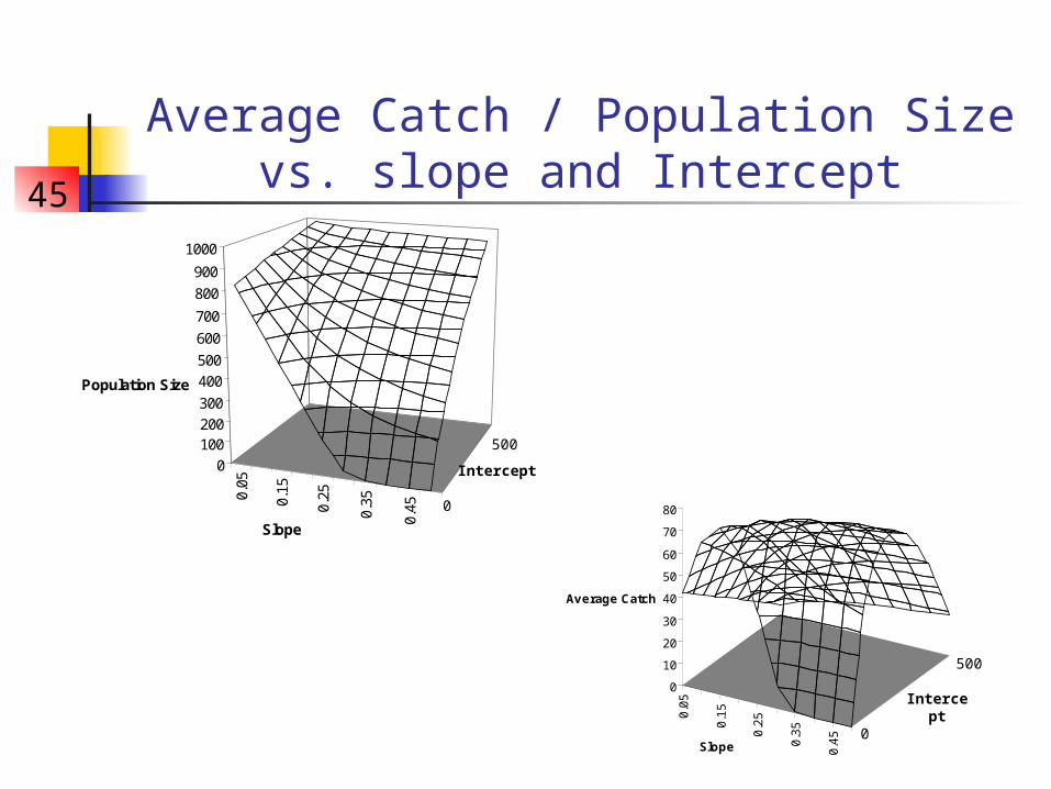
Evaluating the Simplest Rule
Model of the state of the system (Schaefer model):
This a deterministic model so we only have to do a single simulation as there is no uncertainty.
1 0(1 / ) ; 0.2t t t t t
t t
B B r B B K C B K
C a bB
458
0.0
5
0.1
5
0.2
5
0.3
5
0.4
5
0
10
20
30
40
50
60
70
80
Average Catch
Slope
0.05
0.15
0.25
0.35
0.45
0
100200
300
400
500
600
700
800
900
1000
Population Size
Slope
Average Catch / Population Sizevs. slope and Intercept
Intercept
0
500
0
500
Intercept
458
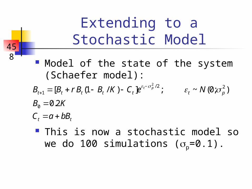
Extending to a Stochastic Model
Model of the state of the system (Schaefer model):
This is now a stochastic model so we do 100 simulations (p=0.1).
2 / 2 21
0
[ (1 / ) ] ; ~ (0; )
0.2
t p
t t t t t t p
t t
B B r B B K C e N
B K
C a bB

458
Catch and Population Size Trajectories
0.0
100.0
200.0
300.0
400.0
500.0
600.0
700.0
0 6 12 18 24 30 36 42 48 54 60 66 72 78 84 90 96
Year
Catch
Population Size

458
Average Catch / Population Size / CVvs. slope and Intercept
0.0
5
0.1
5
0.2
5
0.3
5
0.4
5
0
10
20
30
40
50
60
70
80
Average Catch
Slope
Intercept
0
500
0.05
0.15
0.25
0.35
0.45
0
100200
300
400
500
600
700
800
900
1000
Population Size
Slope
Intercept
0
500
0.05
0.15
0.25
0.35
0.45
0
0.1
0.2
0.3
0.4
0.5
0.6
CV
Slope
0
500
Intercept
Between simulation CVof average catch

458
Average catch vs. Population Size
0
200
400
600
800
1000
1200
0 20 40 60 80
Average catch
Po
pu
latio
n S
ize

458
CV of catch vs. Average Catch
0
0.2
0.4
0.6
0.8
0 20 40 60 80
Average catch
CV
of
Ca
tch

458
Allowing for Errors in Stock Assessment
We now allow for correlated errors when conducting assessments (if this year’s assessment is wrong, next year’s is also likely to be wrong) :
This approach to modeling assessment errors ignores biases in assessment results – also assessment errors are unlikely to be log-normally distributed.
2
2
/ 2 21
0
/ 2 2 21 1
[ (1 / ) ] ; ~ (0; )
0.2
; 1 ; ~ (0; )
t p
t p
t t t t t t p
t t t t t t e
B B r B B K C e N
B K
C a bB e z z N

458
0.0
5
0.1
0.1
5
0.2
0.2
5
0.3
0.3
5
0.4
0.4
5
0.5
0
0.2
0.4
0.6
0.8
1
1.2
1.4
AAV
Slope
Intercept
0
500
Allowing for Errors in Stock Assessment
0.0
5
0.1
0.1
5
0.2
0.2
5
0.3
0.3
5
0.4
0.4
5
0.5
0
0.2
0.4
0.6
0.8
1
1.2
1.4
1.6
AAV
Slope
Intercept
0
500
Measuring the within-year variance in catches:1| | /y y y
y y
AAV C C C
No Stock Assessment Errors With Stock Assessment Errors

458
Going Beyond the Simple Case
Rather than assume assessment errors are log-normally distributed, simulate the process of conducting annual assessments (this is highly computationally intensive).
Examine strategies designed to achieve specific management objectives (e.g. select catch limits so that the probability of recovery equals a desired level).

458
Readings Burgman et al. (1993); Chapter 3. Hilborn and Walters (1992);
Chapters 15-18. Quinn and Deriso (1999); Chapter
11.


![Chapter 458-61A Chapter 458-61A WAC REAL …lawfilesext.leg.wa.gov/law/WACArchive/2013/WAC-458-61A...458-61A-101 Real Estate Excise Tax [Ch. 458-61A WAC—p. 2] (8/3/11) Legislation](https://static.documents.pub/doc/80x56/5fb4b3e18aff3f19c748349f/chapter-458-61a-chapter-458-61a-wac-real-458-61a-101-real-estate-excise-tax.jpg)
