HAL Id: hal-00554879https://hal.archives-ouvertes.fr/hal-00554879v2

Submitted on 27 Mar 2012

HAL is a multi-disciplinary open accessarchive for the deposit and dissemination of sci-entific research documents, whether they are pub-lished or not. The documents may come fromteaching and research institutions in France orabroad, or from public or private research centers.

L’archive ouverte pluridisciplinaire HAL, estdestinée au dépôt et à la diffusion de documentsscientifiques de niveau recherche, publiés ou non,émanant des établissements d’enseignement et derecherche français ou étrangers, des laboratoirespublics ou privés.

4D imaging of fracturing in organic-rich shales duringheating

Maya Kobchenko, Hamed Panahi, Francois Renard, Dag Kristian Dysthe,Anders Malthe-Sorenssen, Adriano Mazzini, Julien Scheibert, Bjorn Jamtveit,

Paul Meakin

To cite this version:Maya Kobchenko, Hamed Panahi, Francois Renard, Dag Kristian Dysthe, Anders Malthe-Sorenssen,et al.. 4D imaging of fracturing in organic-rich shales during heating. Journal of Geophysical Research,American Geophysical Union, 2011, 116, pp.B12201. �10.1029/2011JB008565�. �hal-00554879v2�

1

4D imaging of fracturing in organic-rich shales during heating 1

2

Maya Kobchenko1, Hamed Panahi

1,2, François Renard

1,3, Dag K. Dysthe

1, Anders Malthe-3

Sørenssen1, Adriano Mazzini

1, Julien Scheibert

1,4, Bjørn Jamtveit

1 and Paul Meakin

1,5,6 4

5

1 Physics of Geological Processes, University of Oslo, Norway

6

2 Statoil ASA, Oslo, Norway

7

3 Institut des Sciences de la Terre, Université Joseph Fourier and CNRS, Grenoble, France

8

4 Laboratoire de Tribologie et Dynamique des Systèmes, CNRS, Ecole Centrale de Lyon, Ecully CEDEX, 9

France. 10

5 Idaho National Laboratory, Idaho Falls, USA

11

6 Institute for Energy Technology, Kjeller, Norway

12

13

2

Abstract 14

To better understand the mechanisms of fracture pattern development and fluid escape in 15

low permeability rocks, we performed time-resolved in situ X-ray tomography imaging to 16

investigate the processes that occur during the slow heating (from 60° to 400°C) of organic-rich 17

Green River shale. At about 350°C cracks nucleated in the sample, and as the temperature 18

continued to increase, these cracks propagated parallel to shale bedding and coalesced, thus 19

cutting across the sample. Thermogravimetry and gas chromatography revealed that the 20

fracturing occurring at ~350°C was associated with significant mass loss and release of light 21

hydrocarbons generated by the decomposition of immature organic matter. Kerogen 22

decomposition is thought to cause an internal pressure build up sufficient to form cracks in the 23

shale, thus providing pathways for the outgoing hydrocarbons. We show that a 2D numerical 24

model based on this idea qualitatively reproduces the experimentally observed dynamics of crack 25

nucleation, growth and coalescence, as well as the irregular outlines of the cracks. Our results 26

provide a new description of fracture pattern formation in low permeability shales. 27

28

Key words: primary migration, shale, X-ray computed micro-tomography, kerogen, 29

hydrocarbon, reaction fracturing 30

31

3

1. Introduction 32

A wide variety of geological phenomena involve the generation and migration of fluids in 33

low permeability rocks. For example, dehydration of sediments in subduction zones generates 34

large fluxes of water that rise along low-permeability subduction interfaces, and provide a 35

mechanism for creep and/or slow earthquakes [Obara, 2002]. Similarly, the illitization of clays 36

at depth and the production of methane in organic-rich shales were suggested to contribute to the 37

development of overpressure and the formation of piercement structures, which are manifest on 38

the surface as mud volcanoes [Mazzini et al, 2009]. Also, the emplacement of magmatic bodies 39

into sedimentary basins induces rapid decomposition of organic matter, and the resulting gases 40

migrate through low permeability rocks in quantities that may significantly alter the climate 41

[Svensen et al., 2004]. In all these geological systems, the migration of a fluid through low 42

permeability rocks is coupled with deformation. This type of coupling between fluid flow and 43

deformation is also important in the primary migration of hydrocarbons. 44

Primary migration is the transport of hydrocarbon fluids from extremely low permeability 45

source rocks, in which they are generated, to more permeable rocks through which they migrate 46

to a trap (reservoir) or to the surface. This natural process is of both economic and fundamental 47

interest. As the organic-rich fine grained sediment from which the source rock is formed is 48

buried, the organic material is transformed into complex high molecular weight/cross-linked 49

organic oil and gas precursors (kerogen). As the burial depth increases, the temperature and 50

pressure rise, and kerogen decomposes into low molecular weight hydrocarbon fluids (gas and 51

oil), which have much lower viscosities than the kerogen. The generated hydrocarbon fluids 52

escape from the shale into secondary migration pathways, by processes that remain enigmatic, in 53

spite of decades of investigation [Bjørlykke, 2010]. 54

4

Fracturing is commonly cited as a likely mechanism to increase the permeability of 55

source rocks and provide pathways for the generated hydrocarbons [Berg and Gangi, 1999; Lash 56

and Engelder, 2005]. During kerogen decomposition, generation of less dense fluids leads to 57

pore-pressure build-up, which may cause fracturing of the host rock. The presence of 58

microcracks is commonly observed in thin sections of recovered source rock samples [Capuano, 59

1993; Vernik, 1993; Marquez and Mountjoy, 1996; Lash and Engelder, 2005], suggesting that 60

microcracks may be involved in fluid migration. 61

Under natural conditions, this fracture process takes place at depths of several kilometers 62

over millions of years, making its monitoring impossible. Therefore, it is very important to 63

construct adequate models of primary migration. Several theoretical and numerical studies of 64

fracture formation in organic-rich shales have been described in the scientific literature [Ozkaya, 65

1988; Jin et al., 2010]. Jin et al. [2010] introduced a fracture mechanics model of subcritical 66

crack propagation and coalescence, based on the assumption of linear elastic behavior of the 67

rock. Although the model provides an estimate of the fracture propagation time, the 3D geometry 68

and mechanism of fracture formation in heterogeneous shale remain unclear. 69

To better understand the complex phenomenon of hydrocarbon expulsion from very low 70

permeability source rock, we employed a new experimental approach – real-time 3D X-ray 71

tomography – during gradual heating of a shale sample coupled with thermogravimetry and 72

petrography analyses before and after heating. This study included only unconfined samples, but 73

it is an important step towards the goal of unraveling the numerous and complex mechanisms 74

controlling primary migration. 75

2. Characterization of Green River Shale samples 76

5

The samples were obtained from an outcrop of the organic-rich R-8 unit of the Green 77

River Shale Formation (Piceance Basin, northwestern Colorado, USA). The formation consists 78

of Eocene lacustrine marl/silt sediments [Ruble et al., 2001] with well-developed lamination and 79

anisotropic mechanical properties [Vernik and Landis, 1996]. It contains organic matter (total 80

organic content = 9.92 wt% in analyzed samples) present in the form of patches of kerogen, 81

preferentially distributed parallel to the bedding (Figure 1A, B). This part of the formation has 82

never been buried deeply enough to reach temperatures sufficient to cause significant thermal 83

maturation. 84

Cylindrical core samples (5mm height, 5mm in diameter) cut perpendicular to the 85

bedding were prepared for X-ray tomography. Thin sections were taken before and after heating. 86

Optical microscope images (Figure 1A, B) highlight the micro-fabric of the uncooked shale 87

consisting of alternating lamellae of: coarser and lighter colored carbonate cemented layers rich 88

in siliciclastic grains (e.g. quartz) and pyrite framboids; and darker and finer grained clay-rich 89

layers, containing greater amount of discontinuous organic matter lenses. 90

3. 4D imaging and data processing 91

Time-lapse X-ray tomography 3D imaging of the shale samples was carried out using 92

beamline ID19 at the European Synchrotron Radiation Facility in Grenoble, France. This non-93

invasive imaging technique measures the absorption of X-rays, to produce a 3D attenuation map. 94

The prepared shale cylinder was placed in a home-built furnace in contact with air, with 95

no confining pressure, and it was gradually heated in-situ from 60°C to 400°C at approximately 96

1°C/min. 68 3D scans of this sample were taken, of which 28 were acquired during the heating 97

phase and the rest at 400°C. For all scans, 1500 radiographs were acquired while the sample was 98

rotated over 180°. The beam energy of 20 keV allowed images to be captured with a spatial 99

6

resolution of 5 µm (5x5x5µm3 voxels) and a time resolution of 11-14 minutes per 3D scan. 3D 100

raw-tomograms representing the microporous structure of the sample at different stages of 101

heating were constructed from the X-ray data. The final volumes contained 8303 voxels coded in 102

8-bit gray levels. 103

The 3D images were processed in two ways. First, the strain field was measured in a 104

typical 2D vertical slice of the volume, using digital image correlation [Rechenmacher and 105

Finno, (2004); Hild and Roux, 2006; Viggiani, (2009); Bornert et al, 2010]. Second, in order to 106

determine crack geometries and track crack propagation, the shape, volume and morphology of 107

the cracks were analyzed in 3D using the AvizoFire© software package. Quantitative analysis of 108

the crack formation required isolation of the cracks from the rock matrix. Due to the small crack 109

opening (4-5 voxels), the following procedure was applied: firstly a binary mask was used to 110

delete the background; then an edge-preserving smoothing filter based on Gaussian smoothing 111

combined with a non-linear diffusion algorithm was applied; then a “watershed” procedure 112

enabled individual cracks to be isolated [Sonka et al, 1999]. The final result of this segmentation 113

procedure was a series of cracks consisting of connected voxels, marked by different 114

labels/colors (Figure 2A). 115

4. Observation of deformation and crack formation 116

Correlation analysis and 3D image analysis were performed to determine the deformation 117

of the sample before fracturing and the geometries of the developing cracks. The spatial 118

fluctuations of the attenuation maps (see Figure 2B) served as markers when the digital 119

correlation technique was used to compare successive images. To calculate the correlation matrix 120

we used a correlation box of size 25 by 25 pixels (125 by 125 µm2), which enabled us to measure 121

the spatial distribution of micro-displacements. 122

7

Between room temperature and 300°C, the shale dilated anisotropically in the vertical 123

(perpendicular to the shale bedding) and horizontal (parallel to the shale bedding) directions, and 124

the strain curves showed a quasi-linear increase with temperature, as expected for linear thermal 125

expansion (Figure 3A). The coefficient for thermal expansion was determined to be 5.5*10-5

/°C 126

in the vertical direction and 2.5*10-5

/°C in the horizontal direction, which clearly indicates the 127

anisotropy of the shale, in agreement with other studies on the same shale [Grebowicz, 2008]. At 128

300°C, the vertical expansion started to deviate from linearity, which is likely related to the onset 129

of organic degassing before crack formation. At a temperature of about 350°C the sample 130

undergoes rapid localized deformation owing to fluid generation and the onset of fracturing. The 131

sample breaks, black structures corresponding to the newly formed cracks appear in the images 132

(see Figure 2B), which have no equivalent in the preceding ones, thus ruining the correlation 133

technique. Moreover, after the sample fractures, global movement of the sample occurs 134

(translation and rotation), with displacements from one data set to the next of amplitude greater 135

than 12 pixels, which was estimated to be the maximum displacement that can be accurately 136

measured using the correlation technique. Even though the correlation results during and after 137

fracturing are not trustworthy, this technique accurately determines the sample deformation 138

before fracturing occurs. 139

With 3D tomography, we imaged 3 stages of fractures propagation. The first 140

microfracture pattern was detected at a temperature of about 350°C. Figure 2A shows a 3D 141

rendering of the most opened fractures at T=391°C (third time step) and Figures 2B and 2C show 142

a vertical slice through the tomography image. The general direction of crack propagation 143

followed the shale bedding, and no perpendicular fractures were observed (Figure 2B). Pyrite 144

8

grains, observable as bright spots in the tomography images (Figure 2C), affected crack growth 145

by pinning the crack front, and controlling the out-of-plane fluctuations of the crack path. 146

The fractures can be described in terms of two rough, essentially parallel surfaces that 147

enclose the fracture aperture. Both surfaces can be described by height functions, h1(x,y) and 148

h2(x,y), where (x,y) is the position in the common plane. Figure 4A shows the topography of 149

fracture surface h1(x,y), where the fluctuation of surface function h1(x,y) around the flat plane 150

(x,y) is indicated by the color code. Cracks have essentially constant aperture widths - the 151

thickness function h2(x,y) - h1(x,y) (4-5 pixels, i.e. 20-25 micrometers, see Figure 4B), and rough 152

irregular outlines. The amplitude of the topography variation is around 10-15 pixels (i.e. 50-75 153

micrometers), as seen in the Figure 4A. The mid-plane (H(x,y) = [h1(x,y) + h2(x,y)]/2) is also 154

rough, and it fluctuates about a flat plane – the “plane of the fracture”. The projections of h1(x,y), 155

h2(x,y) and ([h1(x,y) + h2(x,y)]/2 into this plane, in a direction perpendicular to the plane, have a 156

common shape, which consists of a continuous region with rough edges. When one fracture 157

coalesces with another, a new fracture is formed, and it can be described in terms of the rough 158

surfaces Hnew

(x,y), h1new

(x,y) and h2new

(x,y). The projections of these rough surfaces are also a 159

common shape, which consists of a continuous region with rough edges. The planes of the 160

coalesced fracture and the two fractures that coalesced to form it are more-or-less parallel, and 161

also quasi-parallel to the shale lamination. Viewed from “above”, in the direction perpendicular 162

to the plane of the fractures and the lamination, the fractures are continuous, and they grow and 163

coalesce in three successive stages (Figure 5A). As the temperature rose, cracks nucleated (1), 164

grew and coalesced in a quasi-static manner (2) until they spanned the sample (3). The growth of 165

the surface area of the biggest fracture with increasing temperature is shown in Figure 3D. 166

5. Organic decomposition induces fracturing in the shale 167

9

Thin sections were studied in order to compare petrographic characteristics of the shale 168

before and after heating. Before heating, organic precursors, which were preferentially oriented 169

parallel to the shale bedding, could be distinguished throughout the sample (see Figure 1A, B). 170

After heating, an abundance of cracks, partially filled with residual organic material, was 171

distributed parallel to the bedding (Figure 1C, D). Petrographic observations revealed that cracks 172

propagated mainly in the finer grained layers where the highest concentrations of organic matter 173

lenses were observed (Figure 1A, C). The coarser grained layers, where quartz grains and pyrite 174

framboids were present in higher concentration, also displayed better cementation with larger 175

calcite crystals. The preferential location of fracture propagation is ascribed to two main factors: 176

a) Higher amounts of organic matter (kerogen lenses), which decomposes leading to fluid 177

formation, internal pressure build up and eventually fracture initiation and propagation. 178

b) Finer grained intervals are less cemented than the coarser grained ones and they fracture 179

more easily. 180

The link between hydrocarbon generation and fracturing was tested using thermogravimetry and 181

gas chromatography. Aerobic and anaerobic (nitrogen) thermo-gravimetry analyses on 500 mg 182

samples were performed to investigate the presence of organic and inorganic carbon (carbonates) 183

using a ATG/SDTA 851 Mettler Toledo apparatus. We monitored mass loss of the sample during 184

heating at 10°C/min in air or nitrogen between 20°C and 1000°C. The loss of mass during 185

heating occurred in distinct stages (Figure 3B), and the temperature range of each stage indicates 186

the nature of the component that evaporates. We also used gas chromatography (GC 5890-MS 187

5973 Agilent) to analyze the gas that escaped (water, CO2, and organic volatiles) during heating 188

at a rate of 5°C/min in air. The first step of mass loss (Figure 3B) in the temperature range 300 - 189

450°C corresponds to the release of various organic molecules (alkanes, alkenes, toluene, 190

10

xylenes), water and CO2 (first peak on CO2 emission plot) and indicates decomposition of 191

organic matter. The second step of mass loss around 600 - 800°C indicates decomposition of 192

carbonates. A similar behavior was observed when nitrogen was used instead of air with two 193

peaks of CO2 release located at the same temperatures. 194

Figure 6 shows the correlations between strain evolution, mass loss, CO2 emission and 195

fracture surface area growth. Comparing the temperatures of degassing, mass loss and 196

hydrocarbon release with the temperature of fracturing onset, we conclude that fracturing was 197

induced by overpressure in the sample caused by organic matter decomposition. 198

6. Discrete model of crack propagation 199

Based on the experimentally observed fracturing behavior (Figure 5A), a two 200

dimensional (2D) model of in-plane crack nucleation and growth due to internal pressure 201

increase was developed (Figure 7). The choice of a 2D model is based on the observation of 202

planar mode 1 cracks that follow the layering of the shale and the focus on in-plane dynamics 203

rather than the placement of cracks and relation between cracks normal to their plane. To 204

reproduce key characteristics of the crack growth process including the merging of small cracks 205

and the very irregular crack shapes, we used a statistical fracture model [Alava et al., 2006]. The 206

main parameter needed is the variability of local strength, and the model neglects long range 207

effects of the stress field. The model includes neither the kinetics of kerogen decomposition nor 208

the elastic properties of the source rock, and therefore it cannot quantitatively predict threshold 209

temperatures and pressures, or rates of primary migration. The objective of the model is to find 210

the minimum number of features that explain the observed behavior. The macroscopic fracture 211

threshold and kerogen transformation kinetics are important to predict at what temperature and 212

rate these phenomena occur, but they do not help us understand how the fracture evolves. The 213

11

percolation like evolution of the fracture, as opposed to the nucleation of a single fracture that 214

propagates rapidly through the shale, which would be predicted by a macroscopic elastic model 215

with a distributed pressure build-up, shows that the material disorder may cause the slow 216

formation of percolating fluid pathways for expulsion of hydrocarbon fluids at pressures much 217

smaller than those needed to completely fracture the shale. The model focuses on a layer of shale 218

that fractures more rapidly than nearby layers because it has a higher kerogen content. The layer 219

is modeled by a regular square lattice in which every site represents a small organic-rich shale 220

element. Each site is characterized by a randomly assigned breaking threshold c,i. The pressure 221

in the lattice rises incrementally during each time step and, when it exceeds the breaking 222

threshold (pi >c,i), the site fractures to represent either nucleation of a new crack or growth of a 223

pre-existing crack. This relaxes the stress, which is distributed equally to the nearest non-broken 224

neighbors (long-range elastic interactions are neglected), bringing them closer to failure. The 225

distribution of stress was implemented by reducing the breaking threshold, c,i → c,i - d , for 226

all nearest non-broken neighbors. Dimensionless units were used for the pressure and breaking 227

thresholds. Each crack is represented by a cluster of broken sites. As soon as sites belonging to 228

different clusters become adjacent, both clusters are merged to form a single crack, and all the 229

merged sites are given the same label/color. 230

Figure 5B shows three successive snapshots during a simulation. In the early stage, the 231

system contains many small independent cracks. Each crack has a rough front, and over time, 232

individual cracks grow slowly and merge until the whole plane is covered. Figure 3C displays 233

the increase of the area of the largest final simulated crack. Crack growth occurs in three stages: 234

(1) the microcracks are all separated and their surface areas grow gradually; (2) the cracks start 235

to coalesce, the rate at which the fractured area increases accelerates, and growth in the total 236

12

fracture area is dominated by distinct jumps and (3) ultimately the system is dominated by one 237

large fracture, with an area that grows by intermittent increases (see also the corresponding 238

snapshots 1-3 in Figure 5B). The qualitative trend of the fracture area growth in the simulation 239

(Figure 3C) is similar to that observed in the experiment (Figure 3D). 240

The model is similar to the fiber bundle model with local load sharing, which has been 241

intensively studied model for material failure [Pradhan, 2010]. We suggest that it can be applied 242

to other geological systems in which chemical reactions induce volume increase and stress build-243

up in rocks. These systems are widespread and include, apart from primary migration of 244

hydrocarbons, weathering of rocks near the surface [Røyne et al., 2008] and dehydration of 245

serpentines in subduction zones [Jung et al., 2004]. 246

247

7. Discussion and Conclusion 248

Time-resolved high-resolution synchrotron X-rays tomography was performed during 249

gradual heating (from 60 to 400ºC) of organic-rich immature shales. At 350 ºC the nucleation of 250

many small cracks was detected. With further temperature increase these microcracks propagated 251

parallel to the shale bedding, coalesced and ultimately spanned the whole sample. 252

The central point of our work is the observed correlation between hydrocarbon expulsion 253

and fracturing within the sample. To do this, we combined thermogravimetry, gas 254

chromatography, strain analysis and 3D observation of fracture formation and analyze the data in 255

3 steps: 256

- Analyzing tomograms, we found that that fracturing begins at a temperature of about 257

350⁰C. 258

13

- Using thermogravimetry, we determined that the sample started to loose mass in the same 259

temperature range (about 350⁰C). This alone does not provide us with the composition of 260

the lost material. 261

- Using gas chromatography, we determine that the gases expelled at temperatures near 262

350⁰C were mainly oxidized hydrocarbons, and we conclude that they originate from 263

kerogen decomposition. 264

In the literature, some shale rocks are reported to contain horizontal in the direction of 265

shale bedding (mode I) fractures as well as vertical (perpendicular to the shale bedding) 266

fractures. The presence of vertical fractures indicates that the maximum stress is vertical [Olson, 267

1980; Smith, 1984]. However at shallow depths, where the magnitudes of both the vertical and 268

horizontal stresses are similar, horizontal hydro-fractures of significant lateral extent can be 269

created due to anisotropy of shales [Thomas, 1972; Jensen, 1979]. Horizontal fractures are also 270

observed to develop in clay-rich shales in response to high overpressures during maturation 271

[Littke, 1988], even in regions where the vertical stress is larger than the horizontal stress. The 272

reason for this is thought to be the strong lamination of these shales [Lash and Engelder, 2005; 273

Vernik, 1993]. Theoretical studies [Ozkaya, 1988] also showed that vertical cracks are unlikely to 274

form by oil generation and the excess of oil pressure is sufficient to cause lateral fracturing if the 275

aspect ratio of kerogen patches is sufficiently large. 276

In nature petroleum generation takes place in the 80-150⁰C temperature range, and this 277

occurs typically over time periods of 1-100 million years (up to 500 million in some geological 278

situations). The heating rate for a basin like the North Sea is 1-2⁰C/million years, but during 279

rapid sedimentation and subsidence the heating rate is as high as 10⁰C/million years [Bjorlykke, 280

14

2010]. In our experiments, conducted in a much shorter time, fracturing was observed to occur in 281

the temperature range of 300-400°C. 282

The decomposition of kerogen involves a very large number of coupled chemical 283

reactions, and a temperature dependent rate constant is associated with each reaction. In general, 284

the rates of these reactions can be represented approximately by the Arrhenius function Ki = 285

AiTnexp(-Ei

a/RT), where Ki is the rate constant for the i

th reaction, Ai is its frequency factor, Ei

a is 286

its activation energy, R is the gas constant and T is the absolute temperature. In most cases, n is 287

small, the temperature dependence is dominated by the exponential term and the Arrhenius 288

equation is often expressed in the form Aiexp(-Ei

a/RT). The overall rate of the organic maturation 289

process, K, can also be represented by a similar Arrhenius function K=Aexp(-Ea/RT), although 290

the nature of the decomposition products is also somewhat temperature dependent. If the 291

activation energy, Ea, is large enough, the maturation rate increases rapidly with increasing 292

temperature, and this explains why a higher temperature can be used to accelerate the maturation 293

process and achieve a maturation time that is short enough to conduct laboratory experiments. 294

Under natural conditions cracks form during maturation at lower temperature, and 295

because of the low rate of pressure buildup crack growth is probably a slow subcritical fracturing 296

process. Based on theoretical calculations by [Ozkaya, 1988], we can estimate the conditions for 297

the initiation of lateral cracking. [Ozkaya, 1988] considered a linearly elastic and isotropic source 298

rock containing isolated kerogen flakes enclosed in an impermeable shale matrix, and showed 299

that the aspect ratio of the kerogen particles may influence the initiation of horizontal 300

microcracks in the source rock beds under maximum vertical principal stress. Initiation of 301

microcracks as a function of kerogen flakes shape occurs when: 302

CkSh

wP v

21

2, [1] 303

15

where vS is the principal vertical stress, k is the lateral to vertical stress ratio, C is the strength of 304

the rock, P is the excess oil pressure induced during kerogen decomposition, w is the length of 305

kerogen particle, and h is the thickness of kerogen particles. For example, for the kerogen patch 306

shown on the Figure 1C, the aspect ratio is w/h=50m/3m≈16. For k=0.75, P =5Mpa, 307

C=10MPa [Ozkaya, 1988], equation [1] indicates that lateral fracturing may occur if the vertical 308

stress vS is lower than 116 MPa, which corresponds to a depth h smaller than 4000 m. 309

One limitation of this calculation is the assumption that the kerogen patches are 310

surrounded by impermeable rock. In reality, shales have very small permeabilities and the 311

transformation reaction is slow. The generated fluids may migrate through the rock matrix 312

without producing pressure gradients that are large enough to cause fracturing. However magma 313

emplacement in sedimentary basins may result in much higher maturation rates and the rapid 314

production of hydrocarbon fluids may cause rapid internal pressure build up and fracture 315

generation. 316

To summarize our observations, correlation analysis monitoring of the deformation of the 317

sample indicated abrupt swelling perpendicular to the bedding just before the cracks formation. 318

Petrography observations showed that the main cracks initiate in the finer grained clay-rich 319

layers where a higher amount of organic matter is present. Thermogravimetry and gas 320

chromatography analyses showed that the sample began to lose significant mass and release 321

water, CO2 and hydrocarbon gasses at about 350°C. These observations support a scenario in 322

which the kerogen, present in thin lenses, starts to decompose around 350ºC, causing volume 323

increase and internal pressure build up leading to fracturing. The fracturing mechanism observed 324

experimentally, including crack formation and crack geometry, was successfully reproduced by a 325

2D fiber-bundle lattice simulation. The success of the statistical fracture model indicates that 326

16

material disorder and local elastic interactions play a key role in the development of the observed 327

percolation like fracture. The implication is that percolating low permeability fluid pathways are 328

formed in the shale long before macroscopic fracturing occurs. 329

In the present study we do not characterize fracturing of source rocks under natural 330

conditions. In particular, no confinement was applied to the sample. We therefore suggest that 331

the results of our experiments can be directly relevant to better understand induced fracturing of 332

shales located at shallow depth or outcrops, where the confinement pressure is low. More 333

generally, the methods developed here will be relevant for future studies under more realistic 334

conditions. 335

336

Acknowledgments: We acknowledge support by the Petromaks program of the 337

Norwegian Research Council. We thank Elodie Boller at ESRF for her help during the 338

tomography scans and Rodica Chiriac for her help with the thermogravimetry analyses. 339

340

17

References 341

Alava, M. J., Nukalaz P. K. V. V., and S. Zapperi (2006), Statistical models of fracture, 342

Advances in Physics, 55, 349-476. 343

Berg, R.R., and A.F. Gangi (1999), Primary migration by oil-generation microfracturing in low-344

permeability source rocks: application to the Austin Chalk, Texas, AAPG Bull., 83, 727-756. 345

Bjørlykke, K. (2010), Petroleum Geoscience: From Sedimentary Environments to Rock Physics, 346

Springer, Berlin, Germany. 347

Bornert, M., Vales, F., Gharbi, H., and D.N. Minh (2010), Multiscale full-field strain 348

measurements for micromechanical investigations of the hydromechanical behaviour of clayey 349

rocks, J. Geophys. Res., 46, 33-46. 350

Capuano, R.M. (1993), Evidence of fluid flow in microcracks in geopressured shales, AAPG 351

Bull., 77, 1303-1314. 352

Grebowicz, J. (2008), Thermal properties of Green River oil shales, Joint Meeting of The 353

Geological Society of America, Soil Science Society of America, American Society of 354

Agronomy, Crop Science Society of America, Gulf Coast Association of Geological Societies 355

with the Gulf Coast Section of SEPM, 2-10 October 2008, Houston TX, paper 346-1. 356

Hild, F., and S. Roux (2006), Digital Image Correlation: from Displacement Measurement to 357

Identification of Elastic Properties – a Review, Strain, 42, 69-80. 358

Jensen, H.B. Oil shale in situ research and development // Talley Energy systems final report, US 359

Department of Energy DOE/ LC/ 01791-T1, 1979. 360

Jin, Z.-H., S. E. Johnson, and Z. Q. Fan (2010), Subcritical propagation and coalescence of oil-361

filled cracks: Getting the oil out of low-permeability source rocks, Geophys. Res. Lett., 37, 362

L01305. 363

18

Jung, H. (2004), Intermediate-depth earthquake faulting by dehydration embrittlement with 364

negative volume change, Nature, 428, 6982, 545-549. 365

Lash, G.G., and T. Engelder (1992), An analysis of horizontal microcracking during catagenesis: 366

Example from Catskill delta complex, AAPG Bull., 89, 1433-1449. 367

Lash, G.G., and T. Engelder (2005), An analysis of horizontal microcracking during catagenesis: 368

Example from Catskill delta complex, AAPG Bull., 89, 1433-1449. 369

Littke, R., Baker, D.R., and D. Leythaeuser (1988), Microscopic and sedimentologic evidence 370

for the generation and migration of hydrocarbons in Toarcian source rocks of different 371

maturities, Org. Geochemistry, 13, 549-559. 372

Marquez, X.M., and E.W. Mountjoy (1996), Microcracks due to overpressure caused by thermal 373

cracking in well-sealed Upper Devonian reservoirs, deep Alberta basin, AAPG Bull., 80, 570-374

588. 375

Mazzini, A. (2009), Mud volcanism: Processes and implications, Marine and Petroleum 376

Geology, 26(9): 1677-1680. 377

Obara, K. (2002), Nonvolcanic deep tremor associated with subduction in southwest Japan, 378

Science, 296, 1679-1681. 379

Olson, W.A. (1980), Stress relaxation in oil shale. In: Proc. 21st Symposium on Rock Mechanics, 380

517-520. 381

Ozkaya, I. (1988), A simple analysis of oil-induced fracturing in sedimentary rocks, Marine and 382

Petroleum Geology, 5, 293-297. 383

Pradhan, S., Hansen, A. and B. K. Chakrabarti (2010), Failure processes in elastic fiber bundles, 384

Rev. Mod. Phys., 5, 499-555. 385

19

Rechenmacher, A.L., and R.J. Finno (2004), Digital image correlation to evaluate shear banding 386

in dilative sands, Geotechn. Testing J., 27, 13-22. 387

Røyne, A., Jamtveit, B., Mathiesen, J., and A. Malthe-Sorrenssen (2008), Controls of rock 388

weathering rates by reaction-induced hierarchical fracturing, Earth Planet. Sci. Lett., 275, 364-389

369. 390

Ruble, T. E., M.D. Lewan, and R.P. Philp (2001), New insights on the Green River petroleum 391

system in the Uinta basin from hydrous pyrolysis experiments, AAPG Bull., 85, 1333 -1371. 392

Sandvik, E.I. and J.N. Mercer (1990), Primary migration by bulk hydrocarbon flow. Adv. In Org. 393

Geochemistry, 16, 83-89. 394

Smith, J.W., and Chong, K.P. (1984) Introduction to mechanics of oil shale. In: Chong, K.P., 395

Smith, J.W. (Eds): Mechanics of Oil Shale. Elsevier, 198, 1-41. 396

Sonka, M., Hlavac, V., and R. Boyle (1999), Image processing, analysis and machine vision, 397

PWS Publishing, Pacific Grove, CA, USA. 398

Svensen, H., Planke, S., Malthe-Sorenssen, A., Jamtveit, B., Myklebust, R., Eidem, T.R., and 399

S.S. Rey (2004), Release of methane from a volcanic basin as a mechanism for initial Eocene 400

global warming, Nature, 429, 6991, 542-545. 401

Thomas, H.E. (1972), Hydraulic fracturing of Wyoming Green River oil shale: field 402

experiments, phase I, US Bureau of Mines Report Investigation 7596. 403

Vernik, L., and C. Landis (1996), Elastic anisotropy of source rocks: Implications for 404

hydrocarbon generation and primary migration, AAPG Bull., 80, 531-544. 405

Viggiani, G. (2009), Mechanisms of localized deformation in geomaterials: an experimental 406

insight using full-field measurement techniques, Mechanics of Natural Solids, 105-125. 407

408

20

Appendix A 409

We provide a code in MATLAB that reproduces the results of Figures 3C and 4B. Note that the 410

MATLAB Image Processing Library is required to run this code. 411

412

% Fiber bundle 2D model with local stress redistribution 413 L = 100; % The layer of shale has a size of LxL sites 414 sigmac = rand(L,L); % Random strength thresholds assigned for every site 415 fractured = zeros(L,L); % =1 if the site is fractured 416 dsigma = 0.15; % Amount of stress redistribution among the 417 unbroken neighbors when the site fractures 418 dp = 0.001; % Increment in pressure 419 pmax = 0.4; % Maximum value of pressure 420 pvalue = (0:dp:pmax); % Pressure range 421 nfrac = zeros(length(pvalue),1); % Number of fractured sites 422 nlargest = zeros(length(pvalue),1); % Size of the largest fracture 423 figure(1) 424 for ii = 1:length(pvalue) 425 % at each step of the program, pressure rises by the amount dp 426 p = pvalue(ii); 427 ndo = 1; 428 while ndo>0 429 ndo = 0; 430 i = find(sigmac<p); 431 % find the site with a breaking threshold lower than the pressure value 432 [ix,iy] = ind2sub(size(fractured),i); % find coordinates of this site 433 for j = 1:length(i) 434 if (fractured(i(j)) == 0) 435 fractured(i(j)) = 1; 436 % change the state of this site to fractured 437 nx = ix(j); 438 ny = iy(j); 439 xneighbors = [nx-1, nx+1, nx, nx]; % select the four 440 neighbors and find the edges of the system 441 yneighbors = [ny, ny, ny-1, ny+1]; 442 k = find((xneighbors < 1) | (xneighbors > L) | (yneighbors < 443 1) | (yneighbors > L)); 444 xneighbors(k)=[]; 445 yneighbors(k)=[]; 446 fracturedneighb = ones(1,length(xneighbors)); 447 for m=1:length(xneighbors) % find neighbors which are broken 448 if fractured(xneighbors,yneighbors)==1 449 fracturedneighb(m)=0; 450 end 451 end 452 k=find(fracturedneighb == 0); 453 % remove neighbors which are broken 454 xneighbors(k)=[]; 455 yneighbors(k)=[]; 456 % distribution of stress among the non-broken neighbors 457 if (length(xneighbors) >= 1) 458 dsigmaN = dsigma*4/length(xneighbors); 459

21

for m=1:length(xneighbors) 460 % decrease the strength of non-broken neighbors 461 sigmac(xneighbors(m),yneighbors(m)) = 462 sigmac(xneighbors(m),yneighbors(m)) - dsigmaN; 463 end 464 end 465 ndo = ndo + 1; 466 end 467 end 468 end 469 nfrac(ii) = length(find(fractured>0)); % amount of fractured sites 470 [lw,num] = bwlabel(fractured); % assign a color to every fracture 471 img = label2rgb(lw,'jet','k','shuffle'); % label the fractures 472 s = regionprops(lw,'Area'); % measure the fracture area 473 area = cat(1,s.Area); 474 nlargest(ii) = max([max(area),0]);% find the area of the largest fracture 475 subplot(1,2,1) 476 imagesc(img); % plot the image of fractures 477 axis equal 478 axis tight 479 title('Fractures') 480 drawnow; 481 subplot(1,2,2) 482 plot(pvalue(1:ii)/pmax*100,nlargest(1:ii)/L^2*100,'r','linewidth',2); 483 %area of the largest fracture vs pressure 484 xlabel('Pressure,%') 485 ylabel('Fracture surface area,%'); 486 axis([0 100 0 100]) 487 axis square 488 drawnow 489 end 490

491

22

492

Figure 1: Thin section images of Green River Shale sample before and after heating. (A) 493

Interlaminated silt and clay-rich layers before heating. (f) clay-rich layers with higher amount of 494

kerogen lenses, (c) coarser layers with siliciclastic grains. (B) Detail of a kerogen lens. (C) Image 495

of the same sample after heating. Arrows indicate the position of cracks developed during 496

heating. Fractures propagated mainly in the finer grained intervals where the highest 497

concentration of organic matter lenses was also observed. (D) Detail of a crack filled with 498

organic remains (arrows). 499

500

23

501

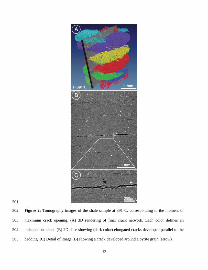
Figure 2: Tomography images of the shale sample at 391⁰C, corresponding to the moment of 502

maximum crack opening. (A) 3D rendering of final crack network. Each color defines an 503

independent crack. (B) 2D slice showing (dark color) elongated cracks developed parallel to the 504

bedding. (C) Detail of image (B) showing a crack developed around a pyrite grain (arrow). 505

24

506

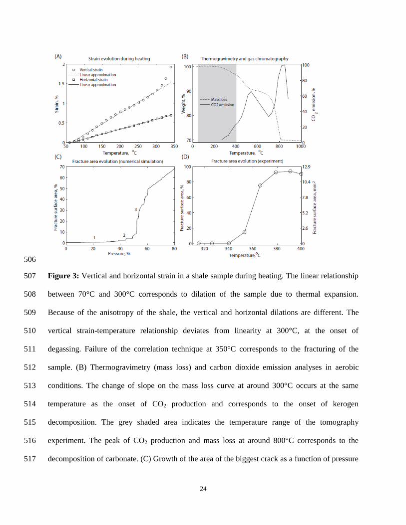
Figure 3: Vertical and horizontal strain in a shale sample during heating. The linear relationship 507

between 70°C and 300°C corresponds to dilation of the sample due to thermal expansion. 508

Because of the anisotropy of the shale, the vertical and horizontal dilations are different. The 509

vertical strain-temperature relationship deviates from linearity at 300°C, at the onset of 510

degassing. Failure of the correlation technique at 350°C corresponds to the fracturing of the 511

sample. (B) Thermogravimetry (mass loss) and carbon dioxide emission analyses in aerobic 512

conditions. The change of slope on the mass loss curve at around 300°C occurs at the same 513

temperature as the onset of CO2 production and corresponds to the onset of kerogen 514

decomposition. The grey shaded area indicates the temperature range of the tomography 515

experiment. The peak of CO2 production and mass loss at around 800°C corresponds to the 516

decomposition of carbonate. (C) Growth of the area of the biggest crack as a function of pressure 517

25

(% of maximum applied pressure) in the 2D lattice model. (1-3) – three stages of crack evolution 518

corresponding to nucleation, growth and coalescence (see corresponding snapshots 1-3B in 519

Figure 5). (D) Fracture evolution in the experiment. Growth of the surface area of the largest 520

crack (in % of the sample cross-sectional area and in mm²) as a function of temperature. The 521

slight decrease of fracture surface area observed after 390⁰C is attributed to partial crack closing 522

after fluid expulsion. 523

524

525

526

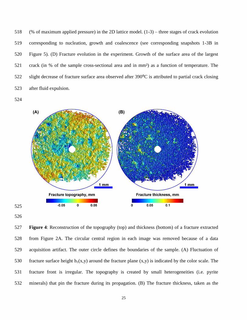
Figure 4: Reconstruction of the topography (top) and thickness (bottom) of a fracture extracted 527

from Figure 2A. The circular central region in each image was removed because of a data 528

acquisition artifact. The outer circle defines the boundaries of the sample. (A) Fluctuation of 529

fracture surface height h1(x,y) around the fracture plane (x,y) is indicated by the color scale. The 530

fracture front is irregular. The topography is created by small heterogeneities (i.e. pyrite 531

minerals) that pin the fracture during its propagation. (B) The fracture thickness, taken as the 532

26

difference between the upper surface h1(x,y) and lower surface h2(x,y) of the fracture, is 533

indicated by the color scale. The thickness is quasi-constant and it is perturbed by pyrite 534

inclusions. 535

536

537 Figure 5: Comparison of crack evolution in the experiment and numerical model. (A) Crack 538

propagation dynamics during heating in the experiment. View of the cracks in a kerogen rich 539

layer viewed from a direction perpendicular to the average plane of the cracks. (1) Numerous 540

small cracks nucleated at ~350⁰C. Each crack is indicated by a different color. (2) Cracks grew 541

and merged with increasing temperature. (3) Ultimately all cracks merged into a single sample-542

wide crack. The circular central region in each image was removed because of a data acquisition 543

artifact. (B) 2D lattice model at three stages of crack development: nucleation (1), growth (2) and 544

coalescence (3) of cracks (see three stages of the area growth (1-3) in Figure 3C). 545

27

546

Figure 6: The correlation between vertical strain evolution (perpendicular to the shale 547

lamination) during heating, mass loss, CO2 emission and growth of fracture area in the shale 548

sample. The onset of the mass loss and CO2 emission corresponds to decomposition of organic 549

material. The nonlinear strain growth in the vertical direction, which is caused by internal fluid 550

pressure buildup, leads to the fracturing at 340⁰C. 551

552

28

553

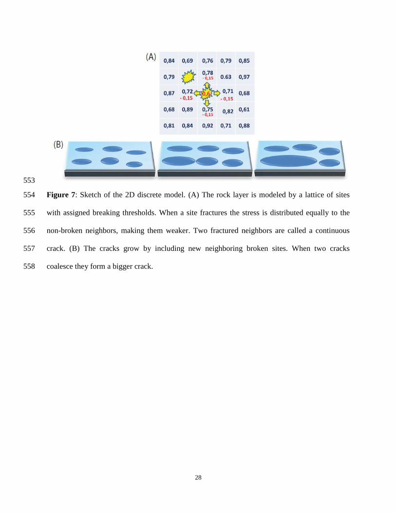
Figure 7: Sketch of the 2D discrete model. (A) The rock layer is modeled by a lattice of sites 554

with assigned breaking thresholds. When a site fractures the stress is distributed equally to the 555

non-broken neighbors, making them weaker. Two fractured neighbors are called a continuous 556

crack. (B) The cracks grow by including new neighboring broken sites. When two cracks 557

coalesce they form a bigger crack. 558