5-4 Electrostatic Boundary Value Problems - KU · PDF fileboundary conditions to find a unique...

11/8/2004 Section 5_4 Electrostatic Boundary Value Problems blank 1/2

Jim Stiles The Univ. of Kansas Dept. of EECS

5-4 Electrostatic Boundary Value Problems

Reading Assignment: pp. 149-157 Q: A: We must solve differential equations, and apply boundary conditions to find a unique solution. In EE and CoE, we typically use a voltage source to apply boundary conditions on electric potential function ( )V r . This process is best demonstrated with a series of examples: Example: Dielectric Filled Parallel Plates

11/8/2004 Section 5_4 Electrostatic Boundary Value Problems blank 2/2


Example: Charge Filled Parallel Plates Example: The Electrostatic Fields of a Coaxial Line

11/8/2004 Example Dielectric Filled Parallel Plates 1/8


Example: Dielectric Filled Parallel Plates

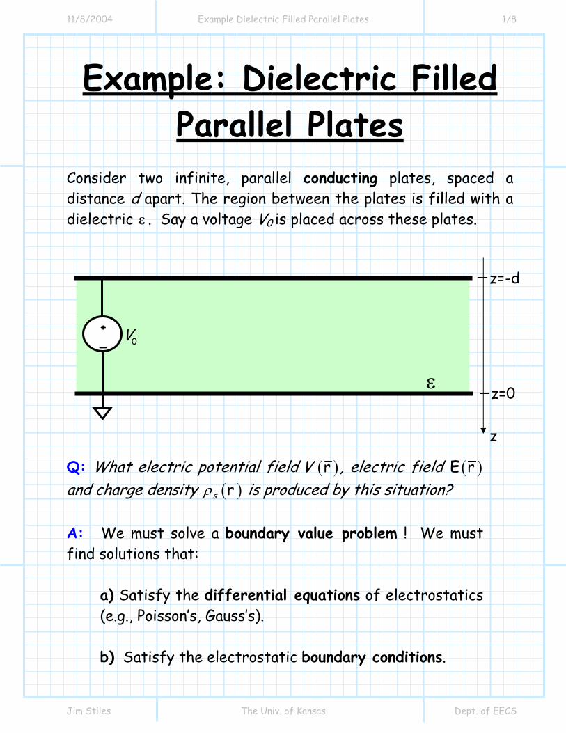
Consider two infinite, parallel conducting plates, spaced a distance d apart. The region between the plates is filled with a dielectric ε . Say a voltage V0 is placed across these plates. Q: What electric potential field ( )rV , electric field ( )rE and charge density ( )rsρ is produced by this situation? A: We must solve a boundary value problem ! We must find solutions that:

a) Satisfy the differential equations of electrostatics (e.g., Poisson’s, Gauss’s). b) Satisfy the electrostatic boundary conditions.

ε

+ _ 0V

z

z=0

z=-d



Q: Yikes! Where do we even start ? A: We might start with the electric potential field ( )rV , since it is a scalar field.

a) The electric potential function must satisfy Poisson’s equation:

( ) ( )2 rr vV ρ−∇ =

ε

b) It must also satisfy the boundary conditions:

( ) ( )0 0 0 V z d V V z= − = = =

Consider first the dielectric region ( 0d z− < < ). Since the region is a dielectric, there is no free charge, and:

( )r 0vρ =

Therefore, Poisson’s equation reduces to Laplace’s equation:

( )2 r 0V∇ =

This problem is greatly simplified, as it is evident that the solution ( )rV is independent of coordinates and yx . In other words, the electric potential field will be a function of coordinate z only:

( ) ( )rV V z=



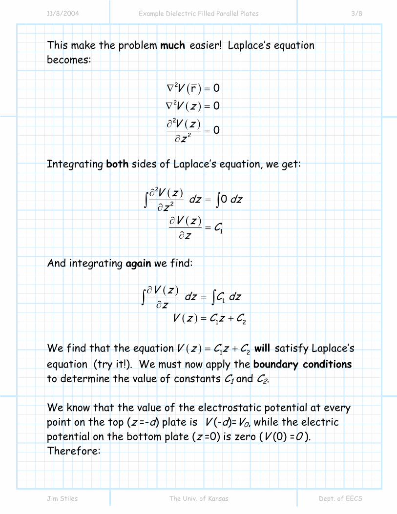
This make the problem much easier! Laplace’s equation becomes:

( )( )

( )

2

2

2

2

r 00

0

VV zV z

z

∇ =

∇ =

∂=

∂

Integrating both sides of Laplace’s equation, we get:

( )

( )

2

2

1

0V z dz dzz

V z Cz

∂=

∂∂

=∂

∫ ∫

And integrating again we find:

( )

( )

1

1 2

V z dz C dzz

V z C z C

∂=

∂= +

∫ ∫

We find that the equation ( ) 1 2V z C z C= + will satisfy Laplace’s equation (try it!). We must now apply the boundary conditions to determine the value of constants C1 and C2. We know that the value of the electrostatic potential at every point on the top (z =-d) plate is V (-d)=V0, while the electric potential on the bottom plate (z =0) is zero (V (0) =0 ). Therefore:



( )

( ) ( )

1 2 0

1 20 0 0

V z d C d C V

V z C C

= − = − + =

= = + =

Two equations and two unknowns (C1 and C2)! Solving for C1 and C2 we get:

02 10 and VC C

d= = −

and therefore, the electric potential field within the dielectric is found to be:

( ) ( )0r 0V zV d zd−

= − ≤ ≤

Before we proceed, let’s do a sanity check! In other words, let’s evaluate our answer at z = 0 and z = -d, to make sure our result is correct:

( ) ( )00

V dV z d Vd

− −= − = =

and

( ) ( )0 00 0

VV zd

−= = =



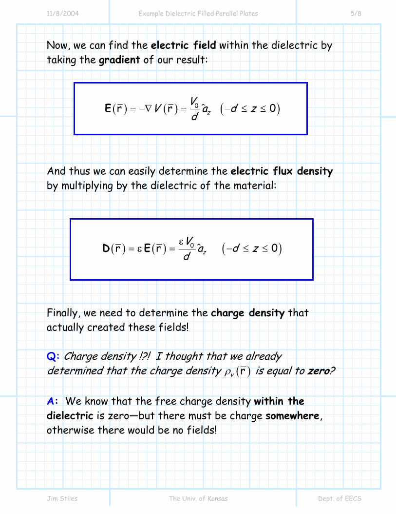
Now, we can find the electric field within the dielectric by taking the gradient of our result:

( ) ( ) ( )0r r 0zVV a d zd

= −∇ = − ≤ ≤E ˆ

And thus we can easily determine the electric flux density by multiplying by the dielectric of the material:

( ) ( ) ( )0r r 0zV a d zd

= = − ≤ ≤D E ˆε

ε

Finally, we need to determine the charge density that actually created these fields! Q: Charge density !?! I thought that we already determined that the charge density ( )rvρ is equal to zero? A: We know that the free charge density within the dielectric is zero—but there must be charge somewhere, otherwise there would be no fields!



Recall that we found that at a conductor/dielectric interface, the surface charge density on the conductor is related to the electric flux density in the dielectric as:

( ) ( )r rˆn n sD a ρ= ⋅ =D

First, we find that the electric flux density on the bottom surface of the top conductor (i.e., at z d= − ) is:

( ) 0 0r z zz dz d

V Va ad d=−

=−

= =D ˆ ˆε ε

For every point on bottom surface of the top conductor, we find that the unit vector normal to the conductor is:

ˆ ˆn za a= Therefore, we find that the surface charge density on the bottom surface of the top conductor is:

( ) ( )

( )

0

0

r r

s n

z z

z da

Va ad

V z dd

ρ + =−= ⋅

= ⋅

= = −

Dˆ

ˆ ˆε

ε



Likewise, we find the unit vector normal to the top surface of the bottom conductor is (do you see why):

ˆ ˆn za a= −

Therefore, evaluating the electric flux density on the top surface of the bottom conductor (i.e., 0z = ), we find:

( ) ( )

( )

0

0

0

r r

0

s n z

z z

a

Va ad

V zd

ρ − == ⋅

= − ⋅

= =

Dˆ

ˆ ˆε

−ε

We should note several things about these solutions: 1) ( )x r 0∇ =E 2) ( ) ( )2r 0 and r 0V∇ ⋅ = ∇ =D 3) ( ) ( )r and rD E are normal to the surface of the conductor (i.e., their tangential components are equal to zero). 4) The electric field is precisely the same as that given by using superposition and eq. 4.20 in section 4-5!



I.E.:

( ) ( )0r 0ˆ ˆ ˆs sz z z

Va a a d zd

ρ ρ+ −= − = − < <E2ε 2ε

In other words, the fields ( ) ( ) ( )r , r , and rVE D are attributable to charge densities ( ) ( )r and r s sρ ρ+ − .

ε

+ _ 0V

z

z=0

z=-d

_ _ _ _ _ _ _ _ _ _ _ _ _ _ _ _ _ _ _ _ _ _ _ _ _ _ _ _

+ + + + + + + + + + + + + + + + + + + + + + + + + + + + + + + + + +

( )rE

( )rsρ +

( )rsρ −

11/8/2004 Example Charge Filled Parallel Plates 1/4


Example: Charge Filled Parallel Plates

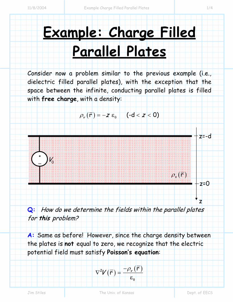
Consider now a problem similar to the previous example (i.e., dielectric filled parallel plates), with the exception that the space between the infinite, conducting parallel plates is filled with free charge, with a density:

( )r (-d 0)v z zρ = − < <0ε

Q: How do we determine the fields within the parallel plates for this problem? A: Same as before! However, since the charge density between the plates is not equal to zero, we recognize that the electric potential field must satisfy Poisson’s equation:

( ) ( )2 rr vV ρ−∇ =

0ε

( )v rρ

+ _ 0V

z

z=0

z=-d



For the specific charge density ( )rv zρ = − 0ε :

( ) ( )2 rr vV zρ−∇ = =

0ε

Since both the charge density and the plate geometry are independent of coordinates x and y, we know the electric potential field will be a function of coordinate z only (i.e., ( ) ( )rV V z= ).

Therefore, Poisson’s equation becomes:

( ) ( )22

2

zz

VV zz

∂∇ = =

∂

We can solve this differential equation by first integrating both sides:

( )

( )

2

2

2

1

z

z2

V dz z dzz

V z Cz

∂=

∂∂

= +∂

∫ ∫

And then integrating a second time:

( )

( )

2

1

3

1 2

r2

r6

V zdz C dzz

zV C z C

∂ ⎛ ⎞= +⎜ ⎟∂ ⎝ ⎠

= + +

∫ ∫



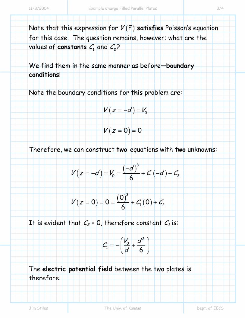
Note that this expression for ( )rV satisfies Poisson’s equation for this case. The question remains, however: what are the values of constants 1 2 and C C ? We find them in the same manner as before—boundary conditions! Note the boundary conditions for this problem are:

( )

( )

0

0 0

V z d V

V z

= − =

= =

Therefore, we can construct two equations with two unknowns:

( ) ( ) ( )

( ) ( ) ( )

3

0 1 2

3

1 2

6

00 0 0

6

dV z d V C d C

V z C C

−= − = = + − +

= = = + +

It is evident that C2 = 0, therefore constant C1 is:

20

1 6V dCd

⎛ ⎞= − +⎜ ⎟

⎝ ⎠

The electric potential field between the two plates is therefore:



( ) ( )3 2

0r 06 6

Vz dV z d zd

⎛ ⎞= − + − < <⎜ ⎟

⎝ ⎠

Performing our sanity check, we find:

( ) ( ) ( )3 2

0

3 3

0

0

dz -d -d

6 6d6 6

V dVd

dV

V

− ⎛ ⎞= = − +⎜ ⎟

⎝ ⎠−

= + +

=

and

( ) ( ) ( )3 2

00z 0 0

6 60 0 00

V dVd

⎛ ⎞= = − +⎜ ⎟

⎝ ⎠= + +

=

From this result, we can determine the electric field ( )rE , the electric flux density ( )rD , and the surface charge density

( )rsρ , as before. Note, however, that the permittivity of the material between the plates is 0ε , as the “dielectric” between the plates is free-space.

11/8/2004 Example The Electorostatic Fields of a Coaxial Line 1/10


Example: The Electrostatic Fields of a Coaxial Line

A common form of a transmission line is the coaxial cable. The coax has an outer diameter b, and an inner diameter a. The space between the conductors is filled with dielectric material of permittivity ε . Say a voltage V0 is placed across the conductors, such that the electric potential of the outer conductor is zero, and the electric potential of the inner conductor is V0.

ε

b

a

+ V0 -

Coax Cross-Section

Outer Conductor

Inner Conductor



The potential difference between the inner and outer conductor is therefore V0 – 0 = V0 volts. Q: What electric potential field ( )rV , electric field ( )rE and charge density ( )rsρ is produced by this situation? A: We must solve a boundary-value problem! We must find solutions that:

a) Satisfy the differential equations of electrostatics (e.g., Poisson’s, Gauss’s). b) Satisfy the electrostatic boundary conditions.

Yikes! Where do we start ? We might start with the electric potential field ( )rV , since it is a scalar field.

a) The electric potential function must satisfy Poisson’s equation:

( ) ( )2 rr vV ρ−∇ =

ε

b) It must also satisfy the boundary conditions:

( ) ( )0 0 V a V V bρ ρ= = = =



Consider first the dielectric region (a bρ< < ). Since the region is a dielectric, there is no free charge, and:

( )r 0vρ =

Therefore, Poisson’s equation reduces to Laplace’s equation:

( )2 r 0V∇ =

This particular problem (i.e., coaxial line) is directly solvable because the structure is cylindrically symmetric. Rotating the coax around the z-axis (i.e., in the aφ direction) does not change the geometry at all. As a result, we know that the electric potential field is a function of ρ only ! I.E.,:

( ) ( )rV V ρ=

This make the problem much easier. Laplace’s equation becomes:

( )( )

( )

( )

2

2

r 00

1 0 0 0

0

VV

V

V

ρ

ρρ

ρ ρ ρ

ρρ

ρ ρ

∇ =

∇ =

∂⎛ ⎞∂+ + =⎜ ⎟∂ ∂⎝ ⎠∂⎛ ⎞∂

=⎜ ⎟∂ ∂⎝ ⎠

Be very careful during this step! Make sure you implement the gul durn Laplacian operator correctly.



Integrating both sides of the resulting equation, we find:

( )

( )1

0V d d

V C

ρρ ρ ρ

ρ ρρ

ρρ

∂⎛ ⎞∂=⎜ ⎟∂ ∂⎝ ⎠

∂=

∂

∫ ∫

where C1 is some constant. Rearranging the above equation, we find:

( ) 1V Cρρ ρ

∂=

∂

Integrating both sides again, we get:

( )

( ) [ ]

1

1 2ln

V Cd dp

V C C

ρρ ρ

ρ

ρ ρ

∂=

∂

= +

∫ ∫

We find that this final equation ( ( ) [ ]1 2lnV C Cρ ρ= + ) will satisfy Laplace’s equation (try it!). We must now apply the boundary conditions to determine the value of constants C1 and C2.

* We know that on the outer surface of the inner conductor (i.e., aρ = ), the electric potential is equal to V0 (i.e., ( ) 0V a Vρ = = ).



* And, we know that on the inner surface of the outer conductor (i.e., bρ = ) the electric potential is equal to zero (i.e., ( ) 0V bρ = = ).

Therefore, we can write:

( ) [ ]

( ) [ ]

1 2 0

1 2

ln

ln 0

V a C a C V

V b C b C

ρ

ρ

= = + =

= = + =

Two equations and two unknowns (C1 and C2)! Solving for C1 and C2 we get:

[ ] [ ]

[ ]

0 01

02

ln b ln a ln b/a

ln bln b/a

V VC

VC

− −= =

− ⎡ ⎤⎣ ⎦

=⎡ ⎤⎣ ⎦

and therefore, the electric potential field within the dielectric is found to be:

( ) [ ] [ ] ( )00 ln b lnr ln b/a ln b/a

VVV b aρρ

−= + > >

⎡ ⎤ ⎡ ⎤⎣ ⎦ ⎣ ⎦



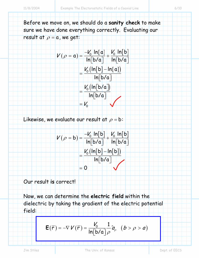
Before we move on, we should do a sanity check to make sure we have done everything correctly. Evaluating our result at aρ = , we get:

( ) [ ] [ ]

[ ] [ ]( )

( )

00

0

0

0

ln b ln aa ln b/a ln b/a

ln b ln aln b/a

ln b/aln b/a

VVV

V

V

V

ρ−

= = +⎡ ⎤ ⎡ ⎤⎣ ⎦ ⎣ ⎦

−=

⎡ ⎤⎣ ⎦

⎡ ⎤⎣ ⎦=⎡ ⎤⎣ ⎦

=

Likewise, we evaluate our result at bρ = :

( ) [ ] [ ]

[ ] [ ]( )

0 0

0

ln b ln bb

ln b/a ln b/a

ln b ln bln b/a

0

V VV

V

ρ−

= = +⎡ ⎤ ⎡ ⎤⎣ ⎦ ⎣ ⎦

−=

⎡ ⎤⎣ ⎦=

Our result is correct! Now, we can determine the electric field within the dielectric by taking the gradient of the electric potential field:

( ) ( ) ( )0 1r r ln b/a

VV a b aρ ρρ

= −∇ = > >⎡ ⎤⎣ ⎦

E ˆ



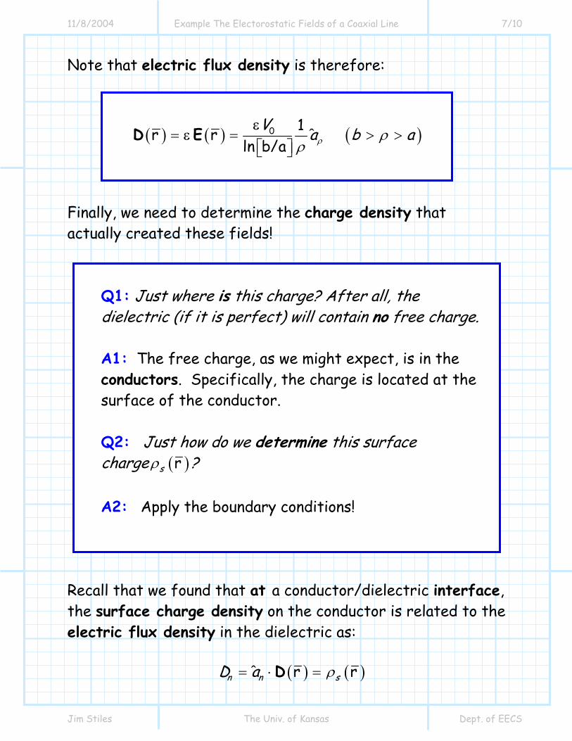
Note that electric flux density is therefore:

( ) ( ) ( )0 1r r ln b/a

ˆV a b aρ ρ

ρ= = > >

⎡ ⎤⎣ ⎦D E ε

ε

Finally, we need to determine the charge density that actually created these fields!

Q1: Just where is this charge? After all, the dielectric (if it is perfect) will contain no free charge. A1: The free charge, as we might expect, is in the conductors. Specifically, the charge is located at the surface of the conductor. Q2: Just how do we determine this surface charge ( )rsρ ? A2: Apply the boundary conditions!

Recall that we found that at a conductor/dielectric interface, the surface charge density on the conductor is related to the electric flux density in the dielectric as:

( ) ( )r rˆn n sD a ρ= ⋅ =D



First, we find that the electric flux density on the surface of the inner conductor (i.e., at aρ = ) is:

( ) 0a

0

1rln b/a

1ln b/a

a

Va

Vaa

ρρρ

ρ

ρ==

=⎡ ⎤⎣ ⎦

=⎡ ⎤⎣ ⎦

D ˆ

ˆ

ε

ε

For every point on outer surface of the inner conductor, we find that the unit vector normal to the conductor is:

n aa ρ=ˆ ˆ Therefore, we find that the surface charge density on the outer surface of the inner conductor is:

( ) ( )

( )

a

0

0

r r

1ln b/a

1 aln b/a

sa naVa a

aV

a

ρ

ρ ρ

ρ

ρ

== ⋅

= ⋅⎡ ⎤⎣ ⎦

= =⎡ ⎤⎣ ⎦

Dˆ

ˆ ˆε

ε



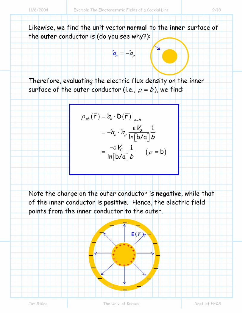
Likewise, we find the unit vector normal to the inner surface of the outer conductor is (do you see why?):

n aa ρ= −ˆ ˆ

Therefore, evaluating the electric flux density on the inner surface of the outer conductor (i.e., bρ = ), we find:

( ) ( )

( )

0

0

r r

1ln b/a

1 bln b/a

nsb ba

Va ab

Vb

ρ

ρ ρ

ρ

ρ

== ⋅

= − ⋅⎡ ⎤⎣ ⎦

= =⎡ ⎤⎣ ⎦

Dˆ

ˆ ˆε

−ε

Note the charge on the outer conductor is negative, while that of the inner conductor is positive. Hence, the electric field points from the inner conductor to the outer.

( )rE

+ + + + + + + + + + + +

+ + +

+

_

_

_ _

_

_

_

_

_

_

_ _

_

_

_

_



We should note several things about these solutions:

1) ( )x r 0∇ =E 2) ( ) ( )2r 0 and r 0V∇ ⋅ = ∇ =D 3) ( ) ( )r and rD E are normal to the surface of the conductor (i.e., their tangential components are equal to zero). 4) The electric field is precisely the same as that given by eq. 4.31 in section 4-5!

( ) ( )0 1r ln b/a

ˆ ˆsa Va a a b aρ ρρ ρρ ρ

= = > >⎡ ⎤⎣ ⎦

Eε

In other words, the fields ( ) ( ) ( )r , r , and rVE D are attributable to free charge densities ( ) ( )r and rsa sbρ ρ .

Date post:	06-Mar-2018
Category:	Documents
Upload:	hakien
View:	221 times
Download:	1 times

5-4 Electrostatic Boundary Value Problems - KU · PDF fileboundary conditions to find a unique...

Documents