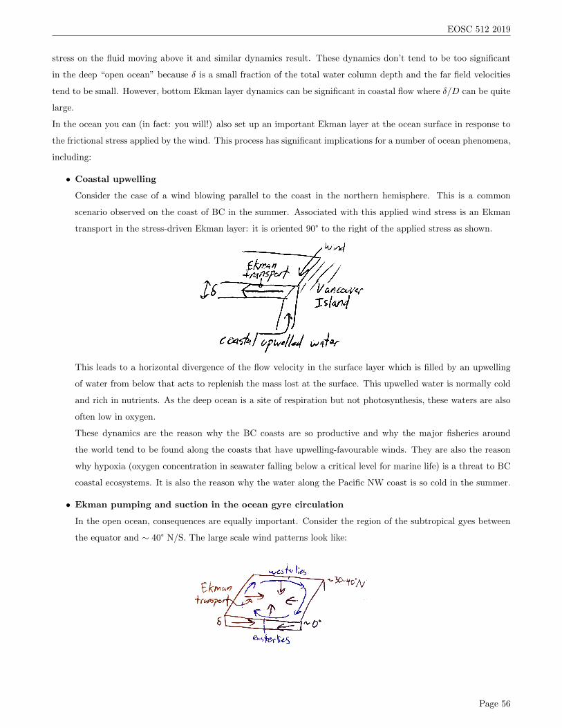
EOSC 512 2019 5 Boundary Conditions and Frictional Boundary Layers The boundary conditions to apply to these equations of motion are just as important as the equations themselves! It is important to keep in mind that the formulation of a problem in fluid mechanics requires the specification of the pertinent equations and the relevant boundary conditions with equal care and attention. In GFD in particular, there are many examples of important physical problems, like the physics of surface waves on water, in which the fundamental dynamics are contained entirely within the boundary conditions. Likewise, the theory for cyclogensis (spontaneous appearance of weather waves in the atmosphere) is similar. In these problems, the boundary conditions are dynamical in nature and their correct formulation is critical to understanding the relevant physical phenomena. 5.1 Boundary conditions at a solid surface The most straightfoward conditions apply when the fluid is in contact with a solid surface. For the following arguments, consider a solid surface described by the equation S(~ x, t) = 0. It has a normal vector ˆ n that is oriented in the direction of the gradient of S, rS. Note that this implies: ˆ n = rS |rS| = rS @S @n (5.1) Where n is the distance coordinate normal to the surface. 1. Condition on the normal velocity of a fluid element on the surface: If the surface is solid, we must impose the condition that there is no fluid flow through the surface. Additionally, if the surface is moving, this implies that the velocity of the fluid normal to the surface must equal the velocity of the surface normal itself. If fluid cannot go through the surface, a condition of no normal-flow must be imposed. This implies: DS Dt =0 on S =0 @ S @ t + ~ u · rS =0 substituting ˆ n as above, @ S @ t + ~ u · @ S @ n ˆ n =0 ~ u · ˆ n = - @S @t @S @n = @ n @ t S ⌘ u n (5.2) Page 44
Transcript
EOSC 512 2019
5 Boundary Conditions and Frictional Boundary Layers
The boundary conditions to apply to these equations of motion are just as important as the equations themselves!
It is important to keep in mind that the formulation of a problem in fluid mechanics requires the specification of
the pertinent equations and the relevant boundary conditions with equal care and attention.
In GFD in particular, there are many examples of important physical problems, like the physics of surface waves
on water, in which the fundamental dynamics are contained entirely within the boundary conditions. Likewise, the
theory for cyclogensis (spontaneous appearance of weather waves in the atmosphere) is similar.
In these problems, the boundary conditions are dynamical in nature and their correct formulation is critical to
understanding the relevant physical phenomena.
5.1 Boundary conditions at a solid surface
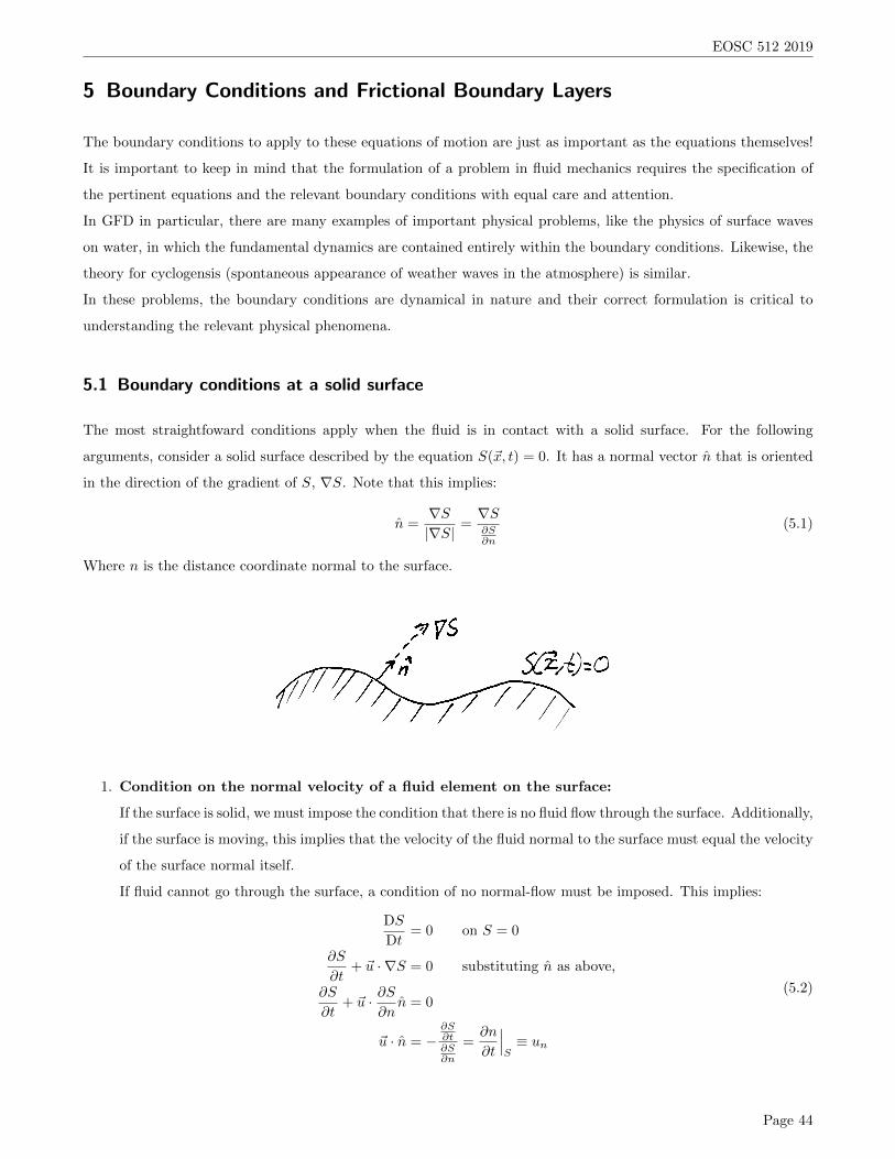
The most straightfoward conditions apply when the fluid is in contact with a solid surface. For the following
arguments, consider a solid surface described by the equation S(~x, t) = 0. It has a normal vector n that is oriented
in the direction of the gradient of S, rS. Note that this implies:
n =rS
|rS|=
rS
@S
@n
(5.1)
Where n is the distance coordinate normal to the surface.
1. Condition on the normal velocity of a fluid element on the surface:
If the surface is solid, we must impose the condition that there is no fluid flow through the surface. Additionally,
if the surface is moving, this implies that the velocity of the fluid normal to the surface must equal the velocity
of the surface normal itself.
If fluid cannot go through the surface, a condition of no normal-flow must be imposed. This implies:
DS
Dt= 0 on S = 0
@S
@t+ ~u ·rS = 0 substituting n as above,
@S
@t+ ~u ·
@S
@nn = 0
~u · n = �
@S
@t
@S
@n
=@n
@t
���S
⌘ un
(5.2)
Page 44
EOSC 512 2019
Where un is the velocity of the surface normal. Of course, if the surface is not moving, un = 0. This condition
is called the kinematic boundary condition.
2. Condition on the tangential velocity of a fluid element on the surface:
In the presence of friction (whenever µ 6= 0), we observe that the fluid at the boundary sticks to the boundary.
This is often called the “no-slip” boundary condition. In this case, the tangential velocity of the fluid is also
equal to the tangential velocity of the boundary.
The microscopic explanation (easily verified for a gas) is that as a gas molecule strikes the surface, it is captured
by the surface potential of the molecules constituting the boundary. The gas molecules are captured long
enough to have their average motion annulled and their eventual escape velocity is random (no macroscopic
mean velocity is imparted by this process)
Except for very rare gases with extremely low density (for which this randomization of the escape velocity –
called thermalization – may be incomplete) the appropriate boundary condition is:
~u · t = ut (5.3)
Where ut is the tangential velocity of the surface.
It is important to note that this expression is independent of the magnitude of the viscosity coe�cient even
though the condition is physically due to the presence of frictional stresses in the fluid.
One might imagine that for small enough values of µ, the viscous terms in the Navier-Stokes equations could
be ignored. However, eliminating the viscous terms lowers the order of the di↵erential equations
so that they are no longer able to satisfy all boundary conditions! This is one of the factors that
puzzled those studying fluid mechanics in its enfancy. The resolution of this apparent paradox forms an
important part of the dynamics which we shall explore in future examples.
5.2 Boundary conditions at a fluid interface
The boundary conditions at the interface of two immiscible fluids is more interesting – and highly relevant to the
boundary condition between the ocean and the atmosphere.
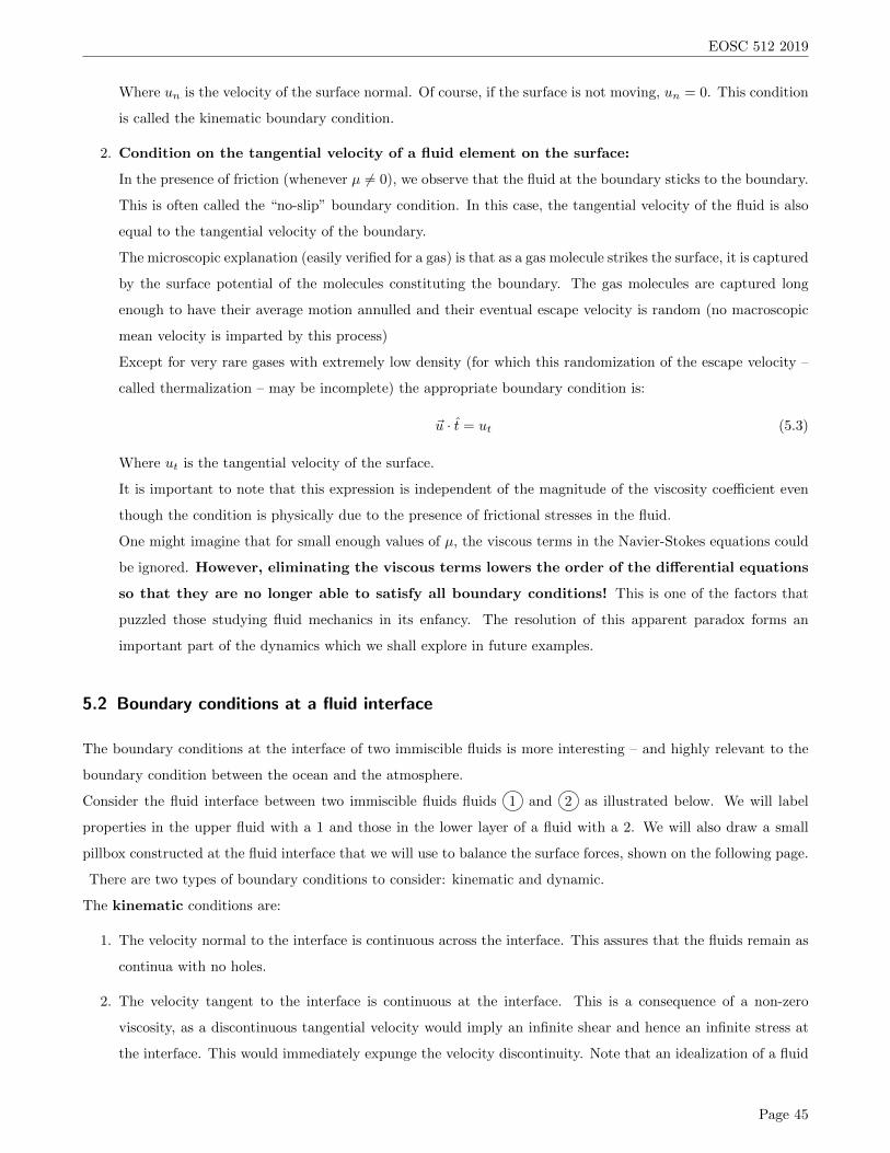
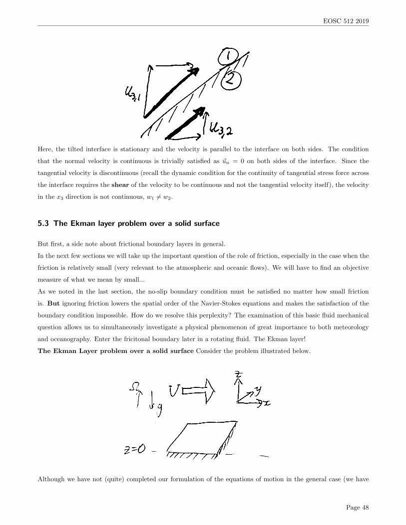
Consider the fluid interface between two immiscible fluids fluids 1 and 2 as illustrated below. We will label
properties in the upper fluid with a 1 and those in the lower layer of a fluid with a 2. We will also draw a small
pillbox constructed at the fluid interface that we will use to balance the surface forces, shown on the following page.
There are two types of boundary conditions to consider: kinematic and dynamic.
The kinematic conditions are:
1. The velocity normal to the interface is continuous across the interface. This assures that the fluids remain as
continua with no holes.
2. The velocity tangent to the interface is continuous at the interface. This is a consequence of a non-zero
viscosity, as a discontinuous tangential velocity would imply an infinite shear and hence an infinite stress at
the interface. This would immediately expunge the velocity discontinuity. Note that an idealization of a fluid
Page 45
EOSC 512 2019
that completely ignores viscosity can allow such discontinuities and again the relationship between a fluid
with a small viscosity and one with µ = 0 is a singular one that needs special examination.
Dynamic conditions:
Consider the small pillbox constructed at the fluid interface shown in the previous figure. If we balance the forces
on the mass in the box and then take the limit dh ! 0, the volume forces will go to zero faster than the surface
forces. As in our argument for the symmetry of the stress tensor, we can argue that in this limit, the surfaces forces
must balance – except for the action of surface tension forces.
~⌃1(n1) + ~⌃2(n2) = ��
✓1
Ra
+1
Rb
◆n (5.4)
Where Ra and Rb are the radii of curvature of the surface in any two orthogonal directions and � is the surface
tension coe�cient. Noting that n1 = �n2 ⌘ n and ~⌃2(�n) = �~⌃2(n) by Newton’s third law, this expression
becomes:
~⌃1(�n)� ~⌃2(�n) = ��
✓1
Ra
+1
Rb
◆n (5.5)
In terms of the stress tensor (recalling ⌃i(n) = �ij nj):
�1,ij nj � �2,ij nj + �
✓1
Ra
+1
Rb
◆ni = 0 (5.6)
Consider first the dynamic conditions for the continuity of normal stress force across the interface:
The stress in the direction normal to the surface is then (Recalling that this is given by ⌃i(n) · n):
�1,ij ninj � �2,ij ninj + �
✓1
Ra
+1
Rb
◆= 0 (5.7)
Using our expression for the stress tensor in terms of the contributions arising from the symmetric and antisymmetric
parts of the deformation tensor (Recall �ij = �P �ij + 2µeij + �ekk�ij) and noting that nini = 1: