115 CLIMATE RECONSTRUCTIONS DERIVED FROM GLOBAL GLACIER LENGTH RECORDS INCLUDING A CASE-STUDY FOR EUROPEAN GLACIERS * Abstract – Glaciers have fluctuated in historic times and the length fluctuations of many glaciers are known. From these glacier length records, a climate reconstruction described in terms of a reconstruction of the equilibrium line altitude (ELA) or the mass balance can be extracted. In order to derive a climate signal from numerous glacier length records, a model is needed that takes into account the main characteristics of a glacier, but uses little information about the glacier itself. Therefore, a simple analytical model was developed based on the assumption that the change in glacier length can be described by a linear response equation. The model takes into account the geometry of the glacier, the length response time and the mass balance - surface elevation feedback. The model was tested on seventeen European glacier length records. The results revealed that the ELA of these glaciers increased on average 54 m between 1920 and 1950. The results were compared to mass balance reconstructions calculated with a numerical flowline model and derived from historical temperature and precipitation records. The findings indicate that the analytical model is useful to gain information about historical mass balance rates and ELAs. Then, we derived historic fluctuations in the ELA on the basis of nineteen glacier length records from different parts of the world. The results show that all glaciers of this global data set experienced an increase in the ELA between 1900 and 1960. Between 1910 and 1959, the average increase was 33±8 m. This implies that during the first half of the twentieth century, the climate was warmer or drier than before. The ELAs decreased to lower elevations after around 1960 up to 1980, when most of our ELA reconstructions end. These results can be translated into a global temperature increase of 0.8±0.2 K and a sea level rise of 0.3 mm a –1 for the period 1910–1959. * Based on: Klok, E.J. and Oerlemans, J. 2003. Deriving historical equilibrium-line altitudes from a glacier length record by linear inverse modelling. The Holocene , 13 (3), 343-351; and Klok, E.J. and Oerlemans, J. 2003. Climate reconstructions derived from global glacier length records. Arctic, Antarctic and Alpine Research , submitted. 5
Transcript
115
CLIMATE RECONSTRUCTIONS DERIVED FROM
GLOBAL GLACIER LENGTH RECORDS
INCLUDING A CASE-STUDY FOR EUROPEAN
GLACIERS*
Abstract – Glaciers have fluctuated in historic times and the lengthfluctuations of many glaciers are known. From these glacier lengthrecords, a climate reconstruction described in terms of areconstruction of the equilibrium line alti tude (ELA) or the massbalance can be extracted. In order to derive a climate signal fromnumerous glacier length records, a model is needed that takes intoaccount the main characteristics of a glacier, but uses littleinformation about the glacier i tself. Therefore, a simple analyticalmodel was developed based on the assumption that the change inglacier length can be described by a linear response equation. Themodel takes into account the geometry of the glacier, the lengthresponse time and the mass balance - surface elevation feedback.The model was tested on seventeen European glacier lengthrecords. The results revealed that the ELA of these glaciersincreased on average 54 m between 1920 and 1950. The resultswere compared to mass balance reconstructions calculated with anumerical flowline model and derived from historical temperatureand precipitation records. The findings indicate that the analyticalmodel is useful to gain information about historical mass balancerates and ELAs. Then, we derived historic fluctuations in the ELAon the basis of nineteen glacier length records from different partsof the world. The results show that all glaciers of this global dataset experienced an increase in the ELA between 1900 and 1960.Between 1910 and 1959, the average increase was 33±8 m. Thisimplies that during the first half of the twentieth century, theclimate was warmer or drier than before. The ELAs decreased tolower elevations after around 1960 up to 1980, when most of ourELA reconstructions end. These results can be translated into aglobal temperature increase of 0.8±0.2 K and a sea level rise of 0.3mm a–1 for the period 1910–1959.
* Based on: Klok, E.J. and Oerlemans, J. 2003. Deriving historical equilibrium-linealtitudes from a glacier length record by linear inverse modelling. The Holocene,13(3), 343-351; and Klok, E.J. and Oerlemans, J. 2003. Climate reconstructionsderived from global glacier length records. Arctic, Antarctic and Alpine Research ,submitted.
5
116
5.1 INTRODUCTION
Glacier length records contain information on how climate haschanged. This information often complements historical meteorologicaldata, as glacier length records generally extend further back in time.Besides, glacier records are often from remote areas and higher altitudes,for which meteorological data are scarce (IPCC, 2001). Hence, glacier lengthrecords form an alternative method for climate reconstruction for periodsand locations for which instrumental or proxy indicators are inadequate orcontradicting. Extracting climatic information from glacier length recordsimplies inverse modelling. Normally, the climate signal extracted fromlength records is represented as a mass-balance history or as areconstruction of the equilibrium line altitude (ELA). ELA reconstructionsresemble transient climate changes more properly than glacier lengthchanges, as the glacier length is subject to the length response time and thesensitivity of a glacier.
Callendar (1950) was probably the first who attempted to extract aclimate signal from the dimensions of a glacier. He presented a relationbetween the height of the firn line and the glacier length, including thewidth at the glacier snout, the glacier width and slope at the firn linealtitude and a constant ratio between the accumulation and ablation area.Other simple methods to reconstruct the ELA are (I) the median elevation ofa glacier (Manley, 1959), which is the elevation midway between the glaciersnout and the base of the headwall, (II) the THAR (Toe-to-HeadwallAltitude Ratio), which is a fraction of the height range of the glacier(Meierding, 1982), and (III) the ratio of the accumulation area to the total area(AAR) (Porter, 1975). Benn and Lehmkuhl (2000) discussed the applicability ofthese and other commonly used methods for different glacier types. Haeberli
and Hoelzle (1995) developed a simple parameterisation scheme, build onfour geometric parameters (glacier length and area, minimum andmaximum elevation). They reconstructed changes in the mass balance ofglaciers in the European Alps.
However, none of the methods above considers the response time of aglacier. Nye (1965) was the first who used a numerical method to infer themass-balance history of a glacier from its length fluctuations. Oerlemans
(1997), Wallinga and Van de Wal (1998) and Mackintosh and Dugmore (2000) useda numerical flowline model and the procedure of dynamic calibration toderive a mass-balance history. The advantage of a numerical flowline modelis that the geometry, the climate sensitivity and the response time of eachparticular glacier are taken into account. However, numerical flowlinemodels need lots of information, which is not always available. Therefore,they cannot be applied to a large number of glacier records.
117
5 C
LIM
AT
E R
EC
ON
ST
RU
CT
ION
S
DE
RIV
ED
F
RO
M G
LO
BA
L G
LA
CIE
R L
EN
GT
H
RE
CO
RD
S
1600 1700 1800 1900 2000Year
U. Grindelwaldgl., SwitzerlandGlacier d'Argentière, France
Bas Glacier d'Arolla, SwitzerlandMer de Glace, France
Rhonegletscher, Switzeland
Griesgletscher, SwitzerlandVadret da Roseg, SwitzerlandOedenwinkelkees, AustriaLangtalerferner, Austria
Gurglerferner, AustriaPasterzenkees, Austria
Hintereisferner, AustriaForni, Italy
Engabreen, Norway
Nigardsbreen, Norway
Sólheimajökull, Iceland
Svinafellsjökull, Iceland
Gla
cie
r le
ng
th (
un
it is
1 k
m)
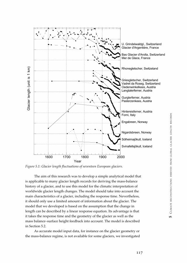
Figure 5.1: Glacier length fluctuations of seventeen European glaciers.
The aim of this research was to develop a simple analytical model thatis applicable to many glacier length records for deriving the mass-balancehistory of a glacier, and to use this model for the climatic interpretation ofworldwide glacier length changes. The model should take into account themain characteristics of a glacier, including the response time. Nevertheless,it should only use a limited amount of information about the glacier. Themodel that we developed is based on the assumption that the change inlength can be described by a linear response equation. Its advantage is thatit takes the response time and the geometry of the glacier as well as themass balance–surface height feedback into account. The model is describedin Section 5.2.
As accurate model input data, for instance on the glacier geometry orthe mass-balance regime, is not available for some glaciers, we investigated
118
the effects of the uncertainties in the input data on the ELA reconstruction.This sensitivity study is presented in Section 5.3.
As a start, we performed a case study and tested the analytical modelfor seventeen European glaciers, the length records of which are shown inFigure 5.1. At the top of the graph, glaciers from the western Alps areshown, followed by glaciers from the eastern Alps, Scandinavia andIceland. These seventeen glaciers, which all retreated between 1850 and1980, were selected because their length records are among the longest of allEuropean glacier records. We calculated reconstructions of the mass balanceand ELA with the analytical model and compared the results with climatereconstructions derived from other methods (Section 5.4).
We then extended this investigation to global glacier length changesand derived historic fluctuations in the equilibrium line altitude (ELA) onthe basis of nineteen glacier length records from different parts of theworld. So far, the climatic interpretation of worldwide glacier lengthfluctuations has been studied occasionally. More frequently, lengthfluctuations of single glaciers or glaciers in one specific region wereinvestigated, e.g. the European Alps (Haeberli and Hoelzle, 1995), the CentralItalian Alps (Pelfini and Smiraglia, 1997), Scandinavia (Bogen et al., 1989), thePatagonian Ice Fields (Warren and Sugden, 1993; Aniya, 1999), the NorthCascade glaciers (Pelto and Hedlund, 2001), Northern Eurasia (Solomina, 2000),Tien Shan (Savoskul, 1997), New Zealand (Chinn, 1996) and the tropics (Kaser,
1999). On the other hand, Oerlemans (1994) compared the retreat of 48glaciers from different regions of the world. He estimated from this a globallinear warming trend of 0.66 K per century, but did not take the responsetime of the glaciers into account. Hoelzle et al. (2003) also investigated 90glaciers worldwide. They estimated –from cumulative glacier lengthchanges– a global mean specific mass balance of –0.25 m w.e. a–1 since 1900.The analytical model that we used for the climatic interpretation of lengthfluctuations is more sophisticated than the models of Oerlemans (1994) andHoelzle et al. (2003), as we corrected for the length response time and treatedthe geometry of each glacier more comprehensively.
In Section 5.5, we describe the nineteen glaciers of our global data set.The ELA and mass-balance reconstructions derived from the length recordsare presented in Section 5.6. The results are also interpreted in terms ofchanges in air temperature (Section 5.6.4). Section 5.7 contains a discussionof the results and Section 5.8 a summary.
119
5 C
LIM
AT
E R
EC
ON
ST
RU
CT
ION
S
DE
RIV
ED
F
RO
M G
LO
BA
L G
LA
CIE
R L
EN
GT
H
RE
CO
RD
S
5.2 THE ANALYTICAL MODEL
5.2.1 LINEAR RESPONSE EQUATION
A glacier responds to a change in the mass balance (and the ELA) bychanging its length. The size of the length change depends on severalfactors, such as the geometry, the slope and the mass-balance profile of theglacier. For relatively small length fluctuations compared to the total glacierlength, it is assumed that the change in glacier length can be described by alinear response equation:
dL t
dt
cE t L t
trL
' ( ) ' ( ) ' ( )= −
+(5.1)
where L’(t) is the glacier length with regard to a reference length (L0) (m), tis time (a), c is the climate sensitivity (–), E’(t) is the ELA with regard to areference altitude (E0) (m) and trL is the length response time of the glacier(a) (see Figure 5.2 for explanation of the symbols). The concept of thisanalytical model was first put forward by Oerlemans (2001).
Figure 5.2: Schematic outline of a glacier, showing some of the parameters of theanalytical model.
The reference length, L0, is calculated as the mean of a glacier lengthrecord. The climate sensitivity (c) is a factor that relates a change in the
120
glacier’s steady-state length to a change in the ELA. For large lengthfluctuations, the analytical model is not valid because the glacier geometrycan change significantly when the glacier retreats or advances over a largedistance. As a result, the response time and the climate sensitivity cannot bekept constant.
The inverse of the linear response equation can be used to calculatethe historic ELAs:
E tcL t
dL
dtrL' ( ) ''
= − +
1(5.2)
If E’(t) is multiplied by the mass-balance gradient at the equilibrium linealtitude (βE), this equation can be used to calculate a mass-balance
reconstruction (B’(t)). Methods to estimate the length response time and theclimate sensitivity are given in Section 5.2.2. First, how the time derivativeof a length record can be calculated is described.
Generally, glacier length records are not smooth records (see Figure5.1). Linear interpolation between the observed data points is applied,assuming that the glaciers have not fluctuated substantially during theperiods between these points. It is likely that they were not larger duringthe period in between the data points, otherwise moraines would have beendeposited. However, glaciers could have been smaller during these periods.Taking the time derivative from these length records, which are needed forEquation (5.2), is not a straightforward exercise because the derivatives willbe discontinuous at the data points. To obtain smooth time derivatives, wetried to fit polynomials to the length records and to calculate the timederivative of these polynomials. However, we found that not every lengthrecord can be represented well by a polynomial fit of a certain degree. Wethen used Fourier functions to describe the length records and calculate thetime derivatives. The advantage of Fourier series is that this method allowsseparation of time scales. Nevertheless, most length records only show aretreat in length and little fluctuations. The results revealed that theselength records especially are difficult to describe by Fourierdecompositions. The use of cubic spline interpolation leads to smoothlength records. However, this method often causes an increase in themaxima of the length records and was therefore rejected.
We concluded that a better solution would be to apply a Gaussianfilter to the length records and to calculate the time derivatives with centraldifferences. A Gaussian filter is a weighted average, and the weight for eachyear (wi) is defined by a Gaussian function. The filtered length record L’(t)can be calculated with:
121
5 C
LIM
AT
E R
EC
ON
ST
RU
CT
ION
S
DE
RIV
ED
F
RO
M G
LO
BA
L G
LA
CIE
R L
EN
GT
H
RE
CO
RD
S
L tw t i
w
iN
N
iN
N' ( )' ( )
=+
−
−
∑∑
Λ(5.3)
where Λ’(t) is the original length record, as shown in Figure 5.1. The
Gaussian function is defined as:
w eii= − 2 2τ (5.4)
where τ is the timescale. As we concentrated on fluctuations in the ELA
occurring on a decadal timescale, the timescale of the Gaussian filter wastaken as 10 years. Accordingly, N was taken as 15 years. Figure 5.3 gives anexample of the filtered length record and its time derivative ofHintereisferner. The time derivative does not show any discontinuities atthe data points.
-2500
-2000
-1500
-1000
-500
0
500
1000
-50
-40
-30
-20
-10
0
10
20
1750 1800 1850 1900 1950 2000
L' (
m)
dL
'/dt (m
a-1)
Year
dL'/dt
L'
Figure 5.3: The length record of Hintereisferner filtered with the Gaussian filterand the time derivative of the length record (dashed line). The black dots indicatethe individual data points.
5.2.2 CALCULATION OF THE LENGTH RESPONSE TIME AND THE CLIMATE
SENSITIVITY
The length response time and the climate sensitivity of a glacier can bedetermined by a numerical flowline model, as done previously forHintereisferner (Greuell, 1992), Pasterzenkees (Zuo and Oerlemans, 1997a),Unterer Grindelwaldgletscher (Schmeits and Oerlemans, 1997), Rhonegletscher(Wallinga and Van de Wal, 1998), Nigardsbreen (Oerlemans, 1997) , Glacier
122
d’Argentière (Huybrechts et al., 1989) and Sólheimajökull (Mackintosh, 2000).However, we prefer a simpler method based on a perturbation analysis onthe continuity equation (Oerlemans, 2001). After Reynolds decompositionand neglecting higher-order terms of the continuity equation for a glaciervolume, a perturbation equation is obtained:
dV
dtH
dA
dtAdH
dt
' ' '= +0 0 (5.5)
where V’ is the glacier volume with regard to the reference volume (m3), H '
is the mean glacier thickness with regard to the reference thickness ( H0 )
(m), and A’ is the glacier area with regard to the reference area (A0) (m2).
The reference situation of the glacier is thus defined by L0 and A0.According to Equation (5.5), a change in glacier volume is directly coupledto a change in the area and the thickness of a glacier.
It is assumed that a change in the glacier area is only related to aglacier length fluctuation. The corresponding volume change is thencalculated by multiplying the length change by the width and the thicknessof the glacier tongue. The width of the glacier tongue is assumed to beconstant. If we also assume that the change in glacier thickness isproportional to the change in glacier length, the volume change of a glaciercan be written as:
dV
dtw H A
dL
dtf f
'( )
'= + η 0 (5.6)
where η is a constant that relates the mean glacier thickness to the glacier
length, wf is the characteristic width (m) and Hf the characteristic thicknessof the glacier tongue (m) (see Figure 5.2).
Changes in the glacier volume are caused by changes in the massbalance, described by:
dV
dtA B A H w B Lf f
'' ' '= + +0 0β (5.7)
The first term on the right hand side is the volume change caused by aperturbation of the mass-balance rate, B’ (m). B’ can be expressed in achange in the ELA (E’) by dividing B’ by the mass-balance gradient at theequilibrium line altitude (βE). The second term is a volume change resultingfrom the feedback between the mass balance and the surface elevation of
the glacier. β is the average mass-balance gradient over the glacier and H 'can be described as ηL’. The last term represents a volume change due to a
123
5 C
LIM
AT
E R
EC
ON
ST
RU
CT
ION
S
DE
RIV
ED
F
RO
M G
LO
BA
L G
LA
CIE
R L
EN
GT
H
RE
CO
RD
S
change in glacier length, where Bf is the melt rate at the glacier terminus(m). Combining and rewriting Equation (5.6) and (5.7) yields:
dL
dt
A
A w HE
A w B
A w HLE
f f
f f
f f
'' '=
++
+
+β
η
ηβ
η0
0
0
0
(5.8)
Comparing this equation with Equation (5.1), the length response time andthe climate sensitivity can be derived:
tA w H
A w BrLf f
f f
= −+
+
η
ηβ0
0
(5.9)
cA
A w BE
f f
=+
βηβ
0
0
(5.10)
We calculated the climate sensitivity and the length response time ofeach glacier with these equations. It should be noted that Equation (5.9), theexpression for the length response time, also holds for the volume responsetime because volume and length changes are coupled (Equation (5.6)).Normally, the volume response time is shorter than the length responsetime because the glacier volume is more directly affected by changes in themass balance (Oerlemans, 1997). Therefore, length response times calculatedwith Equation (5.9) are expected to be shorter than the real length responsetimes.
If the mass balance – surface elevation feedback is not taken intoaccount (i.e. η = 0), the length response time (Equation (5.9)) corresponds to
the volume time scale derived by Jóhannesson et al. (1989). The volume timescale of Jóhannesson is always shorter than the length response timecalculated with Equation (5.9). Furthermore, the climate sensitivitydecreases if the mass balance - surface elevation feedback is discounted. Ifwe also assume that the glacier’s width is constant along the glacier, theclimate sensitivity corresponds to the often-used expression reported inPaterson (1994):
dL
dB
L
Bf
''
= 0 (5.11)
However, most glaciers do not have a uniform width. Normally, the glaciertongue is narrower than the mean glacier width. In that case, Equation(5.11) underestimates the climate sensitivity.
124
We obtained most input data to run the model from Haeberli et al.
(1998) and from topographical maps. βE and β were calculated from mass-
balance measurements. However, mass-balance measurements were notavailable for all glaciers, and if absent, the mean of the mass-balancegradients of nearby glaciers was used. The thickness of the glacier snout(Hf) was derived from glacier slope and length. If we assume a constantdriving stress, the ice thickness at any point on the glacier can be calculatedfrom the surface slope (Paterson, 1994). The surface slope multiplied by theglacier thickness is then a constant, and the thickness of the glacier snoutfollows:
HH s
sff
=⋅
(5.12)
where sf is the surface slope at the glacier snout, estimated from atopographical map, and s is the average surface slope of the glacier. Wederived s from the maximum elevation, the minimum elevation and the
length of the glacier. H is the mean glacier thickness, which we calculatedfrom an expression proposed by Oerlemans (2001):
HL
s=
+
µν1
12
(5.13)
where L is the glacier length (m) and m and n are constants (~9 m and ~30respectively) determined by a numerical model (Oerlemans, 2001). Taking thederivative of Equation (5.13) yields an expression for η:
ηµν
= =+
dH
dL s L
12 1
12
( )(5.14)
A typical value for η is 0.006.
This analytical model thus takes into account the length response timeof the glacier. This implies that the ELA reconstruction shifts backward intime as the length response time increases, which also influences theamplitude of the ELA fluctuations. The geometry of the glacier is includedin the model, mainly defined by the width of the glacier tongue and theglacier area. Glaciers with relatively small glacier tongues compared to thetotal surface area will therefore have larger climate sensitivities andresponse times. Furthermore, the effect of the mass balance - surfaceelevation feedback is included. For steep glaciers, η is small (the surface
elevation changes little when the glacier length changes), implying a weak
125
5 C
LIM
AT
E R
EC
ON
ST
RU
CT
ION
S
DE
RIV
ED
F
RO
M G
LO
BA
L G
LA
CIE
R L
EN
GT
H
RE
CO
RD
S
mass balance - surface elevation feedback, resulting in shorter lengthresponse times and lower climate sensitivities.
5.3 PARAMETER SENSITIVITY
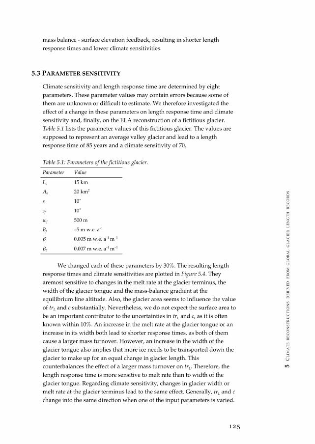
Climate sensitivity and length response time are determined by eightparameters. These parameter values may contain errors because some ofthem are unknown or difficult to estimate. We therefore investigated theeffect of a change in these parameters on length response time and climatesensitivity and, finally, on the ELA reconstruction of a fictitious glacier.Table 5.1 lists the parameter values of this fictitious glacier. The values aresupposed to represent an average valley glacier and lead to a lengthresponse time of 85 years and a climate sensitivity of 70.
Table 5.1: Parameters of the fictitious glacier.
Parameter Value
L0 15 km
A0 20 km2
s 10˚
sf 10˚
wf 500 m
Bf –5 m w.e. a–1
β 0.005 m w.e. a–1 m–1
βE 0.007 m w.e. a–1 m–1
We changed each of these parameters by 30%. The resulting lengthresponse times and climate sensitivities are plotted in Figure 5.4. Theyaremost sensitive to changes in the melt rate at the glacier terminus, thewidth of the glacier tongue and the mass-balance gradient at theequilibrium line altitude. Also, the glacier area seems to influence the valueof trL and c substantially. Nevertheless, we do not expect the surface area tobe an important contributor to the uncertainties in trL and c, as it is oftenknown within 10%. An increase in the melt rate at the glacier tongue or anincrease in its width both lead to shorter response times, as both of themcause a larger mass turnover. However, an increase in the width of theglacier tongue also implies that more ice needs to be transported down theglacier to make up for an equal change in glacier length. Thiscounterbalances the effect of a larger mass turnover on trL. Therefore, thelength response time is more sensitive to melt rate than to width of theglacier tongue. Regarding climate sensitivity, changes in glacier width ormelt rate at the glacier terminus lead to the same effect. Generally, trL and cchange into the same direction when one of the input parameters is varied.
126
60
80
100
120
140
-30 -20 -10 0 10 20 30
L0
A0
s
sf
Le
ng
th r
esp
on
se t
ime
(yr
)
Change in parameter value (%)
a
40
60
80
100
120
-30 -20 -10 0 10 20 30
wf
Bf
β
βΕ
Clim
ate
se
nsi
tivity
Change in parameter value (%)
b
Figure 5.4: Length response time (a) and climate sensitivity (b) as function of achange in the input parameters. In (a), Bf and wf coincide. (L0: reference glacierlength, A0: reference glacier area, s: mean surface slope, sf: surface slope of theglacier snout, wf: width of glacier tongue, Bf; melt rate at the glacier terminus, βE:mass-balance gradient at the ELA, β: mass-balance gradient of the glacier).
As a second step, we determined the effect of a change in lengthresponse time and climate sensitivity on the ELA reconstruction of thisfictitious glacier. We derived historic ELAs from a (fictitious) length record,which we defined as a sine function with an amplitude (L’max) of 1.5 km anda period (P) of 300 years. Instead of smoothing this record with a Gaussianfilter and calculating the derivatives with central differences, we directlyinserted this function and its time derivative in Equation (5.2). This leads to:
E tt
P'( ) sin= −
+
λ π
ϕ2 (5.15)
where λ and ϕ are the amplitude and the phase difference of the ELA
reconstruction (see Figure 5.5) and are described by:
λ π= +
11 2
2
c
tr
PLL 'max (5.16)
127
5 C
LIM
AT
E R
EC
ON
ST
RU
CT
ION
S
DE
RIV
ED
F
RO
M G
LO
BA
L G
LA
CIE
R L
EN
GT
H
RE
CO
RD
S
ϕπ π
= −
14 2 2P
P P
trLarctan (5.17)
Figure 5.5 shows the length and the reconstructed ELA as function of time.The amplitude of the ELA reconstruction thus depends on the period of thelength record, the length response time and the climate sensitivity. Thereconstruction experiences a phase difference depending on the lengthresponse time. For very large length response times, the phase differenceapproaches 0.25P.
-2
-1.5
-1
-0.5
0
0.5
1
1.5
2
-60
-45
-30
-15
0
15
30
45
60
0 50 100 150 200 250 300
L'(
t) (
km)
E'(t) (m
)
Time (a)
L' (t) E' (t)
ϕ
L'max
λ
Figure 5.5: Length record and reconstructed ELAs of the fictitious glacier. Thelength response time is 85 years and the climate sensitivity 70.
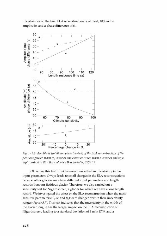
We varied the length response time between 65 and 123 years and theclimate sensitivity between 53 and 101. These numbers are the limits set bya change of 25% (plus or minus) in the most sensitive parameter, Bf (Figure5.4). The effects on the amplitude and phase difference of the ELAreconstruction are plotted in Figure 5.6. The amplitude varies roughly from30 to 59 m and the phase difference from 18 to 30 years. Note that anincrease in trL leads to larger amplitudes and an increase in c to loweramplitudes. The total effect on the ELA reconstruction constitutes the sumof both, and is therefore smaller than the individual effects. Figure 5.6cshows that the total effect on the amplitude of the ELA reconstruction is atmaximum 10%, when the melt rate at the glacier tongue is varied by 25%.
Based on this sensitivity test, we conclude that the length responsetime and the climate sensitivity are most sensitive to uncertainties in thewidth of the glacier tongue, the melt rate at the glacier snout and the mass-balance gradient at the equilibrium line altitude. The effect of these
128
uncertainties on the final ELA reconstruction is, at most, 10% in theamplitude, and a phase difference of 6.
30
35
40
45
50
55
60
70 80 90 100 110 120
Am
plitu
de (
m)
ph
ase
diff
ere
nce
(a
)
Length response time (a)
a
λ
ϕ
30
35
40
45
50
55
60
60 70 80 90 100Climate sensitivity
b
λ
ϕ
Am
plitu
de (
m)
ph
ase
diff
ere
nce
(a
)
35
40
45
50
-20 -10 0 10 20Am
plitu
de (
m)
Percentage change in Bf
c
λ
Figure 5.6: Amplitude (solid) and phase (dashed) of the ELA reconstruction of thefictitious glacier, when trL is varied and c kept at 70 (a), when c is varied and trL iskept constant at 85 a (b), and when Bf is varied by 25% (c).
Of course, this test provides no evidence that an uncertainty in theinput parameters always leads to small changes in the ELA reconstructionsbecause other glaciers may have different input parameters and lengthrecords than our fictitious glacier. Therefore, we also carried out asensitivity test for Nigardsbreen, a glacier for which we have a long lengthrecord. We investigated the effect on the ELA reconstruction when the mostsensitive parameters (Bf, wf and βE) were changed within their uncertainty
ranges (Figure 5.7). This test indicates that the uncertainty in the width ofthe glacier tongue has the largest impact on the ELA reconstruction ofNigardsbreen, leading to a standard deviation of 4 m in E’(t), and a
129
5 C
LIM
AT
E R
EC
ON
ST
RU
CT
ION
S
DE
RIV
ED
F
RO
M G
LO
BA
L G
LA
CIE
R L
EN
GT
H
RE
CO
RD
S
maximum deviation in the ELA of 9 m for the ELA maximum, whichoccurred in 1978.
-60
-40
-20
0
20
40
60
80
1750 1800 1850 1900 1950
referenceb
E ± 0.001
Bf ± 1
wf ± 100
Cha
nge
in E
LA (
m)
Year
Figure 5.7: ELA reconstruction for Nigardsbreen for different values of the inputparameters.
5.4 CASE STUDY: EUROPEAN GLACIERS
We tested the analytical model on length records of seventeenEuropean glaciers (Figure 5.1). The length response times and climatesensitivities calculated from Equations (5.9) and (5.10) were compared tovalues derived from numerical flowline models (Section 5.4.1). The ELAreconstructions, which are presented in Section 5.4.2, were compared toreconstructions derived from numerical models and from temperature andprecipitation records (Section 5.4.3).
5.4.1 LENGTH RESPONSE TIME AND CLIMATE-SENSITIVITY RESULTS
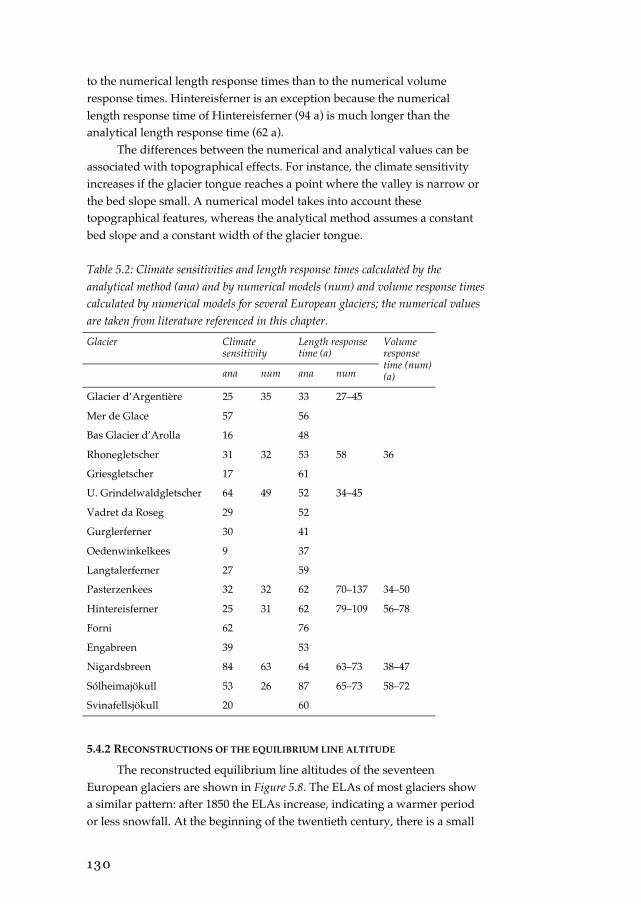
Table 5.2 shows the length response times and the climate sensitivitiesfor the seventeen European glaciers calculated with the analytical model.For some glaciers the climate sensitivity, the length response time and thevolume response time calculated with numerical models are given. Theanalytical length response times were expected to be shorter than thenumerical length response times because the analytical length responsetime is in fact a volume response time (see Section 5.2.2). However, theresults indicate that the analytical length response times correspond better
130
to the numerical length response times than to the numerical volumeresponse times. Hintereisferner is an exception because the numericallength response time of Hintereisferner (94 a) is much longer than theanalytical length response time (62 a).
The differences between the numerical and analytical values can beassociated with topographical effects. For instance, the climate sensitivityincreases if the glacier tongue reaches a point where the valley is narrow orthe bed slope small. A numerical model takes into account thesetopographical features, whereas the analytical method assumes a constantbed slope and a constant width of the glacier tongue.
Table 5.2: Climate sensitivities and length response times calculated by theanalytical method (ana) and by numerical models (num) and volume response timescalculated by numerical models for several European glaciers; the numerical valuesare taken from literature referenced in this chapter.
Glacier Climatesensitivity
Length responsetime (a)
ana num ana num
Volumeresponsetime (num)(a)
Glacier d’Argentière 25 35 33 27–45
Mer de Glace 57 56
Bas Glacier d’Arolla 16 48
Rhonegletscher 31 32 53 58 36
Griesgletscher 17 61
U. Grindelwaldgletscher 64 49 52 34–45
Vadret da Roseg 29 52
Gurglerferner 30 41
Oedenwinkelkees 9 37
Langtalerferner 27 59
Pasterzenkees 32 32 62 70–137 34–50
Hintereisferner 25 31 62 79–109 56–78
Forni 62 76
Engabreen 39 53
Nigardsbreen 84 63 64 63–73 38–47
Sólheimajökull 53 26 87 65–73 58–72
Svinafellsjökull 20 60
5.4.2 RECONSTRUCTIONS OF THE EQUILIBRIUM LINE ALTITUDE
The reconstructed equilibrium line altitudes of the seventeenEuropean glaciers are shown in Figure 5.8. The ELAs of most glaciers showa similar pattern: after 1850 the ELAs increase, indicating a warmer periodor less snowfall. At the beginning of the twentieth century, there is a small
131
5 C
LIM
AT
E R
EC
ON
ST
RU
CT
ION
S
DE
RIV
ED
F
RO
M G
LO
BA
L G
LA
CIE
R L
EN
GT
H
RE
CO
RD
S
decrease in most ELAs. After that, the ELAs increase until around 1950 andthen decrease slightly. The ELA reconstructions of UntererGrindelwaldgletscher and Glacier d’Argentière are amongst the longestrecords and show very similar fluctuations. However, the amplitudes of thefluctuations differ.
The ELA reconstruction of Rhonegletscher shows a large increasebetween 1850 and 1870 compared to the other reconstructions. This strongincrease is probably an artefact of the analytical model, which uses aconstant climate sensitivity and a constant length response time. Between1850 and 1870, the terminus of Rhonegletscher rested on a small slopingsurface, much smaller than the mean slope, implying that the glacier lengthwas actually very sensitive to a change in the ELA. If a larger climatesensitivity was applied to Rhonegletscher, a smaller increase in the ELA
1600 1700 1800 1900 2000Year
U. Grindelwaldgl., SwitzerlandGlacier d'Argentière, FranceBas Glacier d'Arolla, Switzerland
Mer de Glace, FranceRhonegletscher, Switzerland
Griesgletscher, SwitzerlandVadret da Roseg, SwitzerlandOedenwinkelkees, Austia
Langtalerferner, Austria
Gurglerferner, AustriaPasterzenkees, AustriaHintereisferner, Austria
Forni, Italy
Engabreen, Norway
Nigardsbreen, Norway
Sólheimajökull, IcelandSvinafellsjökull, Iceland
E' (
unit
is 5
0 m
)
Figure 5.8: Reconstructed ELA records of seventeen European glaciers calculatedwith the analytical model.
132
would have been calculated.Hintereisferner reveals two very steep increases in the ELA after 1850,
interrupted by significantly lower ELAs at the beginning of the twentiethcentury. The total increase in the ELA of Hintereisferner is rather largecompared to other ELA reconstructions of glaciers in the Alps. Theanalytical model is probably less valid for Hintereisferner because therelative decrease in length over the total period of Hintereisferner is large:30%. The other glaciers in the Alps retreated on average 18%.
Sólheimajökull’s high ELAs around 1760 and low ELAs just before1800 are necessary to explain its enormous retreat before and growth after1780. Svinafellsjökull, however, does not show low ELAs before 1800. Still,the large ELA fluctuations of Sólheimajökull fit with documented changesin the Icelandic climate and sea ice extent (Ogilvie, 1992): during the 1780s,sea ice remained unusually close to Iceland. Besides, the large ELAfluctuations are confirmed by ELA reconstructions of Mackintosh and
Dugmore (2000) that were calculated for Sólheimajökull with a numericalflowline model.
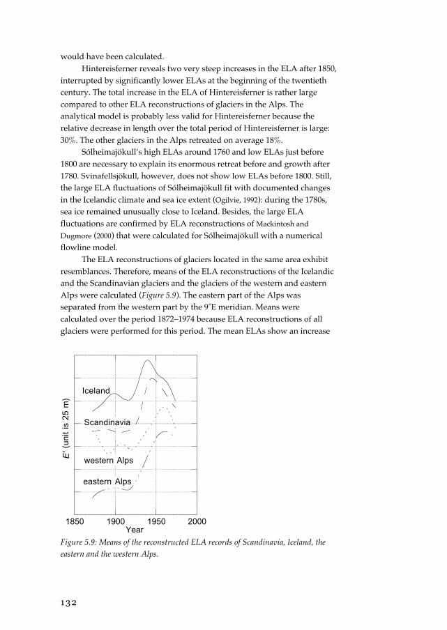
The ELA reconstructions of glaciers located in the same area exhibitresemblances. Therefore, means of the ELA reconstructions of the Icelandicand the Scandinavian glaciers and the glaciers of the western and easternAlps were calculated (Figure 5.9). The eastern part of the Alps wasseparated from the western part by the 9˚E meridian. Means werecalculated over the period 1872–1974 because ELA reconstructions of allglaciers were performed for this period. The mean ELAs show an increase
1850 1900 1950 2000
E'
(uni
t is
25
m)
Year
Iceland
Scandinavia
western Alps
eastern Alps
Figure 5.9: Means of the reconstructed ELA records of Scandinavia, Iceland, theeastern and the western Alps.
133
5 C
LIM
AT
E R
EC
ON
ST
RU
CT
ION
S
DE
RIV
ED
F
RO
M G
LO
BA
L G
LA
CIE
R L
EN
GT
H
RE
CO
RD
S
after 1915. This is 45 m for the Icelandic glaciers, 59 m for the Scandinavianglaciers, 47 m for the western Alps and 64 m for the eastern Alps.Apparently, air temperatures and snowfall have changed more in theeastern Alps than in the western Alps. The ELAs in northern Europereached a maximum before 1950 and then decreased, unlike the ELAs of theAlps, which were at maximum after 1950 and show a smaller decrease afterthat. Furthermore, it is striking that the ELAs in the western Alps were alsoat a minimum before 1900, unlike the other ELA reconstructions.
5.4.3 COMPARISON OF THE RESULTS WITH OTHER RECORDS
It would be ideal to compare the ELA reconstructions with longrecords of ELA or mass-balance observations. However, these longobservation records do not exist. Therefore, the results of the analyticalmodel were compared with different types of data: results from a simplemethod and from a numerical model and from historical temperature andprecipitation records.
Haeberli and Hoelzle (1995) calculated the average change in the massbalance over 1850–1970 from 13 length records of glaciers in the Alps. Theyassumed that the glaciers were stationary at the beginning and at the end ofthis period, and between 1890 and 1925. Subsequently, they supposed that afull dynamic response to a step change in the mass balance would explainthe glaciers’ retreat over these period. They then calculated an average massloss of –0.33±0.09 m w.e. a–1 during 1850–1970. Mass-balance changes overthe same period were also calculated for the glaciers in the Alps with theanalytical model. The average of the mass-balance changes resulted in –0.21± 0.16 m w.e a–1, which is smaller compared to the step change in massbalance calculated by Haeberli and Hoelzle. The difference between theresults of the two methods could be explained by the different approaches.First, the analytical model takes into account the response time and does notassume steady state situations before 1850 and after 1970. Second, Haeberliand Hoelzle use Equation (5.11) to determine the climate sensitivity of aglacier, which underestimates the climate sensitivity.
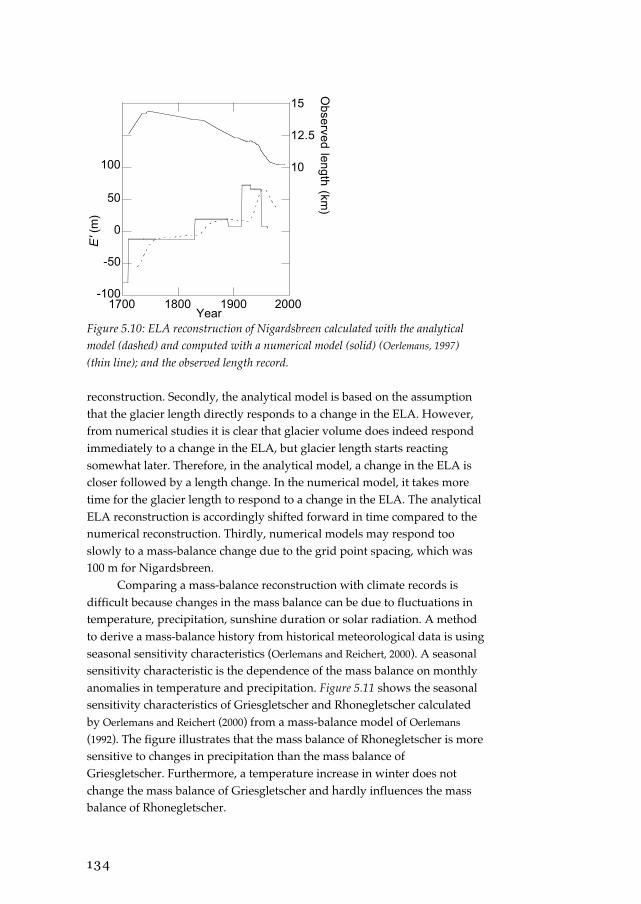
Figure 5.10 shows how the analytical ELA reconstruction ofNigardsbreen compares to the ELA reconstruction calculated from anumerical model (Oerlemans, 1997). The variation in the ELA reconstructionsis of the same size, but there is a phase difference between the tworeconstructions. Although the time at which the ELAs start to decrease orincrease is similar, the locations of the maxima and minima differ. Firstly,this difference could be due to the numerical model, which uses asuccession of step functions. Nine step functions were used to obtain thenumerical ELA reconstruction as shown in Figure 5.10. Increasing thenumber of step functions will certainly influence the ELA reconstructionand probably lead to a reconstruction that is closer to the analytical
134
-100
-50
0
50
100 10
12.5
15
1700 1800 1900 2000
E' (
m)
Ob
serve
d le
ng
th (km
)Year
Figure 5.10: ELA reconstruction of Nigardsbreen calculated with the analyticalmodel (dashed) and computed with a numerical model (solid) (Oerlemans, 1997)(thin line); and the observed length record.
reconstruction. Secondly, the analytical model is based on the assumptionthat the glacier length directly responds to a change in the ELA. However,from numerical studies it is clear that glacier volume does indeed respondimmediately to a change in the ELA, but glacier length starts reactingsomewhat later. Therefore, in the analytical model, a change in the ELA iscloser followed by a length change. In the numerical model, it takes moretime for the glacier length to respond to a change in the ELA. The analyticalELA reconstruction is accordingly shifted forward in time compared to thenumerical reconstruction. Thirdly, numerical models may respond tooslowly to a mass-balance change due to the grid point spacing, which was100 m for Nigardsbreen.
Comparing a mass-balance reconstruction with climate records isdifficult because changes in the mass balance can be due to fluctuations intemperature, precipitation, sunshine duration or solar radiation. A methodto derive a mass-balance history from historical meteorological data is usingseasonal sensitivity characteristics (Oerlemans and Reichert, 2000). A seasonalsensitivity characteristic is the dependence of the mass balance on monthlyanomalies in temperature and precipitation. Figure 5.11 shows the seasonalsensitivity characteristics of Griesgletscher and Rhonegletscher calculatedby Oerlemans and Reichert (2000) from a mass-balance model of Oerlemans
(1992). The figure illustrates that the mass balance of Rhonegletscher is moresensitive to changes in precipitation than the mass balance ofGriesgletscher. Furthermore, a temperature increase in winter does notchange the mass balance of Griesgletscher and hardly influences the massbalance of Rhonegletscher.
135
5 C
LIM
AT
E R
EC
ON
ST
RU
CT
ION
S
DE
RIV
ED
F
RO
M G
LO
BA
L G
LA
CIE
R L
EN
GT
H
RE
CO
RD
S
-0.08 -0.06 -0.04 -0.02 0 0.02 0.04123
456789
101112
dB/dT (m w.e. K-1)
Mon
th
dB/dP (m w.e. 10-1)
a: Griesgletscher
-0.08 -0.06 -0.04 -0.02 0 0.02 0.041
234
567
89
10
1112
dB/dT (m w.e. K-1)
Mon
th
dB/dP (m w.e. 10-1)
b: Rhonegletscher
Figure 5.11: Seasonal sensitivity characteristics of Griesgletscher (a) andRhonegletscher (b) calculated from a mass-balance model (Oerlemans and Reichert,
2000).
1875 1900 1925 1950 1975
B'
(un
it is
0.1
m w
.e.
a-1)
Year
Griesgletscher
Rhone-gletscher
western Alps
Figure 5.12: Mean mass-balance reconstruction of glaciers in the western Alps(dashed) and mass-balance reconstructions calculated with seasonal sensitivitycharacteristics of Griesgletscher (dotted) and Rhonegletscher (solid). A Gaussianfilter is applied to the mass-balance reconstructions.
Mass-balance reconstructions of these two glaciers in the Alps werecalculated from the seasonal sensitivity characteristics and compared withthe reconstructions calculated with the analytical model. Therefore, longrecords of monthly precipitation and temperature anomalies were needed.The monthly precipitation of Beatenberg (Switzerland) and the monthlyhomogenised high-elevation (above 1500 m a.s.l.) temperature record of 46˚
136
N, 8˚ E taken from Böhm et al. (2001) were used for both glaciers. The mass-balance reconstructions calculated from the seasonal sensitivitycharacteristics were then filtered with a Gaussian filter.
The mass-balance reconstructions of Griesgletscher and Rhone-gletscher and the mean mass-balance history of the glaciers of the westernpart of the Alps calculated with the analytical model are shown in Figure5.12. The mass-balance reconstructions show similar fluctuations withamplitudes of similar magnitude. However, there is again a phasedifference between the reconstructions. The analytical mass-balancereconstruction is shifted about 10 years forward in time, which is less thanthe phase difference between the analytical and the numerical modelresults.
5.5.4 CONCLUSIONS OF THE CASE-STUDY
Application of the analytical model to seventeen European glaciersshows that the model is useful to derive a climate signal from a glacierlength record. The calculated mass-balance fluctuations are in agreementwith mass-balance reconstructions derived from numerical models andfrom temperature and precipitation records using seasonal sensitivitycharacteristics. The length response times and climate sensitivitiescalculated with the analytical model are in agreement with valuescalculated from numerical models.
However, the ELA reconstructions calculated with the analyticalmodel are shifted forward in time by a decade compared to the numericalmass-balance reconstruction and the mass-balance reconstructionscalculated from temperature and precipitations records. This is due to themodel assumption that glacier length immediately responds to a change inthe mass balance. Another limitation of the model is that topography isrepresented in a schematic way. The topography is especially importantwhen the slope of the bedrock and the valley width change along theglacier. Then, the climate sensitivity and the length response time dependconsiderably on the position of the terminus, which in turn will influencethe mass-balance reconstruction. Therefore, the analytical model is notsuitable for glaciers with strong variations in the slope and width of theglacier valley.
5.5 GLOBAL GLACIERS AND THEIR LENGTH RECORDS
Building a data set of useful length records of worldwide glaciers wasdifficult because most non-European glaciers have only been measuredsince the beginning of the twentieth century. We aimed to find records thatgo back to before 1900. A second demand of our data set was that the length
137
5 C
LIM
AT
E R
EC
ON
ST
RU
CT
ION
S
DE
RIV
ED
F
RO
M G
LO
BA
L G
LA
CIE
R L
EN
GT
H
RE
CO
RD
S
fluctuations needed to be small (< ~20%) compared to the total glacierlength, to justify the assumption of a quasi-linear response. Thirdly, theglacier type was bound to be valley or outlet. Lastly, we neededinformation about the geometry and the mass balance to calculate theresponse time and the climate sensitivity. This led to a collection of fourteenglaciers from countries other than European, to which we added fiveEuropean records to obtain a global picture (Figure 5.13).
The glaciers of our data set are located in six regions: Canada, U.S.A.,South America, Europe, Asia and New Zealand. All of them have retreatedover the previous century, but 60% of them also slightly advanced
1600 1650 1700 1750 1800 1850 1900 1950 2000
Gla
cie
r le
ng
th (
un
it is
1 k
m)
Year
ClendenningHavocAthabasca
White GlacierBlue GlacierSouth Cascade
Frías GlacierSan Quintín
SørbreenNigardsbreen
Glacier d'Argentière
MorteratschgletscherPasterzenkees
MarukskiyBezengiGergetiSofiyskiy
Fox Glacier
Franz Josef Glacier
Figure 5.13: Glacier length fluctuations of the nineteen glaciers of our data set.
138
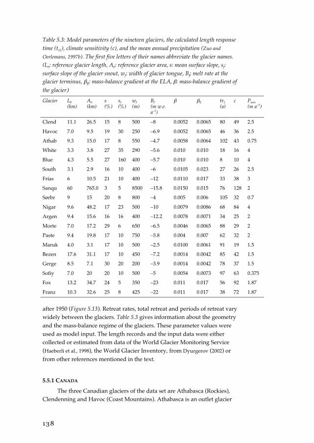
Table 5.3: Model parameters of the nineteen glaciers, the calculated length responsetime (trL), climate sensitivity (c), and the mean annual precipitation (Zuo and
Oerlemans, 1997b). The first five letters of their names abbreviate the glacier names.(L0: reference glacier length, A0: reference glacier area, s: mean surface slope, sf:surface slope of the glacier snout, wf: width of glacier tongue, Bf; melt rate at theglacier terminus, βΕ: mass-balance gradient at the ELA, β: mass-balance gradient ofthe glacier)
after 1950 (Figure 5.13). Retreat rates, total retreat and periods of retreat varywidely between the glaciers. Table 5.3 gives information about the geometryand the mass-balance regime of the glaciers. These parameter values wereused as model input. The length records and the input data were eithercollected or estimated from data of the World Glacier Monitoring Service(Haeberli et al., 1998), the World Glacier Inventory, from Dyurgerov (2002) orfrom other references mentioned in the text.
5.5.1 CANADA
The three Canadian glaciers of the data set are Athabasca (Rockies),Clendenning and Havoc (Coast Mountains). Athabasca is an outlet glacier
139
5 C
LIM
AT
E R
EC
ON
ST
RU
CT
ION
S
DE
RIV
ED
F
RO
M G
LO
BA
L G
LA
CIE
R L
EN
GT
H
RE
CO
RD
S
of the Columbia Ice Field, an ice cap of roughly 325 km2. The glacier flowsover three icefalls into an alpine valley (Reynolds and Young, 1997). It hasretreated rapidly since 1910 until 1960, after which a slowdown in theretreat rate occurred. Clendenning and Havoc, two valley type glaciers, arelocated closer to the ocean and their glacier termini reach further down (±1000 m a.s.l.) than Athabasca (±1950 m a.s.l.). The length records ofClendenning and Havoc do not show similar patterns, although both arelocated in the Clendenning valley. This could be attributed to differences inglacier geometry because the glacier tongue of Havoc is much steeper andnarrower.
5.5.2 U.S.A.
White and Blue Glaciers are located in the Olympic Mountains, whichis ±55 km from the Pacific Ocean. The climate of the Olympic mountains isstrongly maritime and involves the greatest precipitation of any area in theU.S.A., excluding Alaska and Hawaii (Armstrong, 1989). Blue Glacier has asteeper and narrower glacier tongue than White Glacier and has retreatedless. South Cascade lies in the North Cascade Range, 250 km from theocean. This glacier receives less snow (±3 m w.e.) than White and BlueGlaciers (±4 m w.e.) (Rasmussen and Conway, 2001). Mass-balancemeasurements have been carried out on Blue Glacier (Conway et al., 1999)and South Cascade (Krimmel, 2000). Armstrong (1989) showed that BlueGlacier had a slightly positive mass balance between 1956 and 1986 (0.3 m)and Krimmel (1989) found a mean negative balance for South Cascade (–0.22m) for 1959 to 1985. Blue Glacier has not retreated significantly since 1950,while the length record of South Cascade shows an ongoing retreat.Rasmussen and Conway (2001) concluded that South Cascade has been moreout of balance than White Glacier, which they ascribed to differences ingeometry between the two glaciers, rather than in climate.
5.5.3 SOUTH AMERICA
Frías Glacier (Argentina) is an outlet glacier situated on the east sideof Mount Tronador. This ice cap is the northernmost ice body of Argentina.Measurements from a weather station in the Rio Frías Valley of FríasGlacier indicated that the annual precipitation amounts to 4300 mm a–1
(Perez Moreau, 1945). The glacier fluctuations have been recorded since 1976and Villalba et al. (1990) dated oscillations of Frías Glacier by using tree-ringanalysis. Between 1850 and 1900, the retreat rate was 7 m a–1 and increasedto 10 m a–1 between 1910 and 1940.
San Quintín is further south than Frías Glacier and is the largestglacier of our data set. It is a piedmont outlet glacier of the NorthPatagonian Ice Field in Chile. San Quintín flows to the west, onto an
140
outwash plain. It receives between 3700 and 6700 mm precipitation peryear. Winchester and Harrison (1996) investigated the ice front retreats andadvances and concluded that precipitation is the main factor controlling thefluctuations. The length record of San Quintín shows a peculiar glacierretreat just before 1935 from which it recovers after 1935, which does notshow up in the other length records.
5.5.4 EUROPE
Sørbreen is a glacier on Jan Mayen, the northernmost island on theMid-Atlantic Ridge (71˚N, 8˚W). This glacier flows southwards to the ocean,from the 2277-m high Beerenberg volcano. The climate is cool oceanic withan annual mean air temperature of –1.2 ˚C at sea level. The island issurrounded with pack ice during winter and spring (Anda et al., 1985).Nigardsbreen is an outlet glacier in Norway, flowing from the largest icecap of continental Europe (Jostedalsbreen) in a southeasterly direction. It isa maritime glacier, located close to the Atlantic ocean. It advanced veryrapidly between 1710 and 1748 and after 1988, it slightly advanced again.Pohjola and Rogers (1997) claimed that this advance is due to enhancedwesterly maritime flow after 1980 leading to high winter accumulation andlow summer ablation.
Glacier d’Argentière (France), Morteratschgletscher (Switzerland) andPasterzenkees (Austria) are valley glaciers in the European Alps, where theclimate is more continental. Glacier d’Argentière has been documentedwell, regarding the numerous fluctuations registered before 1850. Its lengthrecord is the longest of our data set and has been studied by Huybrechts et al.
(1989). Glacier d’Argentière advanced after 1970, in contrast toMorteratschgletscher and Pasterzenkees. Pasterzenkees is the longestglacier of the Austrian Alps. It retreated roughly during two periods:between 1870 and 1910 and after 1930 (Zuo and Oerlemans, 1997a).
5.5.5 ASIA
Marukskiy, Bezengi and Gergeti are valley glaciers in the CaucasusMountains. Their length records contain only a few measurements, whichexplains the straight lines in Figure 5.13. The mass-balance gradient of theseglaciers is relatively small and the melt rate at the glacier tongue is low(Table 5.3). The maximum elevation of Bezengi and Gergeti is over 5000 ma.s.l. Sofiyskiy glacier is located in the Altai Mountains of central Asia, aborder region between Russia and Mongolia. It is a so-called continental,summer-accumulation type glacier. Sofiyskiy glacier is a valley type glacierconsisting of three basins. The most rapid retreat of Sofiyskiy glacieroccurred between 1900 and 1940 (Pattyn et al., 2003; De Smedt and Pattyn, 2003).
141
5 C
LIM
AT
E R
EC
ON
ST
RU
CT
ION
S
DE
RIV
ED
F
RO
M G
LO
BA
L G
LA
CIE
R L
EN
GT
H
RE
CO
RD
S
5.5.6 NEW ZEALAND
Fox and Franz Josef are valley glaciers in the maritime climate of theSouthern Alps of New Zealand. They receive between 5 and 15 mprecipitation per year. Their glacier tongues lie at very low elevations, 425and 305 m a.s.l. for Franz Josef and Fox Glaciers respectively (Hooker and
Fitzharris, 1999). The length records show similar patterns: a rapid retreatafter 1940 and a major advance after 1982. This advance phase ischaracterised by higher precipitation and is also related to a higherfrequency of El Niño events (Hooker and Fitzharris, 1999).
5.6 RESULTS FOR WORLDWIDE GLACIERS
5.6.1 LENGTH RESPONSE TIMES AND CLIMATE SENSITIVITIES
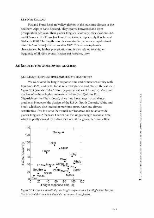
We calculated the length response time and climate sensitivity withEquations (5.9.) and (5.10) for all nineteen glaciers and plotted the values inFigure 5.14 (see also Table 5.3 for the precise values of trL and c). Maritimeglaciers often have high climate sensitivities (San Quintín, Fox,Nigardsbreen and Franz Josef), since they have large mass-balancegradients. However, the glaciers of the U.S.A. (South Cascade, White andBlue), which are also located in maritime areas, have low climatesensitivities. This is due to their small surface areas and relative wideglacier tongues. Athabasca Glacier has the longest length response time,which is partly caused by its low melt rate at the glacier terminus. Blue
0
20
40
60
80
100
120
140
0 20 40 60 80 100 120
Clim
ate
se
nsi
tivity
Length response time (a)
Athab
BezenGerge
Clend
Foxgl
Franz
Frías Havoc
Maruk
Sanqu
Sofiy
South
WhiteBlue
Nigar
ArgenPaste SørbrMorte
Figure 5.14: Climate sensitivity and length response time for all glaciers. The firstfive letters of their names abbreviate the names of the glaciers.
142
Glacier has the shortest length response time and the lowest climatesensitivity. Since this glacier is situated on a steep slope, the contribution ofthe mass balance - surface height feedback to trL and c is small.
5.6.2 ELA RECONSTRUCTIONS
Figure 5.15 shows the reconstructed ELAs. Athabasca and Havoc showsimilar fluctuations in the ELA although the ELA of Havoc started toincrease some years before 1900 and that of Athabasca some years after1900. The ELA reconstruction of Clendenning shows neither anyresemblances with the other Canadian ELAs nor with the reconstructionsfor the U.S.A. because the ELA does not stabilise around 1950. Thereconstructed ELAs of White and Blue Glaciers are similar, but thefluctuation in White Glacier’s ELA is larger.
The ELAs of Frías and San Quintín show hardly any correspondence.The ELA of San Quintín decreases exceptionally after 1920. As San Quintínis a piedmont glacier and not a valley glacier, it could be argued whether itsELA reconstruction is reliable. However, the rapid decrease could beexplained by an increase in precipitation between 1919 and 1935 (Winchester
and Harrison, 1996). Winchester and Harrison (1996) also found thatprecipitation is a more dominant factor than air temperature in controllingthe fluctuations of San Quintín.
The ELA of the European glaciers increased between 1920 and 1950.Sørbreen reached a maximum ELA before 1950 and the other glaciers after1950. Morteratschgletscher’s increase in the ELA is large compared to theother ELA reconstructions in the European Alps. Bogen et al. (1989) foundthat the increase in the ELA of Nigardsbreen that occurred between 1925and 1955 is related to a series of excessive warm summers.
Marukskij, Bezengi and Gergeti all show slowly increasing ELAs until1950–1970 and a decrease afterwards. The ELA of Sofiyskiy increasesrapidly around 1900 and starts decreasing already after 1930.
The reconstructed ELAs of Fox and Franz Josef show very similarpatterns, with a rapid increase in the ELA after 1920 until 1960. The highELAs around 1960 are strongly linked with changes in the circulationpatterns over the southwest Pacific region (Fitzharris et al., 1992). At that time,summer pressures over New Zealand were higher than normal due to apole-ward shift of the subtropical high, favoring clearer skies and moreablation. Moreover, snow accumulation was unusually low in the 1960s and1970s.
5.6.3 WORLDWIDE PATTERN IN ELA FLUCTUATIONS
For all glaciers, ELA reconstructions were calculated for the periodbetween 1910 and 1959. We therefore estimated an average worldwide
143
5 C
LIM
AT
E R
EC
ON
ST
RU
CT
ION
S
DE
RIV
ED
F
RO
M G
LO
BA
L G
LA
CIE
R L
EN
GT
H
RE
CO
RD
S
-60
-30
0
30
60
90
120
1800 1850 1900 1950 2000
ClendHavocAthab
Cha
nge
in E
LA (
m)
Year
Canada
-60
-30
0
30
60
90
120
1800 1850 1900 1950 2000
WhiteBlueSouth
Cha
nge
in E
LA (
m)
Year
U.S.A.
-60
-30
0
30
60
90
120
1800 1850 1900 1950 2000
FríasSanqu
Cha
nge
in E
LA (
m)
Year
South America
-60
-30
0
30
60
90
120
1800 1850 1900 1950 2000
SørbrNigarArgenMortePaste
Cha
nge
in E
LA (
m)
Year
Europe
-60
-30
0
30
60
90
120
1800 1850 1900 1950 2000
MarukBezenGergeSofiy
Cha
nge
in E
LA (
m)
Year
Asia
-60
-30
0
30
60
90
120
1800 1850 1900 1950 2000
FoxglFranz
Cha
nge
in E
LA (
m)
Year
New Zealand
Figure 5.15: ELA reconstructions for all glaciers plotted separately for six regions.The first five letters of their names abbreviate the names of the glaciers.
144
change in the ELA for this period (Figure 5.16a). The average ELA increasedby 33 m between 1910 and 1959, with a standard error of 8 m. According toFigure 5.15, this increase was most pronounced in the U.S.A. and NewZealand and less in Asia. Generally, the reconstructed ELAs increasedstrongly during the first fifty years of the twentieth century. Except for SanQuintín, they all decreased again in the second half of the twentieth centuryuntil 1980, when most of our ELA reconstructions end. This implies that thefirst half of the twentieth century was warmer or drier than the periodbefore 1900. After 1960, the climate returned to a situation that favourslower ELAs.
1850 1870 1890 1910 1930 1950 1970
-80
-60
-40
-20
0
20
40
60
Cha
nge
in E
LA (
m)
Year
a
1850 1870 1890 1910 1930 1950 1970
-2
-1
0
1
2
Cha
nge
in t
empe
ratu
re (
K)
Year
b
Figure 5.16: (a) All ELA reconstructions (dashed) and the average ELAreconstruction (solid). The ELA reconstruction of each glacier is shifted comparedto Figure 5.15 in order to obtain a mean E’(t) of zero over the period 1910 to 1959.(b) Same as Figure 5.16a, but for temperature reconstructions.
5.6.4 RECONSTRUCTIONS OF TEMPERATURE
If we assume that the changes in the ELA were solely due totemperature variations, we can derive historic trends in air temperaturefrom the ELA reconstructions. We then only need to know the sensitivity ofthe glacier mass balance to the temperature. A change in the ELA (E’(t)) canbe easily translated into a mass-balance change (B’(t)) by multiplying it withthe mass-balance gradient. We estimated for each glacier the sensitivity ofthe mass balance to a change in temperature (T’(t)) by using aparameterisation of Oerlemans (2001):
B t
T tPann
'( )'( )
. ( ) .= −0 271 0 597(5.18)
145
5 C
LIM
AT
E R
EC
ON
ST
RU
CT
ION
S
DE
RIV
ED
F
RO
M G
LO
BA
L G
LA
CIE
R L
EN
GT
H
RE
CO
RD
S
Oerlemans (2001) based this parameterisation on calculations with a mass-balance model applied to a set of thirteen glaciers. The sensitivity is afunction of mean annual precipitation (Pann) and increases for wetterclimates. We chose, for each glacier, a value for the annual precipitation,based on the compiled data of Zuo and Oerlemans (1997b) (Table 5.3). Figure 8bshows the calculated temperature reconstructions for each glacier and anaverage temperature trend. Between 1910 and 1959, the average increase inair temperature was 0.8 K and the standard error in the mean 0.2 K. Thecalculated linear trend in temperature was 0.19 K per decade.
5.7 DISCUSSION
Our results agree with those of the IPCC (2001) on an increase in theglobal surface air temperature between 1910 and 1945 if we assume that theELA fluctuations were solely explained by changes in temperature. Inaddition, cooling during the period 1946 to 1975 in the NorthernHemisphere (IPCC, 2001) is consistent with the observed lowering in ourreconstructed ELAs. However, the warming rate reported by the IPCC forthe period 1910–1945 is less (0.14 K per decade) than estimated from theELA reconstructions for 1910 to 1959 (0.19 K per decade). This may beassociated with the fact that we excluded precipitation and cloudiness aspossible causes of the ELA fluctuations. Besides, we estimated this globaltemperature increase from only a few glacier records that are also notevenly distributed over the globe.
The IPCC also concluded that the Southern Hemisphere has beenwarming more uniformly during the twentieth century compared with theNorthern Hemisphere and shows warming between 1946 and 1975 too. Thisis in contrast with the decreasing ELAs of the glaciers in New Zealand,unless precipitation has increased simultaneously. Regional differencesfrom the hemispherical mean could also account for this discrepancy.
Our results do not give rise to the conclusion that there was a secondperiod (1976 to 2000) of global warming, as claimed by the IPCC (2001). Thisis because most of our reconstructed ELAs do not extend beyond 1980, dueto the time span of the length records and the Gaussian filter that weapplied.
As we related changes in the ELA to changes in the specific massbalance, we could as well determine the mean specific mass balance foreach glacier between 1910 and 1959. Averaged over all glaciers, this resultsin a mean specific mass balance of –0.18 m w.e. a–1 with a standard error of0.04 m w.e. a–1. If we assume this value to be representative for all glaciersin the world, the mean rise in sea level due to the retreating glaciers can beroughly estimated. Assuming an area of 527 900 km2 for all of the world’s
146
small ice caps and glaciers excluding Greenland and Antarctica (Zuo and
Oerlemans, 1997b), the estimated total rise in sea level is 1.3 cm over theperiod 1910–1959 and the mean rate is 0.3 mm a–1. This rate is in accordancewith the estimated contribution of glaciers to sea level rise for the period1910–1990 reported by the IPCC (2001). However, we should realise that thisestimate is not very accurate, as we did not include any information fromglaciers in Alaska and north-east Canada, which are highly glacierisedareas. Neither did we use a weighted average to account for the size of eachglacierised region.
5.8 SUMMARY
The purpose of this study was to extract information on the pastclimate from glacier length fluctuations by means of deriving historicalELAs or mass-balance recnstructions. The model that we developed forextracting ELAs from glacier length fluctuations is a simple analytical one,based on the assumption that the change in length can be described by alinear response equation. Its advantage is that it takes the response time andthe geometry of the glacier as well as the mass balance - surface heightfeedback into account. Furthermore, it requires less information about aglacier than is needed for a numerical model.
We carried out a sensitivity test for a fictitious glacier and found thatthe uncertainty in the width of the glacier tongue, the melt rate at the glacierterminus and the mass-balance gradient have the largest impact on the ELAreconstruction. More specifically, for Nigardsbreen, the standard deviationin the ELA reconstruction due to uncertainties in the input parameters wasestimated to be 4 m.
We performed a case-study, in which we tested the analytical modelon length records of seventeen European glaciers. The results indicate thatthe model is useful to derive a climate signal from a glacier length record.The calculated mass-balance fluctuations are in agreement with mass-balance reconstructions derived from numerical models and fromtemperature and precipitation records using seasonal sensitivitycharacteristics. However, the ELA reconstructions calculated with theanalytical model are shifted forward in time by a decade compared to thenumerical mass-balance reconstruction and the mass-balancereconstructions calculated from temperature and precipitations records. Theanalytical model is not suitable for glaciers with strong variations in theslope and width of the glacier valley and only valid for relatively smallglacier length fluctuations.
We then extracted information on the past climate from glacier lengthfluctuations for nineteen glaciers from different parts of the world. Theresults show that all glaciers of our data set experienced an increase in the
147
5 C
LIM
AT
E R
EC
ON
ST
RU
CT
ION
S
DE
RIV
ED
F
RO
M G
LO
BA
L G
LA
CIE
R L
EN
GT
H
RE
CO
RD
S
ELA between 1900 and 1960. The average increase between 1910 and 1959 is33 m. After around 1960 until 1980, the ELAs decreased to lower elevations.This implies that during the first half of the twentieth century, climate waswarmer or drier than before. The results support the evidence that anaverage global temperature increase took place between 1910 and 1945 anda sea level increase of 0.3 mm a–1 (IPCC, 2001). The ELA reconstructions alsoreveal regional differences. Changes in the ELA were most pronounced forNorth America, Europe and New Zealand. After 1960 up to 1980, theclimate reverted to conditions supporting lower ELAs.
Acknowledgements – We would like to thank Martin Hoelzle and RegulaFrauenfelder of the WGMS for providing the glacier length records,Reichert Böhm for the temperature records and Maurice Schmeits for theprecipitation record. We are grateful to a number of people who suppliedus with useful data and information on glaciers: Ricardo Villalba, MikeDemuth, Frank Pattyn, Bert De Smedt, Trevor Chinn, , Andrey Glazovskyand Al Rasmussen. We thank the members of the Ice & Climate group ofthe IMAU and and especially Wouter Greuell, Andrew Mackintosh, AlethBolt and Angelina Souren for their helpful comments.
REFERENCES
Anda, A., Orheim, O. and Mangerud, J. 1985. Late Holocene glacier variations at JanMayen. Polar Research, 3 n.s., 129–140.
Aniya, M. 1999. Recent glacier variations of the Hielos Patagónicos, South America,and their contribution to sea–level change. Arctic, Antarctic and Alpine Research,31(2), 165–173.
Armstrong, R.L. 1989. Mass balance history of Blue Glacier, Washington, USA. InOerlemans, J., editor, Glacier fluctuations and climatic change, Dordrecht: KluwerAcademic Publishers, 183–192.
Benn, D.I. and Lehmkuhl, F. 2000. Mass balance and equilibrium–line altitudes ofglaciers in high–mountain environments. Quaternary International, 65/66, 15–29.
Bogen, J., Wold, B. and Østrem, G. 1989. Historic glacier variations in Scandinavia. InOerlemans, J., editor, Glacier fluctuations and climatic change, Dordrecht: KluwerAcademic Publishers: 109–128.
Böhm, R., Auer, I., Brunetti, M., Maugeri, M., Nanni, T. and Schöner, W. 2001.Regional temperature variability in the European Alps 1760–1980 fromhomogenized instrumental time series. International Journal of Climatology,21(14), 1779–1801.
Callendar, G.S. 1950. Note on the relation between the height of the firn line anddimensions of a glacier. Journal of Glaciology, 1(8), 459–461.
Chinn, T.J. 1996. New Zealand glacier responses to climate change of the pastcentury. New Zealand Journal of Geology and Geophysics, 39, 415–428.
Conway, H., Rasmussen, L.A., Marshall, H.P. 1999. Annual mass balance of Blueglacier, U.S.A.: 1955–97. Geografiska Annaler, 81A(4), 509–520.
148
De Smedt, B. and Pattyn, F. 2003. Numerical modelling of historical front variationsand dynamic response of Sofiyskiy Glacier, Altai Mountains, Russia. Annals ofGlaciology, 37: in press.
Dyurgerov, M.B. 2002. Glacier mass balance and regime: data of measurements andanalysis. In: Meier, M. F. and Armstrong, R. (Eds.), Occasional Paper, vol. 55.Institute of Arctic and Alpine Research, University of Colorado, Boulder, CO,88 pp.
Fitzharris, B.B., Hay, J.E. and Jones, P.D. 1992. Behaviour of New Zealand glaciersand atmospheric circulation changes over the past 130 years. The Holocene, 2(2),97–106.
Greuell, W. 1992. Hintereisferner, Austria: mass balance reconstruction andnumerical modelling of the historical length variations. Journal of Glaciology,38(129), 233–244.
Haeberli, W. and Hoelzle., M. 1995. Application of inventory data for estimatingcharacteristics of and regional climate-change effects on mountain glaciers: apilot study with the European Alps. Annals of Glaciology, 21, 206–212.
Haeberli, W., Hoelzle, M., Suter, S., and Frauenfelder, R., editors 1998. Fluctuations ofglaciers 1990–1995. Paris: IAHS/UNESCO.
Hoelzle, M., Haeberli, W., Dischl, M., and Peschke, W. 2003. Secular glacier massbalances derived from cumulative glacier length changes. Global and PlanetaryChange, 790, 1–12.
Hooker, B.J., and Fitzharris, B.B. 1999. The correlation between climatic parametersand the retreat and advance of Franz Josef Glacier, New Zealand. Global andPlanetary Change, 22, 39–48.
Huybrechts, P., de Nooze, P., and Decleir, H. 1989. Numerical modelling of Glacierd’Argentière and its historic front variations. In Oerlemans, J., editor, Glacierfluctuations and climatic change, Dordrecht: Kluwer Academic Publishers,373–389.
IPCC, 2001. Climate Change 2001; The Scientific Basis. Contribution of Working Group Ito the Third Assessment Report of the Intergovernmental Panel on ClimateChange. Cambridge University Press, Cambridge, United Kingdom and NewYork, NY, USA, 881 pp.
Jóhannesson, T., Raymond, C. and Waddington, E. 1989. Time-scale for adjustment ofglaciers to changes in mass balance. Journal of Glaciology, 35(121), 355–369.
Kaser, G. 1999. A review of the modern fluctuations of tropical glaciers. Global andPlanetary Change, 22, 93–103.
Krimmel, R.M. 1989. Mass balance and volume of South Cascade Glacier,Washington 1958–1985. In Oerlemans, J. (ed.), Glacier fluctuations and climaticchange, Dordrecht: Kluwer Academic Publishers, 193–206.
Krimmel, R.M. 2000. Water, Ice and Meteorological Measurements at South CascadeGlacier, Washington, 1999 Balance Year. USGS WRI-00-4139.
Mackintosh, A.N. and Dugmore, A.J. 2000. Modelling Holocene glacier fluctuationsand climatic change in Iceland. Geolines, 11, 142–146.
Mackintosh, A.N. 2000. Glacier fluctuations and climatic change in Iceland. Ph.D. Thesis,Department of Geography, University of Edinburgh, Scotland.
Manley, G. 1959. The late-glacial climate of north-west England. Liverpool andManchester Geological Journal, 2, 188–215.
Meierding, T.C. 1982. Late Pleistocene glacial equilibrium-line in the Colorado FrontRange: A comparison of methods. Quaternary Research, 18, 289–310.
149
5 C
LIM
AT
E R
EC
ON
ST
RU
CT
ION
S
DE
RIV
ED
F
RO
M G
LO
BA
L G
LA
CIE
R L
EN
GT
H
RE
CO
RD
S
Nye, J.F. 1965. A numerical method of inferring the budget history of a glacier fromits advance and retreat. Journal of Glaciology, 35(121), 355–369.
Oerlemans, J. 1992. Climate sensitivity of glaciers in southern Norway: application ofan energy-balance model to Nigardsbreen, Hellstugubreen and Alfotbreen.Journal of Glaciology, 38(129), 223–232.
Oerlemans, J. 1994. Quantifying global warming from the retreat of glaciers. Science,264, 243–245.
Oerlemans, J. 1997. A flowline model for Nigardsbreen, Norway: projection of futureglacier length based on dynamic calibration with the historic record. Annals ofGlaciology, 24, 382–389.
Oerlemans, J. and Reichert, B.K. 2000. Relating glacier mass balance to meteorologicaldata by using a seasonal sensitivity characteristic. Journal of Glaciology, 46(152),1–6.
Oerlemans, J. 2001. Glaciers and Climate Change. Rotterdam, A.A. Balkema Publishers,148 pp.
Ogilvie, A. 1992. Documentary evidence for changes in the climate AD 1500–1800. InBradley, R. and Jones, P., editors, Climate since AD 1500 , London: Routdledge,92–117.
Paterson, W.S.B. 1994. The physics of glaciers. Third edition. Oxford: Elsevier.Pelfini, M. and Smiraglia, C. 1997. Signals of 20th-century warming from the glaciers
in the Central Italian Alps. Annals of Glaciology, 24, 350–354.Pattyn, F., De Smedt, B., De Brabander, S., Van Huele, W., Agatova, A., Mistrukov,
A., and Decleir, H. 2003. Ice dynamics and basal properties of SofiyskiyGlacier, Altai Mountains, Russia based on DGPS and radio-echo soundingsurveys. Annals of glaciology, 37: in press.
Pelto, M.S. and Hedlund, C. 2001. Terminus behavior and response time of NorthCascade glaciers, Washington, U.S.A. Journal of Glaciology, 47(158), 497–506.
Perez Moreau, R.A. 1945. Reseña Botánica sobre los Parques Nacionales NahuelHuapi, Los Alerces y Lanín. Anales del Museo de la Patagonia, 1, 253–276.
Pohjola, V.E. and Rogers, J.C. 1997. Atmospheric circulation and variations inScandinavian glacier mass balance. Quaternary Research, 47, 29–36.
Porter, S.C. 1975. Equilibrium-line altitudes of late Quaternary glaciers in theSouthern Alps, New Zealand. Quaternary Research, 5, 27–47.
Rasmussen, L.A. and Conway, H. 2001. Estimating South Cascade Glacier(Washington, U.S.A.) mass balance from a distant radiosonde and comparisonwith Blue glacier. Journal of Glaciology, 47(159), 579–588.
Reynolds, J.R. and Young, G.J. 1997. Changes in areal extent, elevation and volume ofAthabasca Glacier, Alberta, Canada, as estimated from a series of mapsproduced between 1919 and 1979. Annals of Glaciology, 24, 60–65.
Savoskul, O.S. 1997. Modern and Little Ice Age glaciers in ‘humid’ and ‘arid’ areas ofthe Tien Shan, Central Asia: two different patterns of fluctuation. Annals ofGlaciology, 24, 142–147.
Schmeits, M.J. and Oerlemans, J. 1997. Simulation of the historical variation in lengthof the Unterer Grindelwaldgletscher, Switzerland. Journal of Glaciology, 43(143),152–164.
Solomina, O.N. 2000. Retreat of mountain glaciers of northern Eurasia since the LittleIce Age maximum. Annals of Glaciology, 31, 26–30.
150
Villalba, R., Leiva, J.C., Rubulls, S., Suarez, J., and Lenzano, L. 1990. Climate, tree-ring, and glacial fluctuations in the Rio Frías valley, Rio Negro, Argentina.Arctic and Alpine Research, 22(3), 215–232.
Wallinga, J. and Van de Wal, S.W. 1998. Sensitivity of Rhonegletscher, Switzerland, toclimate change: experiments with a one-dimensional flowline model. Journal ofGlaciology, 44(147), 383–393.
Warren, C.R. and Sugden, D.E. 1993. The Patagonian Icefields: A glaciological review.Arctic and Alpine Research, 25(4), 316–331.
Winchester, V. and Harrison, S. 1996. Recent oscillations of the San Quintín and SanRafael glaciers, Patagonian Chile. Geografiska Annaler, 78A, 35–49.
Zuo, Z. and Oerlemans, J. 1997a. Numerical modelling of the historic front variationand the future behaviour of the Pasterze glacier, Austria. Annals of Glaciology,24, 234–241.
Zuo, Z. and Oerlemans, J. 1997b. Contribution of glacier melt to sea-level rise sinceAD 1865: a regionally differentiated calculation. Climate Dynamics, 13, 835–845.