5 distribution, inventory and condition · chapter 5: distribution, inventory and condition 253 5.2...

chapter 5: distribution, inventory and condition 251

5 distribution, inventory and condition

5.1 Mappingmangroveandcoastalsaltmarsh–abackground

issues associated with mapping vegetation and preparation of inventories

Vegetation mapping and inventory are important for many reasons. The maps produced from this project, for example, are likely to be used for multiple purposes:• Atoolformanagers. Vegetation maps are routinely used by land managers who wish to select and locate

places to carry out actions (weeding, fencing, etc.).• Toassistwithmonitoring. Changes in vegetation can be perceived and quantified if baseline vegetation

maps exist which describe a former state. For effective monitoring to be achieved, successive maps must have comparable information (e.g. typology) and be resolved at a scale sufficient to show any changes. We stress that, while our maps may be suitable for monitoring changes on a state- and catchment-wide scale over decadal time scales, they are not suitable to track more subtle changes within individual patches of saltmarsh or over short periods of time. We use reconstructed pre-colonial maps to quantify long-term changes in mangroves and coastal saltmarsh in Chapter 6.1.

• Tosupportplanningandpolicy. In order to develop effective conservation strategies, policymakers must know the extent and type of vegetation, how it is distributed across land tenures, what threats it faces, and how depleted it has become. In Victoria, vegetation maps underpin the operation of Victoria’s Native Vegetation Management Framework (Department of Sustainability and Environment 2002b).

• Asaninputtofutureresearch. Vegetation maps are routinely used by researchers, and may be used to stratify a sampling strategy; to extract ‘habitat’ information for sites of interest, or as inputs into spatial models of species habitat.

• Asaneducationaltool. Vegetation maps help us appreciate and interpret pattern. They can be used to elucidate ecological processes and demonstrate biological diversity.

This multiplicity of potential uses imposes a number of theoretical and practical constraints on the production and interpretation of vegetation maps. Among the most important relate to typology (discussed in Chapter 4), scale, presentation, temporal change and the choice of data format.

Scale is a critically important concept in ecology because different processes and spatial patterns become manifest (or obscured) at different spatial resolutions. In fact, Levin (1992) argued that the problem of scale was a ‘fundamental question in ecology’. Scale presents a particular problem when examining the patchy distribution of plants across space and constructing vegetation maps, because decisions must be made as to when and how we decide what level of patchiness is meaningful for describing vegetation and what constitutes ‘noise’. This is a difficult question of persistent relevance (Whitaker 1975; Turner et al. 1989; Levin 1992). It is clear, however, that there is no single ‘correct’ scale for describing a landscape, as different portions of the landscape can display more or less intricate patterning of vegetation. Scale is a problem also for the calculation of areas and for indices of connectivity (Turner et al. 1989): as resolution changes, patches appear and disappear. That phenomenon cannot be solved, but must be recognised as an inevitable source of error in all area statistics.

Second, the bounds of some vegetation types (here EVCs) are more finely resolved than others. In theory, vegetation maps would show ‘fuzzy’ zones of transition, some wide, some narrow. The problem is that the EVC typology and the policy mechanisms which deal with vegetation in Victoria (and elsewhere) are not

mangroves and coastal saltmarsh of victoria: distribution, condition, threats and management252

fuzzy; nor is the software used by most agencies capable of representing such subtleties. The use of complexes and mosaics (discussed below) is the only ‘semi-fuzzy’ concession, given these constraints. Flagging this issue of the fuzzy nature of vegetation categories and boundaries to data-users is perhaps the only practical solution.

Temporal change is the third issue that requires consideration. Vegetation maps are a snapshot in time; in real life, however, vegetation extent, condition and type all change on different temporal scales. The issue then becomes: ‘How long will it take before the dataset is no longer a reliable picture of current pattern?’ Change in vegetation occurs patchily across the state, through processes such as gradual invasion by weeds, catastrophic changes such as clearing (Department of Sustainability and Environment 2008), and the shifting patterns of ecological gradients (such changes are described in the analysis of climate change impacts in Chapter 6.2). In principle, it would be possible to calculate the rate at which the accuracy of maps decays, but that is impractical within the scope of the current project. More importantly, however, such a ‘rate of decay’ affects future management decisions, which may be influenced by policy and socio-economic factors, not by mapping techniques or data quality and availability. Such constraints must be recognised by the users of any vegetation map.

overview of technical methods for mapping coastal vegetation

There are many ways to create a vegetation map, including:• Remote sensing and modelling, where imagery is analysed to define zones using an automatic process.• Aerial photograph interpretation (API), where photographs are interpreted by experts and the vegetation

patterns are ‘traced’.• Field work (‘ground truthing’), where areas are visited in person to examine the vegetation.

The three approaches may not be mutually exclusive. Remote sensing, for example, usually requires field work to determine what the recognisable zones represent ‘on-ground’; in turn, field work is often best guided by aerial photographs of the area in question.

Given the suite of approaches theoretically available for mapping, several practical constraints influenced the approach we developed for Chapter 5:• Needforconsistencyandreliabilityatmultiplescales. Our data will be used for statewide planning

purposes, where the statewide pattern is of primary importance and the intricate detail is largely irrelevant. The data will be used also for some site-scale purposes, where each polygon boundary may have some significance, but inconsistencies between regions are not highly important. It is difficult to manage both uses simultaneously.

• Limitationsoftheexistingaerialphotographresource. As funds were not available to fly new photographic runs specifically for the project, existing maps had to be utilised. The existing state government resource is good, but it varies in resolution, as well as the season and time of day images were taken. Seasonal and diurnal variations make it difficult to achieve consistent, statewide coverage with the existing aerial photographs.

• Timeandresourceconstraints. The project’s short duration and limited funding did not allow every saltmarsh in Victoria to be visited ‘on the ground’ and its vegetation examined in detail.

• ConsistencywithexistingmapdatasetsheldbytheDepartmentofSustainabilityandEnvironment. Since the mapping and inventory information will be used in the Victorian policy and management context, the dataset needs to be in the form of attributed polygons on a geographic information system (GIS).


5.2 Methodsusedtomapcurrentextentofmangrovesandcoastalsaltmarsh

Given the constraints noted above, we decided to use a mapping approach which combined extensive field work and onsite aerial photograph interpretation and annotation, with desk-based photo-interpretation for inaccessible areas.

aerial photographs and evcs mapped

Saltmarsh areas were targeted using pre-existing maps of saltmarsh (Biodiversity interactive map, www.dse.vic.gov.au), records of the main saltmarsh species, prior knowledge, and close inspection of the aerial images. For detailed mapping, high-resolution images taken in the warmer months should be used. The best available images were accessed via the Image Web Server supported by the Department of Sustainability and Environment, with occasional supplementary images from Google Earth (taken in 2008) where the latter were clearer or provided a valuable alternative view. The resolution (pixel size), date and approximate extent of coverage of the aerial photographs are shown in Table 5.1.

Table5.1: Summary of the main aerial photograph resources used for mapping and inventory.

Area Pixel size (cm) Date

South Australian Border to Warrnambool 125 Nov 2003

Warrnambool to Cape Otway 35 Unknown 2005

Cape Otway to Torquay 80 Jan 2003

Torquay to Lang Lang 15 Dec 2007

French Island 35 Mar 2006

Phillip Island 15 Mar 2006

Lang Lang to Waratah Bay 35 Mar 2006

Waratah Bay to Port Franklin 100 Jan 2000

Port Franklin to Seaspray 35 Jan 2008

Seaspray to Snowy Inlet 40 Aug 2006

Snowy Inlet to Cape Howe 50 Oct 2007

Hard-copy aerial photographs were annotated in the field. The photographs were generally printed at 1:10,000 scale (A3 size), but for a few particularly complex areas (e.g. Lake Connewarre, Painkalac Creek, Shallow Inlet, French Island) finer-scale reproductions were used. The methods used for standardising scale when aerial photographs of different scale were used for ground truthing are discussed below.

The scope of our mapping did not include all of the EVCs noted in Chapter 4. We mapped all mangroves and saltmarsh, along with those other EVCs which were inextricably linked to saltmarsh in both spatial and ecological terms, the omission of which would leave the map conspicuously incomplete. Table 5.2 presents a summary of the mapping scope, sorted by EVC.


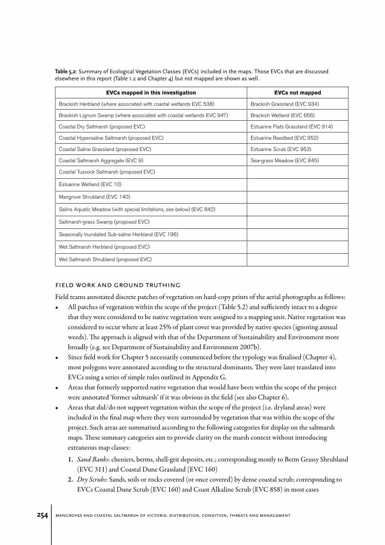
Table5.2: Summary of Ecological Vegetation Classes (EVCs) included in the maps. Those EVCs that are discussed elsewhere in this report (Table 1.2 and Chapter 4) but not mapped are shown as well.

EVCs mapped in this investigation EVCs not mapped

Brackish Herbland (where associated with coastal wetlands EVC 538) Brackish Grassland (EVC 934)

Brackish Lignum Swamp (where associated with coastal wetlands EVC 947) Brackish Wetland (EVC 656)

Coastal Dry Saltmarsh (proposed EVC) Estuarine Flats Grassland (EVC 914)

Coastal Hypersaline Saltmarsh (proposed EVC) Estuarine Reedbed (EVC 952)

Coastal Saline Grassland (proposed EVC) Estuarine Scrub (EVC 953)

Coastal Saltmarsh Aggregate (EVC 9) Sea-grass Meadow (EVC 845)

Coastal Tussock Saltmarsh (proposed EVC)

Estuarine Wetland (EVC 10)

Mangrove Shrubland (EVC 140)

Saline Aquatic Meadow (with special limitations, see below) (EVC 842)

Saltmarsh-grass Swamp (proposed EVC)

Seasonally Inundated Sub-saline Herbland (EVC 196)

Wet Saltmarsh Herbland (proposed EVC)

Wet Saltmarsh Shrubland (proposed EVC)

field work and ground truthing

Field teams annotated discrete patches of vegetation on hard-copy prints of the aerial photographs as follows:• All patches of vegetation within the scope of the project (Table 5.2) and sufficiently intact to a degree

that they were considered to be native vegetation were assigned to a mapping unit. Native vegetation was considered to occur where at least 25% of plant cover was provided by native species (ignoring annual weeds). The approach is aligned with that of the Department of Sustainability and Environment more broadly (e.g. see Department of Sustainability and Environment 2007b).

• Since field work for Chapter 5 necessarily commenced before the typology was finalised (Chapter 4), most polygons were annotated according to the structural dominants. They were later translated into EVCs using a series of simple rules outlined in Appendix G.

• Areas that formerly supported native vegetation that would have been within the scope of the project were annotated ‘former saltmarsh’ if it was obvious in the field (see also Chapter 6).

• Areas that did/do not support vegetation within the scope of the project (i.e. dryland areas) were included in the final map where they were surrounded by vegetation that was within the scope of the project. Such areas are summarised according to the following categories for display on the saltmarsh maps. These summary categories aim to provide clarity on the marsh context without introducing extraneous map classes:

1. SandBanks: cheniers, berms, shell-grit deposits, etc.; corresponding mostly to Berm Grassy Shrubland (EVC 311) and Coastal Dune Grassland (EVC 160)

2. DryScrubs: Sands, soils or rocks covered (or once covered) by dense coastal scrub; corresponding to EVCs Coastal Dune Scrub (EVC 160) and Coast Alkaline Scrub (EVC 858) in most cases


3. EstuarineScrub: Wetland Melaleuca scrubs; almost always corresponding to the EVC Estuarine Scrub (EVC 953)

4. Woodlands: Areas covered (or formerly covered) by Eucalypt-, Banksia- or Sheoak-dominated vegetation; corresponding to many different EVCs, often including Damp Sands Herb-rich Woodland (EVC 3) or Heathy Woodland (EVC 48)

5. Wetlands: Areas covered with tall monocots (grasses or graminoids); almost always corresponding to the EVC Estuarine Reedbed, but occasionally other EVCs

6. Grassland: Areas covered (or once covered) with largely-treeless grasslands, usually of Poa spp.; almost always corresponding to Estuarine Flats Grassland (EVC 914)

7. Spoil: Artificial material covering former saltmarsh.

Some patches of native vegetation did not readily fit into one of the mapping units described above. These areas were described as follows:• Mosaics. Mosaics are areas in which two or more discrete types of vegetation are so intricately patterned

that their boundaries could not be mapped at the given scale of 1:10,000. To maximise clarity of the resultant maps, we limited mosaics to two units only. Where more than two saltmarsh units were apparent during the field inspections, we used the ‘CoastalSaltmarsh (Aggregate)’ unit as described below.

• CoastalSaltmarsh (Aggregate). This unit was used for areas that were too complex to describe in any other way. They generally contained elements of three or more saltmarsh units in mosaic.

• CoastalSaltmarsh (Unknown). This unit was used to describe areas to which access could not be gained during field work, and for which the phototype was ambiguous (see below). As described in the GIS metadata, this unit is encoded along with Coastal Saltmarsh Aggregate, above, but is recognisable by the recorded lack of ground-validation.

Mapping the EVC Saline Aquatic Meadow (EVC 842) was particularly difficult. Ephemeral pools and apparently unvegetated areas associated with coastal saltmarsh and mangroves are subject to significant temporal variation. They may on occasion be bare ground (empty pools), covered by open water, and/or they may support Saline Aquatic Meadow. In cases where we had no other specific information to guide us, we used the following mapping rules on the GIS:• Areas of bare ground and/or water (excluding artificial ponds, see below) totally surrounded by any of the

Saltmarsh units or Estuarine Wetland (EVC 10) are mapped as ‘Saline Aquatic Meadow/Bare Ground mosaic’. Those areas are assumed to be ephemeral brine pools that would sometimes support Saline Aquatic Meadow. We acknowledge that on rare occasions other EVCs may occupy areas of bare ground in this context (e.g. Brackish Aquatic Herbland (EVC 537), Sea-grass Meadow (EVC 845), Seasonally Inundated Sub-saline Herbland (EVC 196), or some of the Saltmarsh units with low absolute cover).

• Areas of bare ground and/or open water that are inliers between saltmarsh and mangroves are mapped as ‘Open Water/Bare Ground mosaic’. These areas are assumed to be open mudflats that do not trap water and become hypersaline.

• Areas of bare ground or open water within artificial ponds (e.g. saltworks) are mapped as ‘Open Water/Bare Ground mosaic’.

We acknowledge that bodies of water not enclosed by our map units may sometimes support Saline Aquatic Meadow. In larger saline water bodies (e.g. Lake Reeve when inundated), only portions might support this


EVC at any one time (presumably depeneding locally on depth, salinity and wave action). We did not attempt to map all occurrences of Saline Aquatic Meadow in Victoria, and no area statements are provided for this EVC.

Most patches of saltmarsh on publicly accessible land (e.g. Crown land, parks, municipal reserves, land managed by Melbourne Water or Parks Victoria, etc.) were visited for ground truthing. In some cases, it was adequate for the purposes of mapping and inventory to view the saltmarsh with binoculars. On-ground inspections of other areas, however, required access through or to private land. In these cases permission was sought where contact could be made readily with the landholder. Access to or through private land was required for Belfast Lough (Port Fairy), Fitzroy River, Lake Yambuk, Gellibrand River, Aire River, Phillip Island, Shallow Inlet, the western coast of Port Phillip and many portions of the Gippsland Lakes.

Where channels or inaccessible private land prevented foot or vehicle access, areas were visited by kayak or boat. Examples of areas visited in this way include the Gellibrand River, Aire River, Bass River and Anderson Inlet.

For the purposes of dividing the teams’ labour resources, each team was assigned to a different part of the coast for survey. Table 5.3 summarises the division of the field survey and the survey effort for each area. Note that survey effort was generally more intensive in very complex areas of saltmarsh (compare the more complex Port Phillip Bay with the relatively simple but extensive marshes of Western Port).

Table5.3: Regional effort in surveying areas across the Victorian coastline. The Arthur Rylah Institute has been abbreviated to ARI. Figures represent actual days spent in the field, regardless of how many people constituted a field team.

Area Team Survey effort (approx. days)

South Australia border to Breamlea ARI 27

Breamlea to Melbourne Biosis Research 80

Melbourne to Walkerville ARI 17

Walkerville to Golden Point (i.e. central Gippsland Lakes)

Ecology Australia 48

Golden Point to NSW border Biosis Research 40

Despite the effort put into ground truthing, many parts of the coast with mangrove or coastal saltmarsh could not practically be visited or directly observed given the time constraints of this project, even with the aid of binoculars or kayak (e.g. areas east of Mallacoota Inlet, sections of the northern French Island coast, islands in the Nooramunga area, and many small portions of land elsewhere along the coast). These areas were assigned an EVC (although generally not a structural dominant) based solely on aerial photograph interpretation, using knowledge about phototypes (i.e. the appearance of an area in an aerial photograph) gained from nearby field work. As described in the GIS metadata (Appendix H), all saltmarsh patches that were not directly observed are clearly flagged in the map dataset.

In total, we mapped approximately 70% of vegetation (by area) by direct observation of the polygon, either on foot, by kayak or more remotely by binoculars. That figure excludes inliers of non-saltmarsh vegetation, along with bare ground. Given the size and length of some polygons, the accuracy of the estimate is rounded to the nearest 5%.


map preparation

The distribution of coastal saltmarsh is represented in the final digital map dataset as a series of spatially referenced polygons. All polygons were constructed ‘by hand’ using Arcview 3.2 (ESRI), traced directly from aerial photographs as annotated by the ground-truthing teams. To permit fluid boundaries on the shapes and to lessen the burden of ‘mouse-clicking’ in their construction, a stream digitiser was used with a sensitive screen and stylus (Minnesota Department of Natural Resources 2000; using a Wacom tablet screen). This instrumentation allowed direct tracing of the shapes on the screen in the same manner as has been used traditionally with a pencil and tracing paper over an annotated map image. The polygons were attributed with a series of fields describing their vegetation type, etc. The complete GIS metadata are included in Appendix H. Examples of the maps are shown below, digital images of all maps are provided on the accompanying CD (‘Mangroves and coastal saltmarsh of Victoria: mapping outputs’). The complete GIS map files are held by the Department of Sustainability and Environment.

As discussed above, map scale is an important issue that must be practically resolved when creating a vegetation map. The topic is especially problematic with coastal saltmarsh as the vegetation is often patterned at a very fine scale and there is almost no limit to how finely its patterning could be recorded. We selected our scale of presentation (display at 1:5,000) using mundane but common considerations outlined by Meentemeyer (1989): i) the grain size of the aerial photograph templates (0.15 m to 1.25 m); ii) scale at which decisions are made (~property scale); iii) the standards set by previous maps (often 1:25,000); iv) the types of software commonly available to users; v) the scope of the project; and vi) the resources (especially funds) available. Another consideration was the experience and intuition of the field team in deciding what level of patterning was meaningful in describing the vegetation. Notwithstanding these complications, there is no doubt that the maps produced are fit for their purpose and far better than previously existing resources (cf. summary of prior mapping activities: see Chapter 1.15).

Since we employed multiple field teams for the ground-truthing component of the project (Table 5.3), it was particularly important to define the scope and constraints of the map scale clearly so that all teams were able to map in a consistent way. To this end, it was agreed that all features with a diameter of less than 20 m or an area of less than 0.04 ha were omitted from the spatial dataset, but linear features less than 20 m wide could be shown if they covered an extensive area (> 100 m long) or were part of a larger patch (e.g. if they formed an ‘isthmus’ of vegetation joining two large patches).

The stream digitiser allows the user to set the distance between vertices, so that the fluid line created by the tool is in fact a series of small straight lines of a set minimum length. The approach allows the resolution of polygon boundaries to be standardised, such that inappropriately high magnification of the maps – that is a magnification beyond their intended level of resolution – leads to the appearance of jagged edges in the viewed image. We set the inter-vertex distance at 5 m.


5.3 Mappingandinventory–summaryofresults

examples of mapping outputs

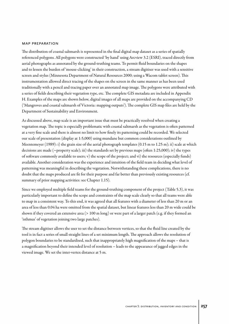
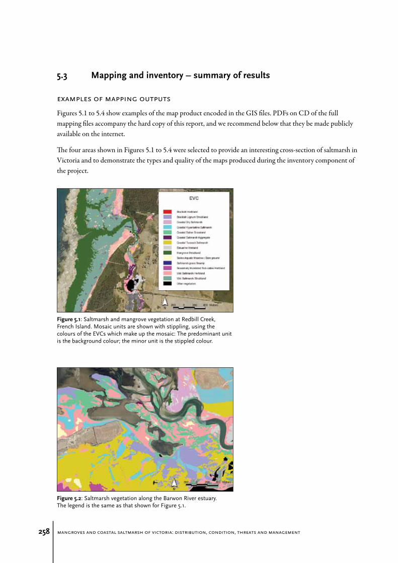
Figures 5.1 to 5.4 show examples of the map product encoded in the GIS files. PDFs on CD of the full mapping files accompany the hard copy of this report, and we recommend below that they be made publicly available on the internet.

The four areas shown in Figures 5.1 to 5.4 were selected to provide an interesting cross-section of saltmarsh in Victoria and to demonstrate the types and quality of the maps produced during the inventory component of the project.

Figure5.1: Saltmarsh and mangrove vegetation at Redbill Creek, French Island. Mosaic units are shown with stippling, using the colours of the EVCs which make up the mosaic: The predominant unit is the background colour; the minor unit is the stippled colour.

Figure5.2: Saltmarsh vegetation along the Barwon River estuary. The legend is the same as that shown for Figure 5.1.


Figure5.3: Mangrove and saltmarsh vegetation at Rhyll Inlet, Phillip Island. The legend is the same as that shown for Figure 5.1.

Figure5.4: Saltmarsh vegetation at Lake Reeve, Gippsland. The legend is the same as that shown for Figure 5.1.

The use of EVCs nested within the previously-used aggregate unit allows a great deal of information to be revealed that was previously hidden. In fact, one of the strengths of our mapping is that it provides sufficient detail to reveal the spatial manifestation of ecological processes within saltmarsh. Often the causes of these patterns are obscure, in which case the mapping helps us form hypotheses as to the causes. For example, given that Estuarine Wetland (EVC 10) commonly occurs where saline conditions are relieved by periodic freshwater flows, the occurrence of this EVC in the upper reaches of Redbill Creek inland from the saltmarsh (Figure 5.1), on the lower Barwon River estuary near only the main stream channel (Figure 5.2), and its almost total absence from Rhyll Inlet (Figure 5.3) together suggest that these three coastal systems have very different freshwater inputs. On the basis of the mapping, it would seem that Rhyll Inlet receives no appreciable freshwater inflow, that Redbill Creek receives modest flows that do not flush the lower marsh, and that the main channel of the Barwon River receives freshwater flows that penetrate to the mouth, but do not often flood the saltmarsh which is distant from the main channel. Detailed on-ground observations could readily test such proposals.


statewide inventory

The high resolution of the mapping allows us to prepare inventory information about saltmarsh and mangrove distributions that is far more accurate than previously possible. As outlined in Chapter 1, current estimates of the area of mangroves and coastal saltmarsh in Victoria, if available at all, vary over a two-fold range.

The mapping indicates that Victoria contains 19,212 ha (~192 km2) of Coastal Saltmarsh Aggregate (see Chapter 4); 5,177 ha (~52 km2) of mangroves (EVC 140); and 3,227 ha (~32 km2) of Estuarine Wetland (EVC 10). These figures exclude some EVCs that may occasionally be considered saltmarsh on less spatially-resolved maps, such as Seasonally Inundated Sub-saline Herbland (EVC 196, approximately 647 ha) and Saline Aquatic Meadow (EVC 842, no area calculated since it is an ephemeral EVC). For the purposes of calculation, when EVCs occur in mosaic we assumed that each member of the mosaic made up half the area. Notwithstanding this assumption and the unavoidable constraints imposed by map scale, our estimate is by far the most accurate to date.

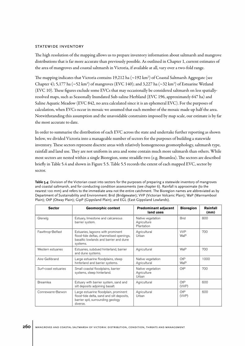
In order to summarise the distribution of each EVC across the state and undertake further reporting as shown below, we divided Victoria into a manageable number of sectors for the purposes of building a statewide inventory. These sectors represent discrete areas with relatively homogeneous geomorphology, saltmarsh type, rainfall and land use. They are not uniform in area and some contain much more saltmarsh than others. While most sectors are nested within a single Bioregion, some straddle two (e.g. Breamlea). The sectors are described briefly in Table 5.4 and shown in Figure 5.5. Table 5.5 records the extent of each mapped EVC, sector by sector.

Table5.4: Division of the Victorian coast into sectors for the purposes of preparing a statewide inventory of mangroves and coastal saltmarsh, and for conducting condition assessments (see chapter 6). Rainfall is approximate (to the nearest 100 mm) and refers to the immediate area not the entire catchment. The Bioregion names are abbreviated as by Department of Sustainability and Environment: Brid (Bridgewater); VVP (Victorian Volcanic Plain); WaP (Warrnambool Plain); OtP (Otway Plain); GipP (Gippsland Plain); and EGL (East Gippsland Lowlands).

Sector Geomorphic context Predominant adjacent land uses

Bioregion Rainfall(mm)

Glenelg Estuary, limestone and calcareous barrier system.

Native vegetationAgriculturePlantation

Brid 800

Fawthrop-Belfast Estuaries, lagoons with prominent flood-tide deltas, channelised openings, basaltic lowlands and barrier and dune systems.

AgriculturalUrban

VVPWaP

700

Western estuaries Estuaries, subdued hinterland, barrier and dune systems.

Agricultural WaP 700

Aire-Gellibrand Large estuarine floodplains, steep hinterland and barrier systems.

Native vegetationAgricultural

OtP WaP

1000

Surf-coast estuaries Small coastal floodplains, barrier systems, steep hinterland.

Native vegetationAgricultureUrban

OtP 700

Breamlea Estuary with barrier system, sand and silt deposits adjoining basalt.

Agricultural OtP(VVP)

600

Connewarre-Barwon Large estuarine floodplain, prominent flood-tide delta, sand and silt deposits, barrier spit, surrounding geology diverse.

AgriculturalUrban

OtP(VVP)

600


Sector Geomorphic context Predominant adjacent land uses

Bioregion Rainfall(mm)

Londsdale lakes Saline lakes isolated from ocean by complex sand and silt deposits, limestone.

Agricultural Urban

OtP 700

Salt Lagoon Saline lake isolated from the ocean. Agricultural Urban

OtP 700

Swan Bay Embayment, sheltered by series of sand spits.

Agricultural Urban

OtP 700

Mud Islands Sand and shell-grit shoals, anchored on calcarenite.

None / Ocean Native vegetation

NA 700

Port Phillip Coast of large embayment, largely low-relief basaltic hinterland.

Water treatmentAgricultural UrbanIndustrial

VVPOtP

600

The Inlets Partly channelised outflow of drained swamp, tidal channels from sheltered coast of embayment

Agricultural GipP 800

Western Port Low-energy coast of large embayment, minor estuaries, large tidal range, extensive mudflats.

Agricultural Native vegetationUrban

GipP 800

French Island Coast of large island within Western Port, mostly sandy deposits, large tidal range.


GipP 800

Rhyll Inlet Sheltered embayment behind sand spit. UrbanAgricultural

GipP 800

Lang Lang coast Cliffed and eroding coast. Agricultural GipP 800

Bass River Large floodplain on Western Port coast. Agricultural GipP 800

Powlett-Kilcunda Small estuaries. Agricultural GipP 800

Anderson Inlet Shallow, sheltered inlet behind barrier, estuarine input.

AgriculturalNative vegetationUrban

GipP 800

Shallow Inlet Shallow, sheltered tidal inlet behind barrier.


Wilsons Promontory Sheltered portions of coast. Native vegetation WPro 900

Corner Inlet Sheltered coast, geology various, minor estuaries, extensive sandflats and mudflats.


GipP 900

Nooramunga coast Sheltered coast opposite Nooramunga Islands, geology various, minor estuaries, extensive sandflats and mudflats.


GipP 800

Nooramunga islands Complex of quartz sand barrier deposits forming sheltered inlets, extensive sandflats and mudflats.


GipP 800

Jack Smith Lake Lake separated from ocean by sand barrier.


Lake Reeve Saline lake system separated from ocean by sand barriers. Bordered by complex system of contraction ridges.

Native vegetationAgriculturalUrban

GipP 700

Lake Wellington Coastal Lagoon separated from ocean by large sand barriers.

AgriculturalNative vegetation

GipP 700

Lakes Victoria and King

Coastal Lagoons separated from ocean by large sand barriers.


GipP 700

East Gippsland inlets Inlets, barrier-built lagoons and estuaries.

Native vegetation EGL 900


Figure5.5: Locations of the sectors described in Table 5.4. A) shows the western coast of the state; B) the eastern coast. A few very small areas of saltmarsh are not visible at this scale, and are included with the nearest sector (e.g. Balcombe Creek is within Port Phillip).


Sec

tor

WS

HW

SS

CTS

CD

SC

HS

CS

GS

GS

CS

All

salt

mar

shE

WM

SS

ISH

Aire

-Gel

libra

nd0

00

00

00

00

22

10

0

And

erso

n In

let

58

26

72<

10

16

10

33

349

81

15

80

Bas

s R

iver

7575

33

00

0<

115

7<

11

50

Bre

amle

a9

687

59

35

50

40

033

18

0<

1

Con

new

arre

-Bar

won

702

10

44

48

711

739

43

10

1605

13

34

98

4

Cor

ner

Inle

t1

81

18

32

5<

10

10

48

437

13

84

60

Eas

t Gip

psla

nd in

lets

15

80

15

70

< 1

05

523

570

20

0

Faw

thro

p-B

elfa

st5

4<

1<

10

03

00

574

00

Fren

ch Is

land

26

64

876

780

30

20

860

26

475

0

Gle

nelg

Riv

er8

01

00

00

00

183

40

0

Jack

Sm

ith L

ake

781

02

572

70

70

16

312

3571

01

68

Lake

Ree

ve67

60

51

34

85

11

51

20

39

321

946

40

30

1

Lake

Wel

lingt

on2

12

30

52

14

01

23

60

36

2399

41

30

13

Lake

s Vi

ctor

ia a

nd

Kin

g1

31

80

28

41

94

80

59

1836

62

20

79

Lang

Lan

g co

ast

80

< 1

00

00

210

18

20

Lond

sdal

e la

kes

471

45

31

82

00

125

80

2

Mud

Isla

nds

16

18

< 1

00

00

034

00

0

Noo

ram

unga

coa

st70

98

572

48

29

01

20

10

519

601

21

99

40

Noo

ram

unga

isla

nds

572

59

86

23

14

00

01

19

1926

34

12

470

Por

t Phi

llip

172

20

26

22

60

38

31

60

28

313

781

26

< 1

Pow

lett

-Kilc

unda

16

03

00

00

019

52

00

Rhy

ll In

let

17

726

60

00

210

3<

19

30

Sal

t Lag

oon

90

14

< 1

10

00

033

< 1

0<

1

Sha

llow

Inle

t79

711

8<

10

< 1

03

171

80

0

Sur

f-co

ast e

stua

ries

40

30

00

00

71

70

0

Sw

an B

ay5

81

86

69

08

00

90

411

60

0

The

Inle

ts9

20

13

00

00

749

68

0

Wes

tern

Por

t1

82

761

39

80

00

98

1088

58

12

30

0

Wes

tern

est

uarie

s3

70

00

02

40

061

49

00

0

Wils

ons

Pro

mon

tory

81

40

2<

10

00

< 1

123

55

40

Tota

l85

1238

0126

4115

8376

338

33

1526

1921

232

2751

7764

7

Table5.5: The extent (hectares) of coastal marsh EVCs across Victoria in each of the sectors described in Table 5.4. The sectors are arranged west-east (approximately) and area values are expressed to the nearest hectare. The abbreviations are as follows: CS (Coastal Saltmarsh Aggregate), WSH (Wet Saltmarsh Herbland), WSS (Wet Saltmarsh Shrubland), CTS (Coastal Tussock Saltmarsh), CSG (Coastal Saline Grassland), SGS (Saltmarsh-grass Swamp), CDS (Coastal Dry Saltmarsh), CHS (Coastal Hypersaline Shrubland), EW (Estuarine Wetland), MS (Mangrove Shrubland), SISH (Seasonally-inundated Sub-saline Herbland). Saline Aquatic Meadow, Brackish Lignum Swamp and Brackish Herbland are not included in this tally, because we did not map all of these EVCs across the state, as described above. Note that due to the inclusion of the ‘unresolved’ aggregate unit which includes unknown areas of other saltmarsh EVCs, the areas given for WSH, WSS, CTS, SGS, CDS and CHS are minimum values.


5.4 Currentecologicalcondition

‘ecological condition’ in the victorian context

As outlined in Appendix A, the project team was charged with developing ‘…amethodforassessingtheconditionofintertidalecosystems,consistentwithbutbuildingonthetechniquesoutlinedinVictoria’sVegetationFrameworkandIndexofWetlandCondition…’ and assessing the condition of coastal saltmarsh and mangroves ‘…atascalethatwillguideandinformbothregionalplanningprocessesandinvestmentprioritization’. We interpreted this requirement as incorporating two distinct tasks: • Task 1: provide an overview of the current ecological condition of coastal saltmarsh in Victoria, suitable

for regional planning and investment processes.• Task 2: devise a detailed condition-assessment method suitable for application by land managers and

planners, which was able to detect finer-scale patterns of ecological condition and to be used beyond the life of this project.

As described in Chapter 1.14, there is no universally accepted concept of ecological ‘condition’, despite the fact that the term is widely used and is understood in some way by a wide audience (Gibbons & Freudenberger 2006; Parkes & Lyon 2006). In order to meet the expectations of the project brief, we must nevertheless settle on a definition that is practical and practicable. A small number of protocols have been developed elsewhere in Australia to indicate ecological condition (see Chapter 1.14), but none are suitable for our purposes.

We take our cue from current Victorian usage to refine an appropriate definition of condition. Victoria’sVegetationFramework:AFrameworkforAction (Department of Sustainability and Environment 2002b; i.e. the ‘Habitat Hectares’ approach as outlined in Parkes et al. 2003 and Department of Sustainability and Environment 2004b) does not explicitly define ecological condition, and the definition provided for the Index of Wetland Condition (Department of Sustainability and Environment 2005b, page I; see also Department of Sustainability and Environment 2006, 2007a, 2009b) is not one that could be easily implemented in the field (see Chapter 1.14). Neverthless, a view of condition is implicit in both approaches and it seems that ecological ‘condition’ is essentially synonymous with ecological ‘quality’. We use the term ‘ecological condition’ in the following senses:• Ecological condition measures the retention or loss of those ecological attributes that characterise an

ecosystem in its desired state.• The desired state is the state of that system when natural ecological and geomorphological processes are

able to operate (this is often equivalent to the ‘mature and long-undisturbed’ state described for Habitat Hectares and the Index of Wetland Condition). Such a state is often assumed to be one which is most self-sustaining and resilient in the face of disturbance, spatially unfragmented given the site in question, able to support maximally-complex ecological structures and networks, able to support maximal biodiversity given the systemic constraints on production, and one which poses minimum threat to other ecological systems.

• The desired state is described by a ‘benchmark’ against which individual sites are assessed. The difference between a given site and the benchmark is assessed using measurable ‘indicators’, which are assumed to provide an ecological summary of ecological condition.


The assumptions within this view and some of the practical consequences of its use are best made explicit. First, the concept is inherently and unapologetically comparative, anthropocentric and subjective (Parkes & Lyon 2006). Second, it has been selected from many possible ideas of ‘ecological condition’, because we believe it is most appropriate for use in the current context.

Third, the use of benchmarks permits the comparison of one system with another; in contrast, the use of raw measures generally does not without further interpretation. Fourth, benchmarks must be compiled in order to assess condition. That activity requires interpretation, analysis and extrapolation, and is subject to error (McCarthy et al. 2004; Parkes & Lyon 2006).

Fifth, there is an unclear relationship between systems which are ‘long undisturbed’ (see Habitat Hectares) and those in which ‘natural ecological processes operate’ (see our definition above). The assumption that a lack of disturbance is correlated with the maintenance of natural processes, greater diversity and greater stability or resilience is not always true (see McCann 2000; Folke et al. 2004; Ives & Carpenter 2007).

Sixth, such a view of condition deals poorly with natural seral or cyclical ecological changes. Distinguishing changes that represent normal fluctuations from those we wish to recognise as representing a loss of condition is difficult (McCarthy et al. 2004).

Seventh, it is often unclear whether the view of ecological condition refers only to the present (a ‘snapshot’), or whether it considers site history or prognosis. Many value judgements about current ecological condition are based on an (incomplete) understanding of likely consequences. The demarcation between assessing the present and the future is rarely simple. The corollary is that multiple assessments are required to determine whether a site is improving or declining in condition.

Finally, the indicators used for defining a benchmark and assessing condition may not necessarily be the best guide to overall ecological condition as described above.

Although our definition of condition given above refers broadly to ecological processes, both the Index of Wetland Condition and Habitat Hectares approaches have a strong focus on vegetation. Observable vegetation attributes are assumed to provide a summary of ecological processes that are not measured (e.g. see Niemi & McDonald 2004; Gibbons & Freudenberger 2006). Given the difficulty involved for the non-specialist in using many other potential indicators (e.g. measuring productivity, invertebrate diversity, etc.), vegetation is probably the most practical and efficient indicator of general saltmarsh condition. Our condition metric, described below, therefore has an explicit focus on vegetation.

In some contexts ecological condition is not assessed directly at all, but is replaced by the observation of ‘threats’, ‘degrading processes’ or their impacts (whether past, active or potential). Such a shift is appropriate in situations where it is known that a particular action or process has detrimental effects on a given system, but the effects themselves are much more difficult to measure than the threatening process are to identify. The Index of Wetland Condition, for example, uses ‘threat measures’ as part of its condition assessment (Department of Sustainability and Environment 2005b, 2009b; see also Chapter 1.14). That approach may be appropriate when the purpose of assessment is to rank actions and manage individual threats: if an ongoing threat is the thing that will be managed, it is sensible to measure it and assume that its magnitude and occurrence are somehow related to ecological condition. Our assessment of saltmarsh condition across the state takes the approach of assessing the occurrence of degrading processes.


task 1: overview of ecological condition of mangroves and coastal saltmarsh and assessment of threats in victoria

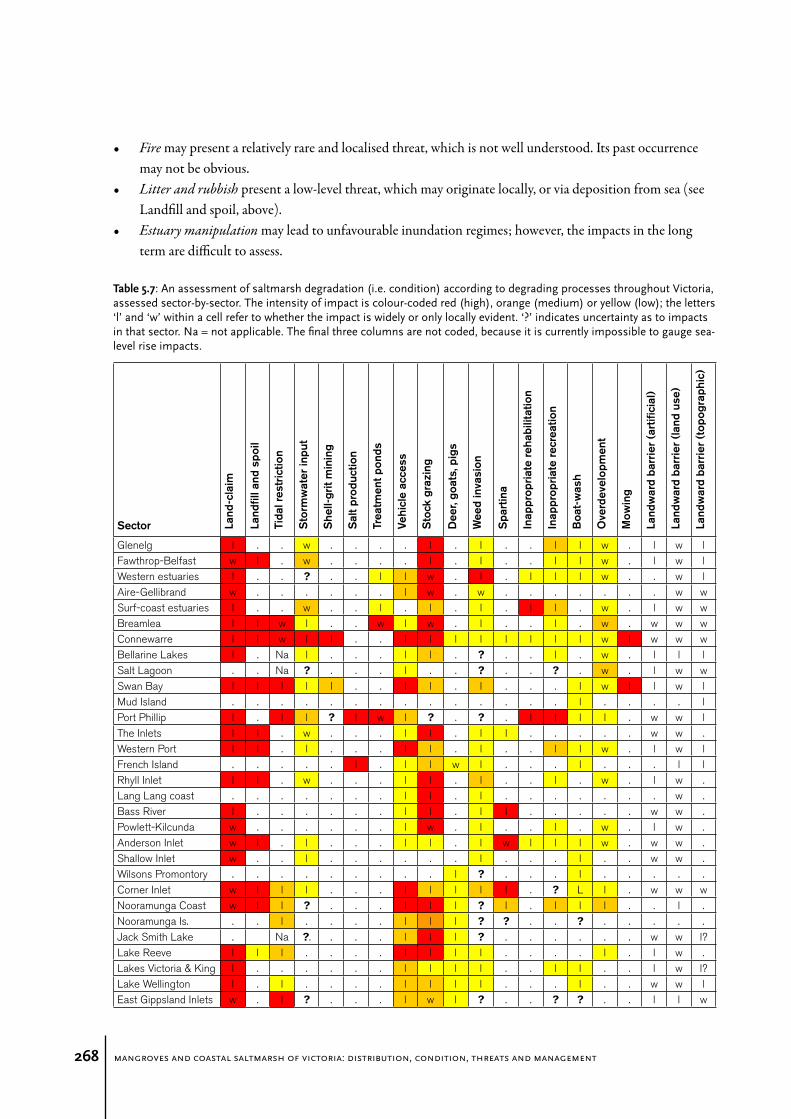
For each sector of the coast (see Table 5.4 and Figure 5.5), we assessed current saltmarsh condition with a subjective assessment of how severe the impacts of various degrading processes have been to date. Table 5.6 describes the threatening processes, and Table 5.7 presents the results of the assessment on a sector-by-sector analysis of the Victorian coast. Note that many of the processes are described in greater detail in the literature review (Chapters 1.11–1.13) and their specific application shown in the management template developed for the Barwon River estuary (Chapter 7). Impacts on estuarine systems other than saltmarshes and mangroves were not addressed, nor did we consider ecological changes which may have lead to expansion in the area or extent of coastal saltmarsh.

The intensity of impact was scored using the following simple categories:• H: high: Saltmarsh largely destroyed or lost, massive visual and ecological impact• M: medium: Saltmarsh visibly structurally modified and of reduced biological diversity.• L: low: detrimental impact discernable with close inspection or measurement, but marsh essentially

intact.

Each of these categories was further annotated as to how widely the impact had been felt:• w: widely within the sector (affecting > ~5% of original marsh area)• l: locally in relatively small, localised places (< ~5% of original marsh area).

We also assessed the likely landward barriers to saltmarsh migration under changes to sea levels as being widespread, localised, or absent in that part of the coast.

We undertook the assessment in two ways. The first was an inspection of aerial photographs for evidence of levees, drains etc. The second was from the assessment sheets completed during field work which noted the relevant threats. Given that we had little spatially explicit data on EVCs at the commencement of the project to produce a stratification and the difficulties of remote site access, these assessments were done opportunistically. Sites were selected which typified an area (in the opinion of the field worker), or which were unusual in some way (due to a particular threat, management history, etc.). Each assessment referred to a site 50 m in radius. Given their method of selection, the information gathered is strongly biased, but provides a good coverage of the range of site attributes.

The intensity of impact was not adjusted for the context or size of each sector: a ‘high’ impact is a high impact if it meets the description above. Some degrading processes are always ranked high as threatening processes (e.g. land-claim), whereas others may occur with different degrees of severity (e.g. weed invasion, damage by stock, vehicle damage, etc.). The extent of impact is relative to the size of the sector: a local impact on the Western Port coastline may be larger in extent than a widespread impact on the Fawthrop Lagoon.

The likely future impact from each degrading process has not been scored sector-by-sector, partly because the future is inherently unpredictable and partly because the future impact is possibly more dependent on the type of the threat than the locality. We note the likely future impact of each threat below (Table 5.5), but caution that these predictions are the subjective judgement of the project team and may be subject to unforeseeable changes.


Table5.6: Description of threatening processes likely to affect mangroves and coastal saltmarsh in Victoria.

Degrading process Definition Future direction

Land-claim Total destruction through engineering works (e.g. drains, levees) (often referred to as ‘reclamation’, a term we deliberately avoid).

Diminishing

Landfill and spoil Dumping of large quantities of material including soil onto the marsh surface, burying it.

Unknown

Tidal restriction Retardation of normal inundation through engineering works, not including those covered above (e.g. culverts).

Probably diminishing

Stormwater input Introduction of waste water, altering salinity and flooding regime and sometimes introducing pollutants.

Unknown

Eutrophication Enrichment with plant nutrients that results in increased primary production or biomass accumulation.

Probably increasing

Shell-grit mining Removal of shell-bank material causing soil disturbance and changed inundation patterns.

Diminishing

Salt production Creation of saline evaporation ponds for salt production using engineering works.

Diminishing

Treatment ponds Creation of ponds to receive and hold fresh water for purification or storage. Diminishing

Vehicle access Physical damage to soil and plants caused by vehicles or motorbikes. Probably increasing

Stock grazing Use of marsh as pasture causing damage to plants and soil (without reliance on drainage works, covered above).

Unknown

Deer, goats, pigs Browsing and trampling by deer, goats and pigs. Unknown

Weed Invasion Loss of native species by exotics (not including *Spartina spp). Increasing

*Spartina invasion Invasion and alteration of marsh dynamics by *Spartina. Increasing

Inappropriate rehabilitation

Ill-conceived construction of ‘wetlands’, deliberate planting of non-native species, or of inappropriate indigenous species.

Unknown

Inappropriate recreation

Physical damage to vegetation and soils due to human foot traffic, etc. Probably increasing

Boat-wash Erosion of marsh edges caused by boat-generated waves. Unknown

Mowing Mowing or slashing of saltmarsh. Unknown

Overdevelopment Construction of buildings near or on saltmarsh. The impact of this process is considered outside the marsh.

Probably increasing

Several important degrading processes have not been scored in Table 5.6, as discussed below. Their omission should not be taken to indicate any lack of importance:• Sea-levelrise is largely yet to manifest strongly, but will be ubiquitous across the Victorian coast, even if it

will be mediated by local factors that are virtually impossible to predict (see Chapter 6). Together these factors make it difficult to assess its current impact.

• Rabbits,haresandfoxesare considered near-ubiquitous, but have particularly significant impacts in areas of drier saltmarsh.

• Mangroveencroachment may threaten saltmarsh areas, but we do not have the data to assess the threat, particularly whether it is locally the result of human-induced changes or is an unavoidable natural change associated with land subsidence.

• Introducedinvertebratesmay present significant threats, but we do not have the data to allow a sector-by-sector assessment.


• Firemay present a relatively rare and localised threat, which is not well understood. Its past occurrence may not be obvious.

• Litterandrubbish present a low-level threat, which may originate locally, or via deposition from sea (see Landfill and spoil, above).

• Estuarymanipulation may lead to unfavourable inundation regimes; however, the impacts in the long term are difficult to assess.

Table5.7: An assessment of saltmarsh degradation (i.e. condition) according to degrading processes throughout Victoria, assessed sector-by-sector. The intensity of impact is colour-coded red (high), orange (medium) or yellow (low); the letters ‘l’ and ‘w’ within a cell refer to whether the impact is widely or only locally evident. ‘?’ indicates uncertainty as to impacts in that sector. Na = not applicable. The final three columns are not coded, because it is currently impossible to gauge sea-level rise impacts.

Sector Land

-cla

im

Land

fill a

nd s

poil

Tida

l res

tric

tion

Sto

rmw

ater

inpu

t

She

ll-gr

it m

inin

g

Sal

t pro

duct

ion

Trea

tmen

t pon

ds

Vehi

cle

acce

ss

Sto

ck g

razi

ng

Dee

r, go

ats,

pig

s

Wee

d in

vasi

on

Spa

rtin

a

Inap

prop

riate

reha

bilit

atio

n

Inap

prop

riate

recr

eatio

n

Boa

t-w

ash

Ove

rdev

elop

men

t

Mow

ing

Land

war

d ba

rrie

r (a

rtifi

cial

)

Land

war

d ba

rrie

r (la

nd u

se)

Land

war

d ba

rrie

r (t

opog

raph

ic)

Glenelg l . . w . . . . l . l . . l l w . l w lFawthrop-Belfast w l . w . . . . l . l . . l l w . l w lWestern estuaries l . . ? . . l l w . l . l l l w . . w lAire-Gellibrand w . . . . . . l w . w . . . . . . . w wSurf-coast estuaries l . . w . . l . l . l . l l . w . l w wBreamlea l l w l . . w l w . l . . l . w . w w wConnewarre l l w l l . . l l l l l l l l w l w w wBellarine Lakes l . Na l . . . l l . ? . . l . w . l l lSalt Lagoon . . Na ? . . . l . . ? . . ? . w . l w wSwan Bay l l l l l . . l l . l . . . l w l l w lMud Island . . . . . . . . . . . . . . l . . . . lPort Phillip l . l l ? l w l ? . ? . l l l l . w w lThe Inlets l l . w . . . l l . l l . . . . . w w .Western Port l l . l . . . l l . l . . l l w . l w lFrench Island . . . . . l . l l w l . . . l . . . l lRhyll Inlet l l . w . . . l l . l . . l . w . l w .Lang Lang coast . . . . . . . l l . l . . . . . . . w .Bass River l . . . . . . l l . l l . . . . . w w .Powlett-Kilcunda w . . . . . . l w . l . . l . w . l w .Anderson Inlet w l . l . . . l l . l w l l l w . w w .Shallow Inlet w . . l . . . . . . l . . . l . . w w .Wilsons Promontory . . . . . . . . . l ? . . . l . . . . .Corner Inlet w l l l . . . l l l l l . ? L l . w w wNooramunga Coast w l l ? . . . l l l ? l . l l l . . l .Nooramunga Is. . . l . . . . l l l ? ? . . ? . . . . .Jack Smith Lake . Na ?. . . . l l l ? . . . . . . w w l?Lake Reeve l l l . . . . l l l l . . . . l . l w .Lakes Victoria & King l . . . . . . l l l l . . l l . . l w l?Lake Wellington l . l . . . . l l l l . . . l . . w w lEast Gippsland Inlets w . l ? . . . l w l ? . . ? ? . . l l w


task 2: a detailed condition assessment method for coastal saltmarsh

TheVictoriancontext–existingmethodsforscoringecologicalcondition

In addition to assessing the action of degrading processes across the state, we were charged with the development of a condition metric that could be used to assess saltmarsh condition at a fine scale and was as consistent as possible with the existing Victorian approaches such as the Index of Wetland Condition and Habitat Hectares. This section presents a brief review of these two existing methods.

The two approaches share a number of aspirations and constraints, which our proposed method will also share. Those common aspirations and constraints identified below are largely paraphrased from the background report to the Index of Wetland Condition (Department of Sustainability and Environment 2006) and are the basis of the method developed below for these types of estuarine wetland:• It will be able to compare different wetlands.• It will be a tool for the surveillance of wetland extent and condition over a 10–20 year timeframe.• It will be suitable for use at a wetland at any time of year.• It will be designed to assess wetland condition in a single visit.• It will be a rapid assessment tool.• It will be simple, straightforward and inexpensive.• It will be able to be used by people with moderate ecological or botanical knowledge.• It will be easy to interpret.• Its form will be based on the most important ecological components of the wetland.• Its level of discrimination must be sufficient to determine significant human-induced change in the state

of the wetland.

Habitat Hectares

The Habitat Hectares approach was designed specifically to answer the needs of Victorian policy (Victoria’sNativeVegetationManagement:AFrameworkforAction, see Department of Sustainability and Environment 2002b). It is the only method endorsed for calculating vegetation offsets and for implementing other aspects of this policy. Habitat Hectares is a compound index made up of sub-indices which are combined and weighted to give an overall score (Parkes et al. 2003; Department of Sustainability and Environment 2004b). In addition to using the observed features of the site in question (e.g. vegetation structural diversity, tree size, presence of habitat elements such as logs, etc.), Habitat Hectares aims to assess how valuable a given site is in the broader context of fragmented habitat. To achieve this end, it penalise sites that are small and distant from other patches of native vegetation.

Habitat Hectares benchmarks currently exist for Mangrove Shrubland (EVC 140) and Coastal Saltmarsh (EVC Aggregate 9). It is thus possible to assess these systems already using the Habitat Hectares approach, and such assessments will remain necessary and unavoidable for statutory processes for the foreseeable future. It is, however, acknowledged that Habitat Hectares encounters problems in systems that are temporally dynamic and/or structurally very simple (Parkes et al. 2003). Saltmarsh and mangroves are both these things, indeed as are many other wetlands. Habitat Hectares often uses a generic (default) score for wetlands where they are unable to be reliably assessed but must be included in offset calculations. It represents a solution for strategic planning and policy purposes, but does not allow an actual assessment of wetland condition.


Index of Wetland Condition

The Index of Wetland Condition was designed to fill the gap noted above. It allows land managers (notably Catchment Management Authorities) to evaluate wetland condition across their estates and monitor overall condition over time. It does not formally relate to Victoria’sVegetationFramework:AFrameworkforAction. Because of the difficulties in directly measuring ecological processes, the Index of Wetland Condition uses instead a range of indirect indicators, including assessments of degrading processes. While the Habitat Hectares approach is routinely applied to arbitrary ‘zones’ (areas considered to have a homogeneous condition or state) the Index of Wetland Condition generally applies to entire but discrete wetlands. As for Habitat Hectares, the Index of Wetland Condition penalises sites that have been fragmented, but the rationale and scoring systems of the two assessment techniques are quite different.

Chapter 1.14 provided an overview of the application of the Index of Wetland Condition in Victoria. The most salient conclusion from the perspective of the current study is that the Index is not intended for application to wetlands that are hydrologically influenced by marine waters (Department of Sustainability and Environment 2005b, 2006, 2007a, 2009b); thus it is not suitable for assessing ecological condition in mangroves or coastal saltmarsh. Clearly, there remains a substantive gap in the tools available to assess the ecological condition of Victorian wetlands, with saltmarsh and mangroves missing out. That is the gap our recommended method aims to fill.

TailoringanewmethodforVictoriancoastalsaltmarsh

We have taken the principles of the Index of Wetland Condition and Habitat Hectares approaches to create a simple metric for assessing the ecological condition of mangroves and coastal saltmarsh. The method is described in the next section. Before it is described, several pertinent ecological considerations, particularly prominent in intertidal systems, must be addressed.

The first is the issue of ‘catchment’, a term emphasised in the Index of Wetland Condition. In many coastal wetlands the idea of a catchment is of little relevance, especially since most of the water which flows into the wetland system comes from the ocean and not from the hinterland. Although we acknowledge that some coastal marshes receive fresh water from nearby streams or from ground water, we have not included a measure of catchment condition as part of the assessment. Similarly, the issue of water quality, which is prominent in the Index of Wetland Condition (e.g. salinity, nutrients) is often impossible to assess for mangroves and coastal saltmarshes through any reference to what is visibly occurring in the surrounding area, given the overarching role played by tidal flushing in intertidal wetlands. Such an omission, however, should not be taken as construing that nutrient enrichment in particular is a threat not faced by many coastal wetlands (see review in Chapter 1.11).

The idea of ‘spatial context’ is emphasised in both the Index of Wetland Condition and Habitat Hectares. Both approaches assume that the system being assessed is (or should be) ‘ecologically linked’ to nearby systems. That, however, may not always be the case and saltmarsh may, in fact, be comparatively ‘unlinked’ to neighbouring patches of native vegetation or ‘habitat’, even under natural conditions. Any (presumed) isolation relates to the extreme ecological conditions in saltmarsh: most plant and many animal species which are important in mangroves or coastal saltmarsh do not occur in adjacent areas. Despite the upper levels of coastal saltmarsh being susceptible to invasion by a wide range of exotic plants (Chapters 1.5 and 1.11),


many invasive species from adjacent areas are not capable of invading coastal saltmarsh. Furthermore, most saltmarsh species naturally occur in small, isolated populations, and must disperse via long-distance means using sea currents or widely ranging animal vectors. For these reasons, we elected not to assess context as part of our condition assessment.

Spatial context is also related to the size of a wetland. Habitat Hectares penalises small and fragmented sites, and the Index of Wetland Condition penalises such sites according to their percentage loss in area. Given the problems associated with ‘context’ just noted, we follow the Index of Wetland Condition approach in the method proposed for mangroves and coastal saltmarsh. We assume that the extent of any given site does not reflect its condition in relation to other sites (saltmarshes may naturally be very small); but we penalise sites that have lost area over time. In other words, size is not part of the benchmark perse, but each site is benchmarked against its own former size. This approach assumes more ‘marsh is good’ and sets the year 1750 as an arbitrary benchmark of extent (see Chapter 6).

Changes over time take on more complex shades when it comes to coastal saltmarsh that is adventive. In this case the presence of saltmarsh represents the degradation of another system; an example is provided by the Gippsland Lakes (see Chapter 6.1). If ecological processes are so changed that one ecological system is replaced by another, it is difficult to know how we should value each system. There is no single solution to this problem, but it is important for a condition metric to focus clearly on what it is assessing: if saltmarsh is present, our metric will assess it according to the attributes we expect to see in saltmarsh, without regard to any former system which has been displaced. Any assessments of broader ecological values from a historical perspective are important, but must be considered outside the scope of our proposed metric.

The Index of Wetland Condition assesses and penalises human-induced hydrological changes. This weighting is appropriate where the item being assessed is awetland, as an individual asset. But our metric aims to assess saltmarsh as an ecological entity, not as a single site. We considered scoring changes to the physical form and hydrology of a saltmarsh by scoring the degree of drainage, and tidal restriction due to culverts or bunds. That approach, however, in turn raises several significant problems.

First, hydrological conditions in estuarine and inter-tidal wetlands are extraordinarily complex, and vary greatly among sites. It is difficult to equate the degree of ecological change with any simple measure based on the extent of engineering works (e.g. a single poorly designed culvert may do far more damage than a large pond, or not).

Second, if sea-level rise forces the migration of coastal wetland systems into their hinterland, good management may in fact entail engineering works to ensure that desired habitats are preserved or recreated elsewhere. Penalising all sites that are engineered may be counter-productive in such a context.

Third, saltmarsh vegetation may have reached a relatively stable equilibrium after accommodating hydrological changes imposed a long time ago. There may be no good ecological reason to penalise such sites.

We do not incorporate any measure of engineered hydrological change into an overall site condition score. We do, however, acknowledge the great importance of hydrological changes and that there are some contexts where it is reasonable to penalise sites on the basis of human-induced hydrological changes. Our solution is to record information about engineering works (as a mandatory field) on the score sheet, but to leave them unscored. Assessors may wish to assign some value to this information when analysing the data at a later stage.


In addition to such conceptual considerations and the pragmatic issues outlined at the beginning of the section, there are several more technical issues we addressed when adapting the style of thinking used in Index of Wetland Condition and Habitat Hectares approaches to saltmarsh assessment. They are outlined below:

• Benchmarks, like those of the Index of Wetland Condition, are explicitly written to avoid underscoring naturally simple or species-poor wetlands (e.g. the saltmarshes of far-western Victoria). That involves a trade-off: once-complex sites that have been simplified may not be penalised, and very rich or diverse sites are not rewarded.

• The assessment method may be applied to a discrete wetland (as in the Index of Wetland Condition) or a zone within a wetland, provided that the zone is in a homogeneous condition (as in Habitat Hectares).

• The score sheet records raw values as well as categories and includes a measure of observer uncertainty. Both the Index of Wetland Condition and Habitat Hectares assign scores for each component by filtering a raw estimate through a thresholded scoring matrix, which results in coarse categories. Unfortunately the raw estimate is often lost, which makes statistical analysis difficult, particularly as the categories are unevenly thresholded. Our score sheet asks assessors to record an interval (upper and lower bounds) which they are sure would include the true value. Although not used directly in the condition assessment method, these data are likely to be useful for future monitoring studies (e.g. see McCarthy et al. 2004). There is a large literature on the use of intervals for gauging uncertainty in estimated parameters, which is beyond the scope of this report (e.g. see Klayman et al. 2006).

• Our weed-scoring categories are more sensitive than those of the Index of Wetland Condition or Habitat Hectares. We consider weed cover to be one of the most reliable and useful indicators of vegetation condition; it need not be influenced by benchmarks, which allows meaningful comparisons to be made between sites, regions and EVCs. Given that the number of such reliable condition measures is limited, we have attempted to maximise the resolution of the weed score.

• The weed-threat level is not scored, only the cover of weeds. We have done this for three reasons: i) assessing threat level is conceptually inconsistent with the desire to record condition as a snapshot; ii) saltmarsh has few weeds, and most of our proposed EVCs are not prone to large-scale invasion by more than a handful of species. A two-dimensional scoring matrix (cover X threat) seems unnecessarily complex; and iii) threat scoring requires weeds to be well classified.

• Organic litter is not scored (as it is in Habitat Hectares), since the accumulation of organic litter in a coastal saltmarsh may be changed markedly from day to day by tidal action.

The net result of these considerations is a considerably simpler system than the Index of Wetland Condition or Habitat Hectares. Our approach is described next.

DescriptionoftheproposedmethodforVictoriancoastalsaltmarsh

This section briefly describes the proposed condition metric for coastal saltmarsh in Victoria and presents step-by-step guidelines as to how an assessment should proceed. It does not describe issues related to logistics, private property access, nor health and safety. This section could form the basis of a condition assessment manual, if the proposed method is adopted. A draft score sheet (Appendix I) and draft benchmarks (Appendix J) are provided for the following EVCs which were considered in this project, and which are not amenable to the Index of Wetland Condition or Habitat Hectares assessments:


• Wet Saltmarsh Herbland• Wet Saltmarsh Shrubland• Coastal Tussock Saltmarsh• Coastal Dry Saltmarsh• Coastal Hypersaline Shrubland• Coastal Saline Grassland• Saltmarsh-grass Swamp• Seasonally Inundated Sub-saline Herbland (EVC 196)• Mangrove Shrubland (EVC 140)

Step1:Confirm that the condition assessment method is appropriate to answer the problem at hand. The score sheet offers the following prompts:• Is this assessment for the state-, region- or catchment-wide evaluation of intertidal wetland condition; or

the comparison of one intertidal system with another? If so, us this assessment sheet.• Is this assessment for use in calculating offsets or implementing any aspect of Victoria’sVegetation

Framework:AFrameworkforAction? If so, use the Habitat Hectares condition assessment method (Department of Sustainability and Environment 2004b) with the DSE-endorsed Habitat Hectares benchmarks or default scores.

• Is this assessment for the monitoring of a single site over time where subtle changes must be detected? If so, consider designing a purpose-built detailed monitoring method.

Step2:Define the zone to which the assessment will apply and select a benchmark. Each assessment must apply to a zone with• A single EVC, and• A single condition state.

The Habitat Hectares manual (Department of Sustainability and Environment 2004b) provides some guidance for defining zones. If the zone must be a portion of saltmarsh that can only be practically mapped as a mosaic, separate scores for each EVC can be combined into a total score by weighting each score by the proportion of area that the EVC covers within the mosaic (as per Habitat Hectares: Department of Sustainability and Environment 2004b, p. 13; and the Index of Wetland Condition: Department of Sustainability and Environment 2009b, p 28.).

Step3:Record the spatial location of the zone(s). Ideally this should be a polygon captured in a GIS. Spatial accuracy is paramount if spatial and temporal change is to be assessed.

Step4: Assess the onsite attributes of the zone. The score sheet prompts the observer to estimate the cover of different groups of plants, according to their life forms. These values are recorded as raw estimates, and as an interval representing the upper and lower bounds considered plausible by the observer. The life-form categories are those described for Habitat Hectares (Department of Sustainability and Environment 2004b) unless described otherwise. Cover estimates should be made by imagining what portion of the zone is shaded by the group of plants in question: all parts of the plant are included (leaves, branches, etc.), but any spaces or holes are excluded. Cover may overlap between life-form classes, but not between plants within a class. The score sheet also asks the observer to assess the relative proportions of the marsh which have been affected by various detrimental impacts.


Step5: Assess the percentage loss of extent in the zone. Reference to pre-1750 mapping or field observations should be used to assess how much of the original area has been lost due to land-use change. Adventive saltmarsh which has increased in size (possibly by an infinite proportion) is scored as 100%. (Note that assessing the percentage reduction in marsh area for portions of a marsh, then totalling and weighting each score by its area, will give the same overall percentage reduction as scoring the entire marsh. Thus, the level of division into different EVCs or zones has no impact on this part of the score for a given marsh).

Step6: Apply the scoring. The scoring rules take the raw estimates from steps 4 and 5 to derive a total score (out of 100). When deciding whether the life-form groups meet the benchmark criteria, the threshold is that shown on the benchmark (there is no concept of ‘effectively absent’ or ‘substantially modified’ as in Habitat Hectares, and no need to calculate whether 50% of the benchmark cover is reached).

5.5 Distributionof*Spartina inVictoria

The ground-truthing component of the mapping and inventory studies offered a unique opportunity to record patches of *Spartina spp. across Victoria. All patches or plants we observed were recorded and mapped, including the approximate density of the patch. In addition to our own field observations, we used data generously contributed by Parks Victoria for Lake Connewarre and Anderson Inlet. The Parks Victoria data for Anderson Inlet was used as a preliminary indication and guide, and was modified following field work carried out by kayak. Importantly, we found that *Spartina was absent from the interior of the large islands in Anderson Inlet, a distribution which presumably reflects its inability to invade these areas. We found *Spartina in several EVCs, notably EVC 140 Mangrove Shrubland and EVC 10 Estuarine Wetland, but also in Wet Saltmarsh Herbland, Coastal Saline Grassland and marginally in Wet Saltmarsh Shrubland. The data on *Spartina distributions are presented on a separate GIS layer (Appendix H), and are shown on the map images on the accompanying CD. Figure 5.6 presents a summary of the distribution of *Spartina throughout Victoria. Note that we have not differentiated between the two species of *Spartina present in Victoria (see Chapter 1.12) and the mapping and inventory data refer to both species.

Figure5.6: The distribution of *Spartina throughout Victoria. *Spartina patches are shown as purple dots; the size of the dot is exaggerated to ensure that small infestations are visible in the figure.


*Spartina was found in five sectors of the Victorian coast, as summarised in Table 5.8. While our data provide a good statewide overview, they have three limitations. First, we could not gain access to all areas of the coast and there is a risk that we have missed patches of *Spartina in some areas (especially the very difficult of access). Second, even in areas that were inspected as part of the ground-truthing activities, small patches of *Spartina may have been missed if they were dispersed among mangroves where access was difficult. Third, we did not differentiate between the two types of *Spartina that occur in Victoria (see Chapter 1.12).

It is noteworthy, however, that we did not record any patches of *Spartina not in a part of the coast already known to contain it. The occurrence of *Spartinain other sectors of the coast is, however, possible. Chapter 1.12 provides a detailed overview of the threat posed by *Spartina to Victoria’s coastal ecosystems.

Table5.8: Distribution of *Spartina as determined during ground truthing of the Victorian coast for the mapping and inventory components of the project. The approximate extent of infestation by *Spartina is the summed area of polygons representing the presence of *Spartina. Given these patches vary in their density, the figures given must be interpreted with caution.

Sector Approximateextent of *Spartina

(ha)

Comment on distribution or abundance

Barwon-Connewarre < 1 Small patches scattered along the main channels within the flood-tide delta.

The Inlets < 1 Small patches scattered along natural and artificial channels.

Bass River 26 Extensive beds on elevated riverside terraces and in tidal channels. Entirely absent from the higher elevation marsh, scattered in Mangrove Shrubland.

Anderson Inlet 196 Extensive beds in the southern and eastern sections of the inlet, in small tidal channels and surrounding the islands. Beds extending into inlet in front of the mangrove zone, apparently causing mangrove expansion. Small patches scattered near Inverloch and Screw Creek. Entirely absent from the higher elevation marsh and the interior of the two large islands.

Corner Inlet 37 One extensive (planted) bed just west of Port Franklin, and many scattered small patches between just south of Old Hat Creek near Foster and extending east to the Nooramunga coast.

Nooramunga Coast 8 Numerous small patches, from Corner Inlet east to St Margaret Island near McLoughlins Beach.


Date post:	04-Aug-2020
Category:	Documents
Upload:	others
View:	3 times
Download:	0 times

5 distribution, inventory and condition · chapter 5: distribution, inventory and condition 253 5.2...

Documents