6 Input Requirements and Program Output for SAMChapter 6 Input Requirements and Program Output for...

Chapter 6 Input Requirements and Program Output for SAM.hyd 77

6 Input Requirements and Program Output for SAM.hyd

Purpose SAM.hyd has four main calculation options, with variations within each of these. While some of the input and output are consistent for all options, each calculation option also has specific input data requirements as well as varying output. This chapter will address these specific input data requirements and present an overview of associated output, option by option. General SAM.hyd expects an input file designated as x.hi, with no embedded spaces. SAM.hyd will write a corresponding file x.ho, which is the hydraulic calculations output file. All SAM.hyd options except the stable channel calculations also create an x.si file, which is an input file to SAM.sed. SAM.hyd's four calculation options are briefly described below. The first option allows for determination of the unknown variable in the Manning equation, i.e., depth, bottom width in a trapezoidal channel, slope, roughness or discharge. Detailed discussions of the various input requirements follow. Normal Depth Calculations and Variations offers the user the option of

calculating normal depth, bottom width, discharge, energy slope, hydraulic roughness, and flow distribution. Four compositing methods are available. Riprap can be added to most of these calculations.

Stable Channel Dimensions (Copeland Method) will calculate the dependent

design variables of width, slope and depth from the independent variables of discharge, sediment inflow and bed material composititon using the analytical approach known as the Copeland Method.

78 Chapter 6 Input Requirements and Program Output for SAM.hyd

Meander Geometry Calculations will provide both curvilinear and Cartesian coordinates for a meander planform based on the sine-generated curve.

Riprap Size, Known Velocity and Depth, will calculate riprap size according to the procedure in EM 1110-2-1601 (USACE 1991, 1994) for cases when the velocity and depth are given.

Most of the above calculation options have additional options within. These are briefly described below. The input required to trigger these options will be discussed in detail in following sections.

In the uniform flow calculations hydraulic parameters can be calculated by one of four compositing methods: (1) alpha method, (2) equal velocity method, (3) total force method or (4) conveyance method.

Bed-form roughness prediction may be accounted for by using Brownlie's method, which uses velocity, hydraulic radius, slope, particle specific gravity, D50 and the geometric standard deviation of the bed sediment mixture.

Regime dimensions using the Blench equation can be calculated when requested with specific input, but this option is not available in SAMwin. (An editor can be used to alter an input file – see Appendix C.) Channel width, depth and slope are calculated as a function of bed-material grain size, channel-forming discharge, bed-material sediment concentration, and bank composition.

Geometry can be simple, as defined by a Channel Template (CT record), or complex, as prescribed by multiple CT records, or with station/elevation data, as in X1/GR-record data sets from HEC-2/HEC-6. In either case the geometry will be transformed into effective hydraulic parameters for sediment transport calculations. Riprap can be added to most options.

The installation CD contains an example application, and discussion, in the LWV folder. This folder is not copied to the CD during installation, so to review the example application, see the CD. Program execution The hydraulic calculations can made in SAMwin by selecting a calculation type from the “Edit” dropdown menu, inputting the data, and selecting “solve,” or from the “Run” dropdown menu, see Figure 6.1. This second option is useful if a ready-to-run data set exists.


Figure 6.1. Opening window of SAMwin. Normal Depth Calculations

Figure 6.2. Choosing Normal Depth Calculations and Variations. Input “Normal Depth Calculations and Variations” selected from within the “Hydraulics Functions Input” menu of the “Edit” drop-down menu is shown in Figure 6.2. This selection will open the screen in Figure 6.3.

Figure 6.3. Normal Depth and Variations window of SAMwin.


Title Records. This area allows the user to input descriptive strings, up to about 80 characters long, for use in identifying data sets. Extra characters will be truncated, not wrapped. Calculation Options. Variable to Calculate. The dropdown menu allows the user to choose the variable to be calculated without having to leave data blank for that particular variable. Choices are: normal depth, bottom width, energy slope, hydraulic roughness, and water discharge. Compositing Method. SAM offers four compositing methods: alpha, equal velocity, total force, and conveyance. Geometry. The three choices here are simple channel (single trapezoidal channel), compound channel (up to three, ‘stacked,’ trapezoidal channels), and station-elevation. Flow Data Water Discharges. SAM data records accept a maximum of 10 data points per data type. This area allows the user to input discharge (cfs), water surface elevation (ft), energy slope (ft/ft), and temperature (Fº) Enter Geometry Data This button opens the screen for geometry input according to the choice made in the Calculation Options box. Geometry input will be discussed later. “ + “ Box. This button toggles, opens/closes, a small window which will receive selected output. The output coming to this window cannot be selected by the user. Print Flow Distribution When this box is checked, SAM will add the results of the flow distribution calculations to the output file.


Display Entire Output File When this box is checked the output file will open in its own window (using Notepad) after calculations are complete. If this button is not checked, some input will echo to the screen in an area that will drop down below this entire “Normal Depth and Variations” window. The entire output file can also be viewed by checking the View menu of the SAM main window and selecting “Hydraulic Output File.” Solve This button causes SAM.hyd to execute. However, SAMwin often “forces” the user to check the geometry. If the Solve button is “greyed out,” click on the Geometry button to check the geometry. Be sure to click OK to have the Solve button operational after the Geometry screen closes. Geometry The screen that opens here is determined by the Geometry type chosen in the Calculation Options of the screen in Figure 6.3.

Figure 6-4. Simple Channel screen – showing data for a not composite channel

Simple and Compound Channel. A simple channel is described on either the “Channel Template Input” screen, shown in Figure 6.4, or the “Compound Channel Template” screen, shown in Figure 6.5. The Channel Geometry section of these screens prescribes bottom width, bank height and side slopes for a simple triangular, rectangular, or trapezoidal shape. A plot of the cross-section is


available by clicking the View menu and selecting “Cross Section.” The Compound Channel Template can describe up to three, “stacked” shapes in one channel. For example, a low flow channel can be coded on the first tab, followed by a normal flow channel and a high flow berm, as shown in Figure 1A, Chapter 2. NOTE: The Compound Channel option requires the discharges to be input in a specific way. See Appendix C, CT Record. Also note that if bottom width calculations are prescribed, the cross section is not sufficiently defined by the input to be plotted by the View menu.

Low Flow Channel Geometry. Bank height must be input even if water surface elevation is being calculated.

Low Flow Channel Type and Low Flow Roughness Input – Simple (or

Composite) Channel. These are linked inputs. If the channel described by the geometry in this window has uniform roughness, then that channel is not a composite channel, and only one roughness equation and value are required, as shown in Figure 7.4. However, if the channel and banks either have different roughness values or require different roughness equations, then the channel is a composite channel. Clicking the “yes” button in answer to the “Type” question causes the “Low Flow Roughness” area to change to request the required input, Figure 6.5.

Figure 6.5. Channel template window showing composite channel input.


In addition, if the Limerinos or Brownlie equations are selected, the window further changes to request the “Bed Material Gradation,” as shown in Figure 6.6. DMAX is a required input whereas the specific gravity of sediment is optional (the value shown is the default value). The program will accept up to 18 points on the bed material gradation, and they must be input from largest grain size to smallest. However, a grain size for 100% finer and for 0% finer is not required.

Figure 6.6. Bed Material Gradation input area of the Compound Channel Template. Station Elevation. Complex channels can be prescribed by station and elevation coordinates. This format is the same as that in HEC-2 and HEC-6. Figure 1B in Chapter 2 shows a typical complex cross section that would be coded in this format. Figure 6.7 shows the input window for this geometry option.

Cross Section Characteristics. River mile is an optional input. The Left and Right bank stations designate the moveable bed and must be points on the cross section, but are also optional in SAM.hyd.

X-Y Coordinates of Channel Cross Section. The user can input up to 100

points. The “Edit” pull down menu offers typical editing functions, including inserting and deleting rows. These edit commands allow the user to cut to or from a columnar spreadsheet, i.e., Microsoft Excel.

Roughness Equations and Roughness Values for Panels. This area will define panels by their station/elevation endpoints and allow the user to input both the roughness equation and value to use for each panel. Roughness equation


choices are listed to the right of the input area. To have hydraulic roughness calculated, put a negative number in the panels involved. Generally a “-1” is used, but the roughness can be prorated by panel. See Appendix C, KS Record, for details of this option.

Figure 6.7. Complex geometry input window.

Figure 6.8. Input window added when riprap is requested. Add Riprap. Checking this box will open the window in Figure 6.8. The numbers already in the input areas are defaults. Cross section shape offers the choice between natural and trapezoidal.


Sample Data Sets The following examples illustrate input data for normal depth calculations.

T1 Test 1A Calculate normal depth rating curve for Trapezoid T1 100-ft bottom, 3:1 side slopes, n-value = 0.025, slope = 0.00521, t F#345678 2345678 2345678 2345678 2345678 2345678 2345678 2345678 2345678 2345678 TR 1 CT 100 10 3 3 0 .025 QW 100 1000 5000 10000 20000 ES.00521 WT 50 $$END T1 Test 1B same as 1A except using station-elevation geometry F#345678 2345678 2345678 2345678 2345678 2345678 2345678 2345678 2345678 2345678 TR 1 X1 1 4 GR 10 -80 0 -50 0 50 10 80 KN .025 NE 0 QW 5000 ES.00521 WT 50 $$END T1 Test 1C same as 1A except using Brownlie n-value for bed & Strickler for ban T1 requires bed gradation input; ask for flow distribution printout F#345678 2345678 2345678 2345678 2345678 2345678 2345678 2345678 2345678 2345678 TR 1 1 CT 100 10 3 3 4 2 .5 2 .5 PF 1 .8 98 .48 50 .25 16 QW 100 1000 5000 10000 20000 ES.00521 WT 50 SP 2.65 $$END T1 Test 1D Calculate normal depth in a Concrete lined, rectangular channel T1 Tubeworm roughness below sea level T1 Fish rests in center of channel F#345678 2345678 2345678 2345678 2345678 2345678 2345678 2345678 2345678 2345678 TR 2 X1 1 8 GR 12 -16.5 0 -16.5 -12 -16.5 -12 -2 -12 2 GR -12 16.5 0 16.5 12 16.5 KN .007 .10 .007 .035 .007 .10 .007 NE 1 QW 6900 ES.00380 WT 55 $$END

Sample Output Data Selected results are printed to the drop down notebook area of the “Normal Depth and Variations” screen. The user has no control over what prints to this display. The complete output is saved in the appropriate default output file. This file will open upon program execution completion if the “Display Entire Output File” box is checked. Otherwise, the View option on the main screen can be used.


The hydraulic parameters needed for sediment transport calculations are written into the default sediment input file along with the other data needed for calculating sediment transport capacity. The following output description is from TEST 1C, as given. Note that the Flow Distribution information was requested.

NOTE: The table numbers may change in other output files, depending

on the calculation option chosen.

******************************************************************************** * * * SAMwin --- HYDRAULIC DESIGN PACKAGE FOR FLOOD CONTROL CHANNELS * * * * HYDRAULIC CALCULATIONS * * * * Version 1.0 * * * * A Product of the Flood Control Channels Research Program * * Coastal & Hydraulics Laboratory, USAE Engineer Research & Development Center * * * * in cooperation with * * * * Owen Ayres & Associates, Inc., Ft. Collins, CO * * * ******************************************************************************** Msg 1: HYD. READING INPUT DATA FROM FILE [ C:\Hold\hydtests.hi ] THIS DIRECTORY. TABLE 1. LIST INPUT DATA. T1 Test 1C same as 1A except using Brownlie n-value for bed & Strickler for ban T1 requires bed gradation input; ask for flow distribution printout TR 1 1 CT 100 10 3 3 4 2 .5 2 .5 PF 1 .8 98 .48 50 .25 16 QW 100 1000 5000 10000 20000 ES.00521 WT 50 SP 2.65 $$END INPUT IS COMPLETE. BED SEDIMENT GRADATION CURVE, PERCENT FINER. SIZE, MM= 0.250 0.500 1.000 %, = 16.000 53.836 100.000 D84(mm)= 0.786 D50(mm)= 0.466 D16(mm)= 0.250 Geom Std Dev= 1.8 TABLE 2-1. CROSS SECTION PROPERTIES # STATION ELEV ROUGHNESS N-VALUE : GROUND : DELTA Y RIPRAP FT FT HEIGHT EQUATION :SLOPE ANGLE : FT Dmax*[ ] 1 -80.0 10.00 0.5000 STRICKLE -3.00 -18.4 -10.00 0.0 2 -50.0 0.00 0.1529E-02 BROWNLIE 0.00 0.0 0.00 0.0 3 50.0 0.00 0.5000 STRICKLE 3.00 18.4 10.00 0.0 4 80.0 10.00 TOP MINIMUM TOTAL WIDTH ELEV DEPTH 160.0 0.00 10.00


INEFFECTIVE FLOW ELEVATIONS BY STRIP NO. 1 2 3 -9999.0 TABLE 2-2. PHYSICAL PROPERTIES. ACCELERATION OF GRAVITY = 32.174 TABLE 2-3. PROPERTIES OF THE WATER # TEMP RHO VISCOSITY UNIT WT *100000 WATER DEG F #-S2/FT4 SF/SEC #/FT3 1 50. 1.940 1.411 62.411 2 50. 1.940 1.411 62.411 3 50. 1.940 1.411 62.411 4 50. 1.940 1.411 62.411 5 50. 1.940 1.411 62.411 TABLE 8-1. CALCULATE NORMAL DEPTH; COMPOSITE PROPERTIES BY ALPHA METHOD. **** N Q WS TOP COMPOSITE SLOPE COMPOSITE VEL FROUDE SHEAR ELEV WIDTH R n-Value NUMBER STRESS CFS FT FT FT ft/ft FPS #/SF **** 1 100. 0.36 102.2 0.36 0.005210 0.0199 2.73 0.80 0.12 TABLE 8-2. FLOW DISTRIBUTION. Q = 100.000 ALFA= 1.009 ________________________________________________________________________________ STATION INC. area perm r= Ks n vel taup CMT %Q sqft ft a/p ft value fps #/sf -80.0 0.21 0.2 1.1 0.17 0.5000 0.0305 1.09 0.0188 R S -50.0 99.57 36.2 100.0 0.36 0.8252E-01 0.0198 2.75 0.0710 RTB 50.0 0.21 0.2 1.1 0.17 0.5000 0.0305 1.09 0.0188 R S 80.0 _____ _________ _______ ------ ---------- ------ ----- ------- 100.00 36.6 102.3 0.36 0.8433E-01 0.0199 2.73 0.0704 ________________________________________________________________________________ **** N Q WS TOP COMPOSITE SLOPE COMPOSITE VEL FROUDE SHEAR ELEV WIDTH R n-Value NUMBER STRESS CFS FT FT FT ft/ft FPS #/SF **** 2 1000. 1.27 107.6 1.26 0.005210 0.0165 7.59 1.20 0.41 TABLE 8-2. FLOW DISTRIBUTION. Q = 1000.00 ALFA= 1.040 ________________________________________________________________________________ STATION INC. area perm r= Ks n vel taup CMT %Q sqft ft a/p ft value fps #/sf -80.0 0.61 2.4 4.0 0.60 0.5000 0.0305 2.51 0.0621 R S -50.0 98.79 126.9 100.0 1.27 0.2412E-01 0.0161 7.79 0.3495 RUB 50.0 0.61 2.4 4.0 0.60 0.5000 0.0305 2.51 0.0621 R S 80.0 _____ _________ _______ ------ ---------- ------ ----- ------- 100.00 131.7 108.0 1.26 0.2776E-01 0.0165 7.59 0.3359 ________________________________________________________________________________


**** N Q WS TOP COMPOSITE SLOPE COMPOSITE VEL FROUDE SHEAR ELEV WIDTH R n-Value NUMBER STRESS CFS FT FT FT ft/ft FPS #/SF **** 3 5000. 3.42 120.5 3.36 0.005210 0.0181 13.26 1.28 1.09 TABLE 8-2. FLOW DISTRIBUTION. Q = 5000.00 ALFA= 1.100 ________________________________________________________________________________ STATION INC. area perm r= Ks n vel taup CMT %Q sqft ft a/p ft value fps #/sf -80.0 1.71 17.5 10.8 1.62 0.5000 0.0305 4.86 0.1680 R S -50.0 96.59 342.0 100.0 3.42 0.3042E-01 0.0172 14.12 0.9019 RUB 50.0 1.71 17.5 10.8 1.62 0.5000 0.0305 4.86 0.1680 R S 80.0 _____ _________ _______ ------ ---------- ------ ----- ------- 100.00 377.1 121.6 3.36 0.4422E-01 0.0181 13.26 0.8150 ________________________________________________________________________________ TABLE 8-4. HYDRAULIC PARAMETERS FOR SEDIMENT TRANSPORT Q STRIP STRIP ---EFFECTIVE--- SLOPE n- EFF. Froude TAU NO NO Q WIDTH DEPTH VALUE VEL. NO Prime CFS FT FT FT/FT FPS #/SF 1 1 100. 101.3 0.36 0.005210 0.0198 2.74 0.80 0.071 2 1 1000. 104.4 1.25 0.005210 0.0161 7.64 1.20 0.339 3 1 5000. 112.1 3.32 0.005210 0.0172 13.45 1.30 0.834 4 1 10000. 118.6 4.98 0.005210 0.0177 16.94 1.34 1.211 5 1 20000. 128.5 7.38 0.005210 0.0183 21.09 1.37 1.729 TABLE 8-5. EQUIVALENT HYDRAULIC PROPERTIES FOR OVERBANKS AND CHANNEL DISTRIBUTED USING CONVEYANCE N STRIP HYDRAULIC MANNING .........SUBSECTION........... NO RADIUS n-VALUE DISCHARGE AREA VELOCITY ft cfs sqft fps 1 1 0.36 0.0198 100.00 36.61 2.73 2 1 1.22 0.0161 1000.00 131.71 7.59 3 1 3.10 0.0172 5000.00 377.08 13.26 4 1 4.53 0.0177 10000.00 602.54 16.60 5 1 6.51 0.0183 20000.00 976.11 20.49 ...END OF JOB...

General Tables The banner will reflect the version and date of the particular code being used. Table 1 simply echoes the input. Table 2-1 gives information on the cross-section properties before any calculations are made. Table 2-2 shows the acceleration of gravity. Table 2-3 shows the properties of water as calculated from the specified temperature and assuming sea level elevation. Normal Depth Table Table 8-1 gives the normal depth calculated using the specified compositing method, which in this example is the alpha method. Also given are composite variables for the entire cross section. Since the alpha method is specified, the composite hydraulic radius, R , is calculated by a conveyance weighted procedure using the panels between every point defining the cross section. For the conveyance, equal velocity, and total force methods,


the composite hydraulic radius is calculated as the total area divided by the total wetted perimeter. For the alpha method:

For the conveyance, equal velocity, and total force methods:

where:

k = the number of panels i = the panel number _R = the composite hydraulic radius Ri = Ai / Pi

Ci = the panel Chezy roughness coefficient Ai = the panel cross-sectional area Pi = the wetted perimeter

The composite roughness coefficient, n , is calculated using the composite R in the Manning equation:

where:

S = energy slope Q = total discharge

Ri Ai Ci k

1i=

Ri Ai Ci Ri k

1i= = R

∑

∑

P

A = R

i

k

=1i

i

k

=1i

∑

∑

Q

A S R 1.486

= n

ik

1=i21

32

∑


Other results in Table 8-1 are calculated as follows:

g* EFDV = Number Froude

where:

_V = average velocity EFD = effective depth g = acceleration of gravity τ = bed shear stress γ = unit weight of water

Flow Distribution Table. Table 8-2 gives the flow distribution for each panel of the cross section. The conveyance weighted discharge percentage for each panel, Qi , is calculated by the following equation:

Area, wetted perimeter, and hydraulic radius are reported for each panel. Panel hydraulic radius, Ri , is defined as Ai/Pi. ks and n are calculated or given for each panel. Velocity, Vi , is defined as Qi/Ai. If no bed gradation is specified:

where:

Di = average depth in the panel If a bed gradation is specified, then τ in the table is the grain shear stress calculated using a combination of the Manning and Limerinos equations, where R' is the hydraulic radius associated with grain roughness and is determined from the following:

AQ = V

i∑

SR = γτ

∑ R A CR A C Q 100 = Q

iii

iiii

SD = iγτ


and the grain shear stress is calculated as:

The CMT column consists of 6 columns of single letter codes. The first 3 columns define the flow type, which is considered to be rough if

where:

v = kinematic viscosity If the flow is rough, an R appears in the third column. Otherwise T/S, standing for transitional to smooth flow, appears in columns 1 through 3. Other nomenclature in columns 1 through 3 are "V:O", indicating that this panel has a vertical wall, and "DRY", indicating that there is no water in this panel. The fourth column is used to define the flow regime, if the Brownlie equations are specified, or to identify that the SCS grass equations are being used.

U - upper bed regime T - transitional L - lower bed regime G - indicates the equation flagged in column 6 is a grass equation.

The last column indicates the roughness equation used for the panel.

B - Brownlie K - Keulegan L - Limerinos M - Strickler (Manning) A,B,C,D,E - various grass equations if the fourth column was a “G” .

At the bottom of the table are summaries. The numbers below the solid line are totals for the column. The numbers below the dashed line are composite values for the cross-section, calculated the same as in Table 8-1.

d’R

5.75 + 3.28 = S’R g

V

84i

ii log

S’R = ’ ii γτ

50 R C

k V R 4

ii

siii

≥ν


In the output for TEST 1C, notice that for Q = 100, the panel between stations 50.0 and 80.0 has a calculated n-value of 0.0305. The comment column for this panel shows "R S", indicating rough flow and that the Strickler method was used. The input data requested Keulegan, but, NOTE, SAM will not apply Keulegan if ks/R< 3 . It automatically substitutes Strickler. The Normal depth Table 8-1 and the Flow Distribution Table 8-2 are repeated for every discharge prescribed on the QW-record. The composite hydraulic parameters for each discharge are highlighted between the flow distribution tables, with "****". In the example output included in this chapter, the printout for discharges 4 and 5 have been omitted. Hydraulic Parameters for Sediment Transport Table The results printed in Table 8-4 are representative hydraulic parameters for making sediment transport calculations. The effective velocity, depth, width and slope are calculated for both overbanks and the channel. EFFECTIVE WIDTH, EFW, and EFFECTIVE DEPTH, EFD are defined by the following equations:

3/5EFD

d 2/3 i Ai

= EFWΣ

where: Ai = flow area of each trapezoidal element di = average water depth of each trapezoidal element Equivalent Hydraulic Properties for overbanks and channel Flow distribution and conveyance-weighted hydraulic parameters are calculated for the overbanks and channel and listed in Table 8-5. The water-surface elevation that was calculated using the specified compositing method determines channel and overbank subareas and wetted perimeters. Conveyance for each subarea is calculated using the Chezy equation and conveyance weighted discharges determined. Using the area, wetted perimeter, discharge, and slope for the three subareas, a composite n value is calculated for the channel and both overbanks. Plotting The following hydraulic output plots should be available: stage versus n-value; stage versus average velocity in cross section; stage versus effective velocity; stage versus discharge; stage versus width; stage versus effective width; stage versus hydraulic radius; cross section geometry; and, slope versus width.

d A d A d = EFD

2/3 ii

2/3 iii

ΣΣ


1V:ZH -- definition of the side slopes, with the Z as the input parameter CD1 -- the height of the low flow channel CD2 -- the incremental height of the normal channel CD3 -- the incremental height of the high flow channel BW1 -- the width, toe to toe, of the low flow channel BW2 -- the width, toe to toe, of the normal channel BW3 -- the width, toe to toe, of the high flow channel Note: therefore total depth = CD1+CD2+CD3 Figure 6.9. Definition of input for bottom calculations for compound channels. Bottom Width Calculations: Input and Output Bottom width of a simple or compound channel can be determined with this option. Roughness and compositing are handled the same as described for normal depth calculations. Bottom width becomes the dependant variable in the Manning equation:

where

W = bottom width Q = water discharge n = n-value D = water depth z = side slopes of the channel S = energy slope

S)z, D, n, f(Q, = W


Bottom Width must be selected in the “Variable to Calculate” drop down box on the “Normal Depth and Variations” screen, Figure 6-3. Geometry input Either the “Simple Channel” or the “Compound Channel” method for inputting geometry is permitted in this calculation; but not the station/elevation method. Note that the water surface elevation, on the “Normal Depth and Variations” screen does not have to be given a value for the bottom width calculations. The bank height input on the “Compound Channel Template” screen sets a limiting depth on the channel.

Simple Channel. To calculate bottom width for a simple channel, put only 1 discharge in the “Flow Data” area, Figure 6-3.

Compound Channel. To calculate bottom width for a compound channel, use the “Compound ChannelTemplate” screen, Figure 6-6. The number of discharges input on the “Flow Data” area must match the number of “tabs” filled out. Also, the discharges must be in low-normal-high flow channel order. NOTE: The requirements for discharge input in this calculation are different from those for all other hydraulic calculations.

Input for Compound Channel Calculations. The ‘bank heights’ requested on the “Compound Channel Template” screen are the heights represented by CD1, CD2, and CD3 in Figure 6.9. Each of these heights is incremental; each is for its own section of the channel (see Figure 6.9). For example, in Test 2B, below, the maximum depth for the normal channel is 13 ft (3+10); the maximum depth in the high flow channel is 28 ft (3+10+15). The program will increase the calculated bottom width to convey the prescribed discharge rather than increase the depth beyond that 28 ft. The calculated water surface, and depth, is the distance from the low flow channel invert to the water surface. The discharge input is the total discharge (input on the “Flow Data” area of the “Normal Depth and Variations” screen). Sample Input Data The following example shows input data when calculating bottom width. The difference between this input and that required to calculate normal depth is bottom width, CT record field 1, is left blank by SAMwin. Also note no water surface is prescribed.

T1 Test 2A Calculate bottom width in simple x-section F#345678 2345678 2345678 2345678 2345678 2345678 2345678 2345678 2345678 2345678 TR 1 CT 3 3 3 4 2 .3 2 .3 PF 1 .8 98 .48 50 .25 16 QW 6000 ES .0050 WT 65 SP 2.65 $$END


T1 TEST 2B Bottom Width Calculations for Compound channel T1 Low Flow, Normal and High Flow channels defined F#345678 2345678 2345678 2345678 2345678 2345678 2345678 2345678 2345678 2345678 CT 3 3 3 4 2 .3 2 .3 CT 10 3 3 4 2 .3 2 .3 CT 15 3 3 4 2 .3 2 .3 PF 1 .8 98 .48 50 .25 16 QW 600 12000 85000 ES .0030 WT 65. $$END

Sample Output Data The following output is taken from the output from Test 2A, above. The general output tables from these calculations are described earlier. However, note that table series "8-x" has become "5-x". The information contained in the two series of tables is the same, with the title of the "x-1" table flagging both the calculation performed and the compositing method used. NOTE: The calculated bottom width is shown in Table 5-1 as "Bottom Width" and is not flagged as having been calculated.

TABLE 5-1. CALCULATE BOTTOM WIDTH; COMPOSITE PROPERTIES BY ALPHA METHOD. **** N Q WS BOTTOM R SLOPE n VEL FROUDE SHEAR ELEV WIDTH Value NUMBER STRESS CFS FT FT FT ft/ft FPS #/SF **** 1 6000. 3.00 153.1 2.97 0.005000 0.0175 12.34 1.27 0.92

TABLE 5-4. HYDRAULIC PARAMETERS FOR SEDIMENT TRANSPORT Q STRIP STRIP ---EFFECTIVE--- SLOPE n- EFF. Froude TAU NO NO Q WIDTH DEPTH VALUE VEL. NO Prime CFS FT FT FT/FT FPS #/SF 1 1 6000. 163.6 2.95 0.005000 0.0170 12.45 1.28 0.729 TABLE 5-5. EQUIVALENT HYDRAULIC PROPERTIES FOR OVERBANKS AND CHANNEL DISTRIBUTED USING CONVEYANCE N STRIP HYDRAULIC MANNING .........SUBSECTION........... NO RADIUS n-VALUE DISCHARGE AREA VELOCITY ft cfs sqft fps 1 1 2.83 0.0170 6000.00 486.35 12.34 The following output is from Test 2B, above. Note the “**** 1” lines from the example above and the example below – the bottom widths are very different, because the discharges prescribed are very different and the maximum depth is 3, as prescribed by the bank height input in both. Also note that the “WS ELEV FT” in Table 5-1 is cumulative (the distance from the low flow channel invert to


the water surface), i.e., the 85,000 cfs discharge fills the 28 ft of depth prescribed by the bank heights, causing the high flow channel to gain width. Each bottom width given in Table 5-1 is the width of that channel, from toe of slope to toe of slope, as shown in Figure 6.9. Occassionally the following warning message will appear: ABNORMAL TERMINATION OF WIDTH CALCULATION. SUCCESSIVE ITERATIONS ARE NOT IMPROVING THE CONVERGENCE. The program will then print values on the “****” lines anyway. The warning indicates problems encountered when trying to converge on an appropriate width. To check the answer for reasonableness, use the calculated bottom width as input to the water surface elevation calculations. If the water surface then calculated is close to that the bottom width calculations printed, then the answer is reasonable.

TABLE 5-1. CALCULATE BOTTOM WIDTH; COMPOSITE PROPERTIES BY ALPHA METHOD. **** N Q WS BOTTOM R SLOPE n VEL FROUDE SHEAR ELEV WIDTH Value NUMBER STRESS CFS FT FT FT ft/ft FPS #/SF **** 1 600. 3.00 16.5 2.74 0.003000 0.0203 7.83 0.85 0.51 **** 2 12000. 13.00 41.1 10.46 0.003000 0.0254 15.23 0.84 1.96 **** 3 85000. 28.00 145.2 20.32 0.003000 0.0258 23.34 0.91 3.80

Energy Slope Calculation: Input and Output Energy slope can be determined with this option, where slope becomes the dependant variable in the Manning equation:

Geometry, roughness, compositing, and plotting are handled the same as described for the normal depth calculations. Choose “Energy Slope” as the “Variable to Calculate.” Sample Input Data The following example shows input data when calculating energy slope. Notice that it is the same as shown for Normal Depth except that the WS-record is present and the ES-record is missing. The missing ES-record tells SAM to calculate the slope.

S)z, D, n, Q, W, ( f = S


TI TEST NO. 4 CALCULATE ENERGY SLOPE TI 1 2 3 4 5 6 7 8 9 10 F# 345678 2345678 2345678 2345678 2345678 2345678 2345678 2345678 2345678 2345678 CT 100 10 3 3 2 .02 2 .2 2 .2 QW 4050 WS 3.07 WT 55 $$END

Sample Output Data The general output tables from these calculations are described earlier. However, note that table series "8-x" has become "6-x". The information contained in the two series of tables is the same, with the title of the "x-1" table flagging both the calculation performed and the compositing method used. Also note that the calculated slope is shown in Table 6-1 as "Slope" and is not flagged as having been calculated.

TABLE 6-1. CALCULATE ENERGY SLOPE; COMPOSITE PROPERTIES BY ALPHA METHOD. **** N Q WS TOP R SLOPE n VEL FROUDE SHEAR ELEV WIDTH Value NUMBER STRESS CFS FT FT FT ft/ft FPS #/SF **** 1 4050. 3.07 118.4 3.01 0.005203 0.0185 12.08 1.23 0.98 TABLE 6-4. HYDRAULIC PARAMETERS FOR SEDIMENT TRANSPORT Q STRIP STRIP ---EFFECTIVE--- SLOPE n- EFF. Froude TAU NO NO Q WIDTH DEPTH VALUE VEL. NO Prime CFS FT FT FT/FT FPS #/SF 1 1 4050. 110.8 2.99 0.005203 0.0177 12.24 1.25 0.969

Hydraulic Roughness Calculations: Input and Output In this calculation roughness becomes the dependant variable in the Manning equation, thus calculating that variable:

Geometry, compositing and plotting are handled as described for normal depth calculations. This calculation, like the other solutions of the Manning equation which involve compositing, is trial and error. A simple solution of the Manning equation is used to calculate the first trial roughness coefficient. Of the several equations for hydraulic roughness, the Strickler (Manning) equation is the most likely to converge. The Brownlie equation may have trouble converging due to the discontinuity associated with the transition zone.

S)z, D, n, f(Q, = W


Sample Input Data The following example shows input data when calculating ks. Note the KN record in Test 4B, and field 6 on the CT record in Test 4A. The negative values flag the program to make the hydraulic roughness calculations. The absolute value, i.e., 0.5in Test 4B, tells the program the ratio of roughness in that element to the composite roughness. For example, if the values are -1, as on the KS-record fields 3, 4, 5, and 6, or as on the CT record in field 6 in Test 4A, then the roughness in each of these panels would be calculated as equal proportions of the composite. The program is supposed to supply “missing” values on a record by repeating the data in the previous fields; i.e., on the CT record, the data for fields 7 and 8, and 9 and 10, would be repeated from fields 5 and 6 (see Appendix C). Note, however, that currently this does not work for the KN record, and data for all fields should be supplied by the user.

T1 Test 4A Calculate Ks from Barnes n-value Simple trapezoidal channel T1 fld 1 2 3 4 5 6 7 8 9 10 F#345678 2345678 2345678 2345678 2345678 2345678 2345678 2345678 2345678 2345678 TR 2 1 CT 301 10 0 0 1 -1 QW 13900 WS 5.3 ES .0034 WT 50 $$END T1 4B Calculate Ks from Barnes, p34 T1 Station-Elevation Geometry T1 fld 1 2 3 4 5 6 7 8 9 10 F#345678 2345678 2345678 2345678 2345678 2345678 2345678 2345678 2345678 2345678 TR 1 X1 1 7 GR 16 0 12.6 40 12.4 65 9.5 80 8.8 200 GR 8.8 290 16 320 KN -.5 -1 -1 -1 -1 NE 9 2 1 QW 13900 WS 15.6 ES .0034 WT 50 $$END

Output Data The information contained in the output tables is the same as that described in the normal depth calculation output. Water Discharge Calculations: Input and Output This option allows water discharge to become the dependant variable in the Manning equation.


Geometry, roughness, compositing, and plotting are all handled as in the normal depth calculations. Note, when convergence fails, assume a range of discharges and use the normal depth calculations to arrive at the correct value. Sample input data The following example shows input data when calculating Q.

T1 Calculate Energy Slope T1 Simple channel F#345678 2345678 2345678 2345678 2345678 2345678 2345678 2345678 2345678 2345678 TR 1 CT 100 10 3 3 2 .02 2 .2 2 .2 WS 3.07 ES.00052 WT 55 $$END

Sample Output The general output tables from these calculations are described in the normal depth calculation output. However, note that table series "8-x" has become "9-x". The information contained in the two series of tables is the same, with the title of the "x-1" table flagging both the calculation performed and the compositing method used. Also note that the calculated water discharge is shown in Table 9-1, as "Q," and is not flagged as having been calculated.

TABLE 9-1. CALCULATE WATER DISCHARGE; COMPOSITE PROPERTIES BY ALPHA METHOD. **** N Q WS TOP R SLOPE n VEL FROUDE SHEAR ELEV WIDTH Value NUMBER STRESS CFS FT FT FT ft/ft FPS #/SF **** 1 1281. 3.07 118.4 3.01 0.000520 0.0185 3.82 0.39 0.10 TABLE 9-4. HYDRAULIC PARAMETERS FOR SEDIMENT TRANSPORT Q STRIP STRIP ---EFFECTIVE--- SLOPE n- EFF. Froude TAU NO NO Q WIDTH DEPTH VALUE VEL. NO Prime CFS FT FT FT/FT FPS #/SF 1 1 1281. 110.8 2.99 0.000520 0.0177 3.87 0.39 0.097 TABLE 9-5. EQUIVALENT HYDRAULIC PROPERTIES FOR OVERBANKS AND CHANNEL DISTRIBUTED USING CONVEYANCE N STRIP HYDRAULIC MANNING .........SUBSECTION........... NO RADIUS n-VALUE DISCHARGE AREA VELOCITY ft cfs sqft fps 1 1 2.81 0.0177 1281.32 335.35 3.82

S)z, D, n, (Q, f = W


Riprap Size for a Given Velocity and Depth (RS-Record) Calculations Input and Output The input window for these calculations is accessed from the SAMwin main menu – Edit – Hydraulic Function Input – Riprap size, Known Velocity and Depth, Figure 6.10.

Figure 6.10. Finding the Riprap Calculations input screen. When flow velocity and depth are known, the riprap size is calculated using the equation described in EM 1110-2-1601 (USACE 1991, 1994). Since the size and specific gravity of available riprap are needed for this calculation, the 13 standard riprap sizes (shown in EM 1110-2-1601 and in Chapter 2) are available in the program by default. The riprap design equation is:

where

d30 = characteristic riprap size of which 30 percent is finer by weight Sf = Safety factor CS = Coefficient of incipient failure

CV = vertical velocity coefficient CT = coefficient for riprap thickness

D = local water depth γw = unit weight of water γs = unit weight of riprap VAVE = average channel velocity CB = bend correction for average velocity (VSS/VAVE) K1 = Correction for side slope steepness g = Acceleration of gravity

D g K C V

- D C C C S = d

1

BAVE

ws

w

0.5 2.5

TVSf30 γγγ


Up to five sizes of quarry run riprap can be specified and will be used in the calculations instead of the default if they appear in the data set. This capability is not available in SAMwin at this time. However, the quarry run riprap data can be input on the RQ record with an editor; see Appendix C. That data set can then be run with the “Run” option of the SAMwin main menu. No plots are available from these calculations.

The safety factor, Sf , accounts for variability and uncertainty in calculated hydrodynamic and non-hydrodynamic imposed forces and/or for uncontrollable physical conditions. The minimum safety factor recommended in EM 1110-2-1601 (USACE 1991, 1994) is 1.1. This is the default value used in SAM. However, a larger value may be specified on the riprap input screen. A discussion of appropriate values for the safety factor is presented in EM 1110-2-1601 (USACE 1991, 1994). The thickness coefficient, CT , accounts for the increase in stability that occurs when riprap is placed thicker than the minimum thickness. Minimum thickness is the greater of d100 MAX and 1.5 d50 MAX. If minimum thickness is desired, then CT = 1.0. EM 1110-2-1601 (USACE 1991, 1994) provides three curves for determining CT as a function of the ratio d85/d15 and the ratio of design thickness to minimum thickness -- TR/TMIN. Currently, SAM uses the curve that results in the least reduction in design riprap size:

where:

TR = riprap thickness TMIN = d100 MAX or 1.5 d50 MAX, whichever is greater.

This equation is appropriate when the gradation uniformity coefficient, d85/d15, = 1.7, which corresponds to the gradations recommended in EM 1110-2-1601 (USACE 1991, 1994). Larger gradation uniformity coefficients would result in a smaller value for CT. In SAM, the default value for TR/TMIN is 1.0. A different ratio may be prescribed as variable RSEC on the RS record or a variable RT(i) of the RT record. TR/TMIN ratios usually range between 1.0 and 1.5.

NOTE: THIS DESCRIPTION AND CODING FOR CT REFLECTS 1991 GUIDANCE.

The stability coefficient for incipient failure, CS , has been determined to be 0.030 for angular rock, and 0.0375 for rounded stone. These values have been demonstrated for riprap gradations where 1.7<d85/d15<5.2. The default in SAM is for the angular rock. The rounded stone coefficient may be used by specifying a negative thickness ratio, TR/TMIN , for the variable RSEC on the RS record or for variable RT(L) on the RT record. The stability coefficient for incipient failure may also be changed by changing the variable CIFRRS on the RR record and

2 TT 1

TT 0.14 +

TT 0.58 - 1.44 = C RRR

T ≤≤MINMINMIN


using negative values for TR/TMIN . CS = 0.30 is multiplied by CIFRSS when TR/TMIN is negative -- the default for CIFRRS is 1.25 which yields CS = 0.375. The vertical velocity distribution coefficient, CV , varies as a function of the ratio of bend radius, R, to channel width, W. CV = 1.0 in straight channels, for the inside of bends, and for bends where R/W is ñ 26. The equation for CV when R/W < 26 is:

The maximum value allowed for CV is 1.283. CV is determined in SAM using either a calculated water-surface width or a water-surface width prescribed on record RS, and a bend radius prescribed as variable on the RR record. The side slope correction factor, K1 , is calculated by SAM from geometric input and the empirical side slope correction graph in EM 1110-2-1601. The side slope steepness angle is calculated for each panel. When the steepness is milder than 1V:3H the side slope correction factor is 1.0. The steepest side slope allowed is 1V:1.5H. The bend correction factor, CB , which is the same as VSS / VAVE in EM 1110-2-1601, is determined differently depending on whether the channel is a natural channel or a trapezoidal channel. In SAM, a trapezoidal cross section is identified by setting NTRAP on the RR record equal to 1. If no value is assigned a natural channel is assumed. CB is calculated in SAM as a function of the R/W ratio. For trapezoidal channels:

and for natural channels:

NOTE: THESE DESCRIPTIONS AND CODING FOR CB REFLECT 1991

GUIDANCE. When riprap calculations are made using known velocity and depth, care must be taken in defining the input variables. Depth is the depth of water at the toe of the riprap. SAM will adjust the depth to 0.8 D as prescribed in EM 1110-2-1601 (USACE 1991, 1994). If the local depth averaged velocity at 20 percent up-slope

WR 0.2 - 1.283 = C 10V log

0.82 C 1.48 WR 0.78 - 1.71 = C B10B ≤≤

log

0.90 C 1.58 WR 0.52 - 1.74 = C B10B ≤≤

log


from the riprap toe is input, then no bend radius should be prescribed. On the other hand, if the average channel velocity upstream of the bend is input, then a bend radius should also be prescribed. The bend radius, R, is defined as the centerline radius of the bend, considering only the main channel. The water-surface width, W, is defined as the main channel water-surface width at the upstream end of the bend.

Figure 6.11. Input screen for riprap calculations for known velocity and depth. Sample Input Data The required input data for simple riprap calculations are shown in Figure 6.11. Again, if quarry run riprap gradations are to be specified, they must be added to the data set with and editor, and should be entered one size per record, starting with the smallest. This record is currently not available in SAMwin. Various input data sets are given in the following examples.

T1 Test 6A Simple Riprap design -- given velocity and depth T1 Problem 1 Appendix H, EM 1110-2-1601 T1 EM 1110-2-1601 gradations F#345678 2345678 2345678 2345678 2345678 2345678 2345678 2345678 2345678 2345678 RS 7.1 15 2 200 RR 2.65 620 0 1.1 0.3 WT 60 $$END


T1 Test 6B Simple Riprap design -- given velocity and depth T1 with 155 lb stone Trapezoidal channel F#345678 2345678 2345678 2345678 2345678 2345678 2345678 2345678 2345678 2345678 RS 8 20 2 500 RR 2.48 1700 1 1.1 0.3 WT 60 $$END T1 Test 6C Simple Riprap design -- given velocity and depth T1 with 155 lb stone at 7 fps Trapezoidal channel F#345678 2345678 2345678 2345678 2345678 2345678 2345678 2345678 2345678 2345678 RS 7 20 2 500 RR 2.48 1700 1 1.1 0.3 WT 60 $$END T1 Test 6D Simple Riprap design -- given velocity and depth T1 with 155 lb stone at 7 fps and 1V:1.5H side slope F#345678 2345678 2345678 2345678 2345678 2345678 2345678 2345678 2345678 2345678 RS 7 20 1.5 500 RR 2.48 1700 1 1.1 0.3 WT 60 $$END T1 Test 6E Simple Riprap design -- given velocity and depth T1 with 155 lb stone at 7 fps and 1V:1.5H side slope, 1.5*DMAX thickness F#345678 2345678 2345678 2345678 2345678 2345678 2345678 2345678 2345678 2345678 RS 7 20 1.5 500 1.5 RR 2.48 1700 1 1.1 0.3 WT 60 $$END

Sample Output Data The following example is taken from the output from Test 6A. The general tables, Tables 1 and 0-3, are described in the normal depth calculation output. The output shown below is the additional, riprap output. The first line describes the calculation being performed. The next line states the source of the riprap sizes tested. It would have stated "USING QUARRY RUN RIPRAP" had that been prescribed. The first table shown describes the necessary riprap size as determined by the calculations. The second, longer table describes both the riprap and some of its effects as well as some of the factors used in the calculations. The cross section properties are echoed, and there is a table with the “Hydraulic properties with riprap in place.” The standard tables, 8-4 and 8-5, are repeated but contain the parameters as calculated with the stated riprap size in place. DETERMINE RIPRAP SIZE FOR A GIVEN WATER DISCHARGE USING GRADED RIPRAP TABLES FROM EM 1110-2-1601 LAYER D30CR DMAXRR D30 D50 D90 WIDTH CY/FT TONS/FT $/FT # FT IN FT FT FT FT 5 0.71 21.00 0.85 1.03 1.23 187.42 12.148 0.622 0.00


RIPRAP SIZE = LAYER# 5 DMAX, INCHES = 21. VELOCITY, FT = 7.90 VSS/VAVG = 1.354 BEND RADIUS,FT = 500. TOP WIDTH, FT = 175. R/W = 2.861 VERT VEL CORR, Cv = 1.192 LOCAL DEPTH, FT= 10.60 DESIGN DEPTH = 8.48 SAFETY FAC, Sf = 1.10 STABILITY COEF, Cs = 0.300 THICKNESS, IN = 21.00 THICKNESS COEF, Cv = 1.750 SIDE SLOPE = 2.00 SIDE SLOPE CORR, K1= 1.180 SP.GR. RIPRAP = 2.65 POROSITY, % = 38.00 CHANNEL TYPE = TRAPEZOID COST PER FOOT,$/FT = 0.00 TABLE 8-1. CROSS SECTION PROPERTIES # STATION ELEV ROUGHNESS N-VALUE : GROUND : DELTA Y RIPRAP FT FT HEIGHT EQUATION :SLOPE ANGLE : FT Dmax*[ ] 1 -100.0 15.00 1.230 STRICKLE -2.00 -26.6 -15.00 1.0 2 -70.0 0.00 1.230 STRICKLE 0.00 0.0 0.00 1.0 3 70.0 0.00 1.230 STRICKLE 2.00 26.6 15.00 1.0 4 100.0 15.00 1 HYDRAULIC PROPERTIES WITH RIPRAP IN PLACE. STRICKLER COEFFICIENT = 0.038 **** N Q WS TOP COMPOSITE SLOPE COMPOSITE VEL FROUDE SHEAR ELEV WIDTH R n-Value NUMBER STRESS CFS FT FT FT ft/ft FPS #/SF **** 1 13500. 11.26 185.0 10.73 0.001700 0.0404 7.38 0.40 1.14 TABLE 8-4. HYDRAULIC PARAMETERS FOR SEDIMENT TRANSPORT Q STRIP STRIP ---EFFECTIVE--- SLOPE n- EFF. Froude TAU NO NO Q WIDTH DEPTH VALUE VEL. NO Prime CFS FT FT FT/FT FPS #/SF 1 1 13500. 166.8 10.74 0.001700 0.0376 7.53 0.41 1.139 TABLE 8-5. EQUIVALENT HYDRAULIC PROPERTIES FOR OVERBANKS AND CHANNEL DISTRIBUTED USING CONVEYANCE N STRIP HYDRAULIC MANNING .........SUBSECTION........... NO RADIUS n-VALUE DISCHARGE AREA VELOCITY ft cfs sqft fps 1 1 9.61 0.0376 13500.00 1830.33 7.38 ...END OF JOB... Riprap Size for a Given Discharge and Cross Section Shape: Input and Output Riprap size calculations are more complicated when the water discharge and cross section are given than when the flow velocity and depth are given because n-value becomes a function of riprap size. The computational procedure is described in detail in Chapter 2. The stone size gradation table is the default for riprap sizes, but quarry run stone can be prescribed, as noted above, although that option is currently not available in SAMwin. Riprap size is determined automatically when the RR-, RT-, and PF-records are included in a data set for normal depth, bottom width, energy slope or water discharge calculations. The


PF record is required for riprap calculations because the program tests bed particles against the Shield's diagram to determine whether or not riprap is needed. Considerable care must be employed when applying the cross-section shape option because flow conditions may be outside the range of conditions used to develop the riprap equations. When these calculations are made, it is important that the user define the side slope protection as a single panel in the geometry input. SAM will use 0.8 times the maximum depth in the panel for the local flow depth in the riprap equation. When a bend radius is specified, SAM uses the average velocity in the cross section for VAVE in the riprap equation. Therefore, it is important that the input geometry include only channel geometry and discharge. When a bend radius is not specified, SAM uses the calculated panel velocity for VAVE in the riprap equation. This calculation may provide useful information for compound channels in straight river reaches, but it is an extension of the procedure outlined in EM 1110-2-1601 (USACE 1991, 1994). Careful study of the recommendations and guidelines described in that EM are considered essential.

Figure 6-12. Additional input needed when riprap requested on the Station-Elevation normal depth input screen. Sample Input Data These calculations can be accessed through the “Normal Depth” input, as described earlier. Figure 6-12 shows some of the required input data for riprap size calculations when station elevation geometry is input. Figure 6-13 shows some of the required input data for riprap size calculations when channel template geometry is input. Other required data are particle size on the channel bed and thickness of the riprap by panel (the RT record). The RT record also tells the calculations in which panel to put riprap. This record is not available in SAMwin at this time and must be manually made and put in the input file. The


other data in this calculation-type file are required to perform the normal depth calculations and produce the water velocity and depth in each panel.

Figure 6-13. Additional input needed when riprap requested on the Channel Template Input screen.

T1 7A Calculate Normal depth, with riprap F#345678 2345678 2345678 2345678 2345678 2345678 2345678 2345678 2345678 2345678 TR 1 X1 1 4 GR 20 -60 0 0 0 140 20 200 KN .3 0 .3 NE 1 4 1 PF 1 .8 98 .48 50 .25 16 RR 2.65 1 1.1 0.3 QW 5000 10000 15000 ES 0.010 WT 65 SP 2.65 $$END T1 7B Riprap Design in a Trapezoidal Channel T1 Problem 2, Appendix H EM-1110-2-1601 F#345678 2345678 2345678 2345678 2345678 2345678 2345678 2345678 2345678 2345678 TR 1 CT 140 15 2 2 0 .025 RT 1 1 1 RR 2.65 500 0 1.1 0.3 QW 13500 ES .0017 $$END

Geometry, roughness, compositing and plotting are handled the same as described for normal depth calculations without riprap. Sample Output Data The following example is taken from the output from Test 7C. The general output tables from these calculations are described in the normal depth output


section. However, the output for these calculations is threefold. The first set of normal depth tables show the results of the normal depth, or other, calculations without riprap. The next set of output, starting with "DETERMINE RIPRAP SIZE FOR A

GIVEN WATER DISCHARGE," describes the results of the riprap calculations using the hydraulic parameters shown in the first set of tables. The third set of output is a second set of normal depth calculations showing the hydraulic parameters calculated with the given riprap in place. The parameters written to the sediment transport, SAM.sed, input file are taken from this second set of normal depth calculations.

TABLE 8-1. CALCULATE NORMAL DEPTH; COMPOSITE PROPERTIES BY ALPHA METHOD. **** N Q WS TOP COMPOSITE SLOPE COMPOSITE VEL FROUDE SHEAR ELEV WIDTH R n-Value NUMBER STRESS CFS FT FT FT ft/ft FPS #/SF **** 1 13500. 8.68 174.7 8.36 0.001700 0.0255 9.88 0.60 0.89 TABLE 8-4. HYDRAULIC PARAMETERS FOR SEDIMENT TRANSPORT Q STRIP STRIP ---EFFECTIVE--- SLOPE n- EFF. Froude TAU NO NO Q WIDTH DEPTH VALUE VEL. NO Prime CFS FT FT FT/FT FPS #/SF 1 1 13500. 160.5 8.37 0.001700 0.0241 10.05 0.61 0.887 TABLE 8-5. EQUIVALENT HYDRAULIC PROPERTIES FOR OVERBANKS AND CHANNEL DISTRIBUTED USING CONVEYANCE N STRIP HYDRAULIC MANNING .........SUBSECTION........... NO RADIUS n-VALUE DISCHARGE AREA VELOCITY ft cfs sqft fps 1 1 7.64 0.0241 13500.00 1366.50 9.88 DETERMINE RIPRAP SIZE FOR A GIVEN WATER DISCHARGE USING GRADED RIPRAP TABLES FROM EM 1110-2-1601 LAYER D30CR DMAXRR D30 D50 D90 WIDTH CY/FT TONS/FT $/FT # FT IN FT FT FT FT 6 0.89 24.00 0.97 1.17 1.40 188.01 13.927 0.714 0.00 RIPRAP SIZE = LAYER# 6 DMAX, INCHES = 24. VELOCITY, FT = 7.79 VSS/VAVG = 1.503 BEND RADIUS,FT = 500. TOP WIDTH, FT = 175. R/W = 2.861 VERT VEL CORR, Cv = 1.192 LOCAL DEPTH, FT= 10.74 DESIGN DEPTH = 8.59 SAFETY FAC, Sf = 1.10 STABILITY COEF, Cs = 0.300 THICKNESS, IN = 24.00 THICKNESS COEF, Cv = 2.000 SIDE SLOPE = 2.00 SIDE SLOPE CORR, K1= 1.180 SP.GR. RIPRAP = 2.65 POROSITY, % = 38.00 CHANNEL TYPE = NATURAL COST PER FOOT,$/FT = 0.00 TABLE 8-1. CROSS SECTION PROPERTIES # STATION ELEV ROUGHNESS N-VALUE : GROUND : DELTA Y RIPRAP FT FT HEIGHT EQUATION :SLOPE ANGLE : FT Dmax*[ ] 1 -100.0 15.00 1.400 STRICKLE -2.00 -26.6 -15.00 1.0


2 -70.0 0.00 1.400 STRICKLE 0.00 0.0 0.00 1.0 3 70.0 0.00 1.400 STRICKLE 2.00 26.6 15.00 1.0 4 100.0 15.00 HYDRAULIC PROPERTIES WITH RIPRAP IN PLACE. STRICKLER COEFFICIENT = 0.038 **** N Q WS TOP COMPOSITE SLOPE COMPOSITE VEL FROUDE SHEAR ELEV WIDTH R n-Value NUMBER STRESS CFS FT FT FT ft/ft FPS #/SF **** 1 13500. 11.40 185.6 10.85 0.001700 0.0413 7.27 0.39 1.15 TABLE 8-4. HYDRAULIC PARAMETERS FOR SEDIMENT TRANSPORT Q STRIP STRIP ---EFFECTIVE--- SLOPE n- EFF. Froude TAU NO NO Q WIDTH DEPTH VALUE VEL. NO Prime CFS FT FT FT/FT FPS #/SF 1 1 13500. 167.1 10.87 0.001700 0.0384 7.43 0.40 1.153 TABLE 8-5. EQUIVALENT HYDRAULIC PROPERTIES FOR OVERBANKS AND CHANNEL DISTRIBUTED USING CONVEYANCE N STRIP HYDRAULIC MANNING .........SUBSECTION........... NO RADIUS n-VALUE DISCHARGE AREA VELOCITY ft cfs sqft fps 1 1 9.72 0.0384 13500.00 1856.17 7.27 ...END OF JOB...

If there is no RT record in the data set and riprap is required, the following message appears:

DETERMINE RIPRAP SIZE FOR A GIVEN WATER DISCHARGE

USING GRADED RIPRAP TABLES FROM EM 1110-2-1601

NO LOCATIONS WERE SPECIFIED FOR RIPRAP. N, Q(N), AND WS(N) = 1 6000. 3.00

(This message was produced by adding only an RR record to Test 2A. With no RT record SAM had no idea where to put the riprap.) Blench Regime Equations Stable channel dimensions may be calculated using the Blench (1970) regime equations. These regime equations are also shown in ASCE Manual 54 (ASCE 1975). The equations were intended for design of canals with sand beds. The basic three channel dimensions, width, depth and slope, are calculated as a function of bed-material grain size, channel-forming discharge, bed-material sediment concentration, and bank composition.


where

W = channel width - ft FB = bed factor FS = side factor Q = water discharge -cfs d50 = median grain size of bed material - mm D = depth - ft S = slope C = bed-material sediment concentration - in parts per million g = acceleration of gravity - ft/sec2 v = kinematic viscosity - ft2/sec

The results are true regime values only if Q is the channel forming discharge. However, a width, depth and slope will be calculated for any discharge by these equations. Blench suggests that the following values be used for the side factor:

FS = 0.10 for friable banks FS = 0.20 for silty, clay, loam banks FS = 0.30 for tough clay banks

In order to calculate the Blench regime dimensions, the side factor, bed-material sediment concentration, and the bed-material gradation should be input. SAM.hyd sets default values for the Blench variables if none are specified: FS = 0.20, C = 0.0, and d50 = 0.25 mm.

FQ F = W

S

B0.5

d 1.9 = F 50B

FQ F = D

2B

S31

2,330C + 1 d W

g 3.63F = S

0.125 0.25 0.25

0.875 B

ν


Sample input The following example is data set 2A with a Blench record, a BL record, added. This record is not currently available in SAMwin and must be put in the input file manually. The side factor is all that has been specified in this example. The BL record can be added to the following calculations: normal depth, bottom width, hydraulic roughness, flow distribution, and the riprap calculations given discharge and depth. Since the Blench equation requires a discharge and a slope, the BL record added to a data set which will calculate discharge, slope, or riprap given velocity and depth will be ignored, usually with a message printed to the output file saying the Blench regime calculations could not be made.

TI TEST BLENCH REGIME EQUATION TI 1 2 3 4 5 6 7 8 9 10 F#345678 2345678 2345678 2345678 2345678 2345678 2345678 2345678 2345678 2345678 CT 3 3 3 4 2 .3 2 .3 BL .20 PF 1 .8 98 .48 50 .25 16 QW 6000 ES .0050 WT 65. $$END

Sample Output Adding a BL record to a data set only triggers additional output, "Table 3. Blench Regime-Channel Dimensions." It does not change the calculated results for that data set. Shown below is a selection of output from above input file, including Table 3, Table 5-1 and Table 5-4. Tables 5-1 and 5-4 can be compared to the output shown in the bottom width calculations section earlier to see that there is no change in the calculated output specified by the input file without the BL record.

TABLE 3. BLENCH REGIME-CHANNEL DIMENSIONS (ASCE MANUAL 54). FB= 0.95 FS= 0.20 N Q REGIME REGIME R REGIME n VEL FROUDE SHEAR DEPTH WIDTH SLOPE Value NUMBER STRESS CFS FT FT FT ft/ft FPS #/SF 1 6000. 11.00 168.8 9.73 0.000098 0.0207 3.23 0.17 0.06 TABLE 5-1. CALCULATE BOTTOM WIDTH; COMPOSITE PROPERTIES BY ALPHA METHOD. **** N Q WS BOTTOM R SLOPE n VEL FROUDE SHEAR ELEV WIDTH Value NUMBER STRESS CFS FT FT FT ft/ft FPS #/SF **** 1 6000. 3.00 153.1 2.97 0.005000 0.0175 12.34 1.27 0.92 TABLE 5-4. HYDRAULIC PARAMETERS FOR SEDIMENT TRANSPORT Q STRIP STRIP ---EFFECTIVE--- SLOPE n- EFF. Froude TAU NO NO Q WIDTH DEPTH VALUE VEL. NO Prime CFS FT FT FT/FT FPS #/SF 1 1 6000. 163.6 2.95 0.005000 0.0170 12.45 1.28 0.729


Stable Channel Dimensions Calculations: Input and Output These calculations are accessed through the Edit-Hydraulic Function Input-Stable Channel Dimensions (Copeland Method) dropdown menu, as shown in Figure 6.14.

Figure 6.14. Accessing the Stable Channel Method input screens. General Input Requirements The input data required, sediment inflow concentration, base width, side slope, bank roughness coefficient, bed material d50, bed material gradation coefficient, valley slope and water discharge, are shown in Figure 6.15.

Figure 6.15. Main data input screen for the Stable Channel Dimensions Method.


If sediment inflow is to be calculated, which is the recommended procedure, additional data are required for the supply reach. This screen is accessed by clicking the “Define Supply Reach” button on the lower right, Figure 6.15. The additional input screen, asking for base width, side slope, bank roughness coefficient, bed-material median grain size geometric gradation coefficient, average slope, and discharge, is shown in Figure 6.16.

Figure 6.16. Input screen for the Supply Reach for Stable Channel Design Method Calculations. For both these sub-data sets, it is important that the base width is representative of the total movable-bed width of the channel. The bank roughness should serve as a composite of all additional roughness factors, i.e., channel irregularities, variations of channel cross-section shape, relative effect of obstructions, vegetation, and sinuosity. Only flow that is vertical above the bed is considered capable of transporting the bed material sediment load. Specific Input Requirements Water Discharge The design discharge is critical in determining appropriate dimensions for the channel. Investigators have proposed different methods for estimating that design discharge. The 2-year frequency flood is sometimes used for perennial streams. For ephemeral streams the 10-year frequency is some times used. The “bankfull” discharge is sometimes suggested. Others prefer using the “effective” discharge. Currently, there is no generally accepted method for determining the channel-forming discharge. It is recommended that a range of discharges be used in the analysis to test sensitivity of the solution. However, currently SAMwin will calculate for only one discharge at a time. Inflowing Sediment Discharge This is the concentration of the inflowing bed material load. It is best if SAM.hyd is allowed to calculate the sediment concentration based on hydraulic conditions in the sediment supply reach. The bed-material composition is defined by the median grain size and the gradation coefficient.


Valley Slope Valley slope is the maximum possible slope for the channel invert. This value is used in the test for sediment deposition. If the required slope exceeds the prescribed valley slope, the following message is printed: >>>>MINIMUM SLOPE IS GREATER THAN VALLEY SLOPE - THIS IS A SEDIMENT TRAP <<<<

Bank Slopes and Roughness The analytical method assumes all bed material transport occurs over the bed of the cross section and that none occurs above the side slopes. Therefore, the portion of water conveyed above the side slopes expends energy but does not transport sediment, making "Flow Distribution" an extremely important calculation. The input parameters for flow distribution are bank angle and bank roughness. The recommended procedure to use for this is that discussed in Chapter 5 of EM 1110-2-1601 (USACE 1991, 1994). Any roughness input for the bed will be disregarded by the calculations as bed roughness is calculated using the Brownlie equations. Also, only the Manning and Strickler equations are available for roughness calculations in this option. For maximum transport of sediment, use the steepest bank angle allowed by bank stability requirements Bottom Width Again, it is important that the base width is representative of the total movable-bed width of the channel.

Figure 6.17. Cowan Multipliers input turned on – Stable Channel Methods screen.


Gravel Bed River Option In this option SAM uses the Limerinos (1970) equation to calculate grain roughness on the bed, the Manning equation to calculate roughness on the channel side slope, and the Meyer-Peter and Muller (1948) equation to calculate sediment transport. To access this option the “Gravel Bed River” box in the Options area must be checked. No extra input is required; the checkbox simply sends flag to the program to make the gravel bed calculations. Cowan Multiplier Option This option is currently available only for gravel bed streams. To access this option, the “Specify Cowan Multipliers” box in Options area of the Stable Channel Design screen must be checked see Figure 6.17. It allows the user to provide additional bed roughness that may be added to the grain bed roughness using the Cowan (1956) method. The additional roughness may be added to account for factors such as surface irregularities, variability in channel shape, obstructions, vegetation and meandering.

( )additionalbasetotal nnmn += where

basen = the base n-value, input for the bed and channel side slopes (input elsewhere on the screens)

additionaln = the addition for surface irregularities + the addition for variation in channel cross section + the addition for obstructions + the addition for vegetation.

Suggested values for these additions can be found in Cowan (1956) and Chow (1959). Meandering is accounted for with a meandering coefficient, m; for a straight channel the meandering coefficient is 1.0. Appropriate values for the meandering coefficient and additions to the grain roughness n-value can be found in Cowan (1956) and Chow (1959). The n-value additions and the meandering coefficient can be input for the design reach and/or the supply reach. See Appendix C, GB record. Example input data Test 8A is a data set that provides the parameters for calculating the stable channel dimension, i.e., the GC and PF records, and asks SAM.hyd to calculate


the inflowing sediment concentration by providing information about the supply reach, i.e., the CT record. Note that when field 2 of the GC record is either blank, a zero or a –1, the program will calculate the design sediment concentration for the design water discharge; that is, all concentrations will be calculated from the supply reach parameters. However, if a negative value other than 1 is coded, it is interpreted as the water discharge to use for calculating the design sediment concentration, i.e., the water discharge for the approach reach. (See Appendix C, GC record.) Also note that the channel geometry, (CT record), channel slope (ES record) and bed sediment gradation (PF record) must be supplied for the approach channel when concentrations are to be calculated. Test 8B contains two GC records which will allow SAM.hyd to calculate two sets of stable channel dimensions with the only difference between the two being the water discharge. This means of running is not currently available in SAMwin, but may be accomplished by manually editing the input file. Test 8C provides the sediment inflow concentration on the GC record, so is complete without any supply reach information records.

T1 Test 8A Calculate stable channel geometry T1 Calculate Design sediment concentration using a reference reach F#345678 2345678 2345678 2345678 2345678 2345678 2345678 2345678 2345678 2345678 TR CT 15 10 2 2 4 1 1 1 1 PF 1 .8 98 .48 50 .25 16 ES.00016 WT 60 GC 2680 -2680 .000162 3 3 1 .7 1 .7 SP 2.65 $$END TI TEST NO. 8B CALCULATE GEOMETRY USING COPELAND'S PROCEDURE F#345678 2345678 2345678 2345678 2345678 2345678 2345678 2345678 2345678 2345678 CT 15 10 1.65 3.0 4 1 2 1 2 PF 1 .8 98 .48 50 .25 16 ES162E-6 GC 3680 .000162 3 3 2 .7 2 .7 GC 6530 .000162 3 3 0 .05 0 .05 WT 60 $$END TI TEST NO. 8C CALCULATE GEOMETRY USING COPELAND'S PROCEDURE F#345678 2345678 2345678 2345678 2345678 2345678 2345678 2345678 2345678 2345678 GC 3680 100 .000162 3 3 2 .7 2 .7 PF 1 .8 98 .48 50 .25 16 WT 60 $$END T1 8D Stable Channel Design, Gravel Bed river option T1 Cowan multiplier used for both design and supply reach F#345678 2345678 2345678 2345678 2345678 2345678 2345678 2345678 2345678 2345678 TR CT 140 15 2 2 4 0 0 PF 16 8 98 4 65 2 45 PFC 1 20 .5 10 ES0.0017 WT 50 GC 2680 -2680 .000162 3 3 1 .7 1 .7 SP 2.65 GB 10 1.15 0.025 1.0000 0.0150 $$END


Output description The general output tables are the same as those generated in the normal depth calculations and are described in that section. The following output is from Test 8A. The calculations being made are stated, and then the results of the inflowing sediment concentration calculations are listed. The rest of the parameters used for the stable channel dimension calculations are listed. Table 4-1 provides the results of these calculations. Note that included in this output, at the end of the file, is a key to the regime abbreviations in the right-most column. Also notice that the line starting “Table 4-1” also lists the discharge, concentration and d50. If gravel bed calculations had been made, as for Test 8D, the statement

USING MEYER-PETER-MULLER & LIMERINOS EQUATIONS would have appeared on the line after

CALCULATE STABLE CHANNEL DIMENSIONS. That statement in the output is the only one that flags that output file as having used the gravel bed calculations.

CALCULATE CHANNEL WIDTH, DEPTH AND SLOPE BY COPELAND METHOD. GC-RECORD # 1 CALCULATE INFLOWING SEDIMENT CONCENTRATION, PPM. INFLOWING WATER DISCHARGE, CFS = 2680.000 BASE WIDTH = 15.00000 CHANNEL SLOPE, FT/FT = 0.00016000 LEFT BANK RIGHT BANK SIDE SLOPE = 2.000 2.000 Ks, FT = 1.000 1.000 n-VALUE = 0.03420 0.03420 CALCULATE STABLE CHANNEL DIMENSIONS. USING BROWNLIES RESISTANCE & TRANSPORT EQUATIONS MEDIAN BED SIZE ON BED, MM = 0.46607 GRADATION COEFFICIENT = 1.776 VALLEY SLOPE = 0.00016200 LEFT BANK RIGHT BANK SIDE SLOPE = 3.000 3.000 Ks, FT = 0.7000 0.7000 n-VALUE = 0.03223 0.03223 TABLE 4-1. STABLE CHANNELS FOR Q= 2680.0 C,mgl= 22.69 D50= 0.466 K: BOTTOM : DEPTH : ENERGY :CMPOSIT: HYD : VEL : FROUDE: SHEAR: BED * : WIDTH : : SLOPE :n-Value: RADIUS: : NUMBER: STRESS:B-REGIME : FT : FT : FT/FT : : FT : FPS : : #/SF: 1 10. 16.0 0.000220 0.0317 8.38 2.86 0.13 0.22 LO 2 21. 15.5 0.000158 0.0312 8.80 2.56 0.11 0.15 LO 3 31. 14.7 0.000133 0.0306 8.93 2.41 0.11 0.12 LO 4 42. 13.9 0.000120 0.0301 8.92 2.33 0.11 0.10 LO 5 52. 13.0 0.000111 0.0295 8.81 2.27 0.11 0.09 LO 6 62. 12.2 0.000106 0.0290 8.65 2.22 0.11 0.08 LO 7 73. 11.5 0.000102 0.0286 8.45 2.18 0.11 0.07 LO 8 83. 10.8 0.000100 0.0282 8.23 2.15 0.12 0.07 LO 9 94. 10.2 0.000099 0.0278 8.00 2.12 0.12 0.06 LO 10 104. 9.6 0.000098 0.0275 7.75 2.10 0.12 0.06 LO


11 114. 9.1 0.000098 0.0271 7.51 2.07 0.12 0.06 LO 12 125. 8.7 0.000098 0.0269 7.27 2.05 0.12 0.05 LO 13 135. 8.3 0.000098 0.0266 7.04 2.03 0.12 0.05 LO 14 146. 7.9 0.000098 0.0264 6.82 2.01 0.13 0.05 LO 15 156. 7.5 0.000099 0.0262 6.61 1.99 0.13 0.05 LO 16 166. 7.2 0.000100 0.0260 6.40 1.97 0.13 0.05 LO 17 177. 6.9 0.000101 0.0258 6.21 1.96 0.13 0.04 LO 18 187. 6.7 0.000102 0.0256 6.02 1.94 0.13 0.04 LO 19 198. 6.4 0.000103 0.0255 5.84 1.93 0.13 0.04 LO 20 208. 6.2 0.000105 0.0253 5.68 1.91 0.14 0.04 LO RESULTS AT MINIMUM STREAM POWER 21 118. 9.0 0.000098 0.0270 7.43 2.07 0.12 0.05 LO * REGIMES: LO=LOWER, TL=TRANSITIONAL-LOWER, TU=TRANSITIONAL-UPPER, UP=UPPER. ...END OF JOB...

Table 4-1 contains the family of widths, depths, and slopes which satisfies the sediment transport and resistance equations for the given conditions. It is important to consider river morphology when interpreting these calculated values. That is, each line in the table satisfies the governing equations, but natural rivers tend toward a regime width. Consequently, the calculations start with the regime width as determined by the following equation:

For the water discharge in this example, the equation gives a regime width of 120 feet. This regime width is then divided by 10 to provide a starting value for the table, 12 ft in this case. The rest of the table is produced by adding the 12 ft increment to each successive width and repeating the depth, slope, n-value calculations. Note the last column in the table, "Flow Regime." Four conditions are possible:

LO = Lower regime (i.e. ripples and dunes) TL = Transition zone, Lower regime selected (bed forms tend towards ripples and dunes.) TU = Transition zone, Upper regime selected (Bed forms tend toward plain bed.) UP = Upper regime selected (Plain bed and antidunes)

Channel dimensions corresponding to minimum stream power, Q*S , (which also corresponds to minimum slope), are presented at the bottom of the table. In this example the energy slope reaches a minimum value at about the regime width. However, that is not always the case. Much depends on the bank roughness. These calculations will provide the information to plot the stable channel dimension curve,

Q 2.0 = B 0.5


Range of Solutions Stable channel dimensions are calculated for a range of widths. For each combination of slope and base width, a unique value of depth is calculated. This can be used to evaluate stability in an existing channel or in a proposed design channel. It is important to consider river morphology when interpreting these calculated values. It is important to be consistent in the selection of channel dimensions. That is, once a width is selected, the depth and slope are fixed. This allows the designer to select specific project constraints, such as right-of-way, bank height or minimum bed slope, and then arrive at a consistent set of channel dimensions. If the calculations indicate that the slope of the project channel needs to be less than the natural terrain, the slopes in the table can be used to aid in spacing drop structures or introducing sinuosity into the project alignment. An example of a family of slope-width solutions that satisfy the resistance and sediment transport equations for the design discharge is illustrated by Figure 6.18. Any combination of slope and base width from this curve will be stable for the prescribed channel design discharge. NOTE: Combinations of width and slope that plot above the stability curve will result in degradation, and combinations below the curve will result in aggradation. The greater the distance from the curve, the more severe the instability.

15

20

25

30

35

40

45

0 50 100 150 200 250

Bottom Width, Feet

Slop

e, ft

/ft x

0.0

001

Q = 2680

Figure 6.18. Example slope-width graph from the stable channel dimensions calculations. Constraints on this wide range of solutions may result from a maximum possible slope, or a width constraint due to right-of-way. Maximum allowable


depth could also be a constraint. Depth is not plotted in Figure 6.18, but it is calculated for each slope and width combination determined. With constraints, the range of solutions is reduced, see Figure 6.19. Different water and sediment discharges will produce different stability curves. First, the stable channel solution is obtained for the channel-forming discharge. Then, stability curves are calculated for a range of discharges to determine how sensitive the channel dimensions are to variations in water and sediment inflow events. The stable channel dimensions are calculated for a range of widths on either side of a prescribed median value. (A median value can be prescribed, manually, on the GC record, but not in SAMwin.) If no median value is prescribed, the program assigns a value based on the following hydraulic geometry equation, proposed in EM 1110-2-1418 (USACE 1994).

Figure 6.19. Slope-width graph showing the effect of constraints on the range of solutions. The SAM program assigns 20 base widths for the calculation, each with an increment of 0.1B. Calculations for these conditions are displayed as output. Stability curves can then be plotted from these data. A solution for minimum stream power is also calculated by the model. This solution represents the minimum slope that will transport the incoming sediment load. Solution for minimum slope is obtained by using a second-order Lagrangian interpolation scheme. Opinions are divided regarding the use of

Q 2.0 = B 0.5


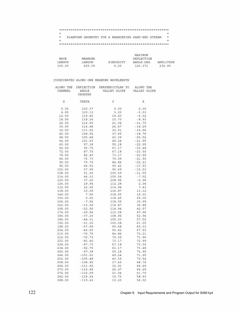
minimum stream power to uniquely define channel stability. An optional use of the analytical method is to assign a value for slope, thereby obtaining unique solutions for width and depth. Typically there will be two solutions for each slope. Meander Geometry Input The purpose of the meander calculations is to provide both curvilinear and Cartesian coordinates for a meander planform based on the sine-generated curve. The sine-generated curve has been shown to effectively replicate meander patterns in a wide variety of natural rivers. (Langbein and Leopold, 1966) Required input are the meander arc length and the meander wavelength, as shown in Figure 6.20. Title records are optional. The Meander arc length is the actual length of the channel, whereas the wavelength is the length, along the valley, of one full meander.

Figure 6.20. The Meander Calculation screen, with input. Output The output file first displays the SAM.hyd banner and echoes the input. An internal banner stresses that these calculations are appropriate for sand-be streams. The input wavelength and meander length are then printed along with the sinuosity, maximum deflection angle (in degrees), and the amplitude. Then a table of “Coordinates along one meander wavelength” is printed, giving the distance along the channel, deflection angle in degrees, the Y perpendicular to the valley slope, and the X along the valley slope.


********************************************************** * * * PLANFORM GEOMETRY FOR A MEANDERING SAND-BED STREAM * * * ********************************************************** MAXIMUM WAVE MEANDER DEFLECTION LENGTH LENGTH SINUOSITY ANGLE-DEG AMPLITUDE 100.00 600.00 6.00 120.371 236.90 COORDINATES ALONG ONE MEANDER WAVELENGTH ALONG THE DEFLECTION PERPENDICULAR TO ALONG THE CHANNEL ANGLE VALLEY SLOPE VALLEY SLOPE DEGREES S THETA Y X 0.00 120.37 0.00 0.00 6.00 120.13 5.20 -3.03 12.00 119.42 10.43 -6.02 18.00 118.24 15.70 -8.93 24.00 116.59 21.04 -11.70 30.00 114.48 26.47 -14.29 36.00 111.92 32.01 -16.66 42.00 108.92 37.65 -18.76 48.00 105.48 43.39 -20.54 54.00 101.63 49.24 -21.95 60.00 97.38 55.18 -22.95 66.00 92.75 61.17 -23.48 72.00 87.75 67.18 -23.50 78.00 82.40 73.17 -22.99 84.00 76.73 79.09 -21.90 90.00 70.75 84.86 -20.21 96.00 64.50 90.42 -17.93 102.00 57.99 95.69 -15.03 108.00 51.25 100.59 -11.55 114.00 44.31 105.04 -7.52 120.00 37.20 108.96 -2.96 126.00 29.94 112.28 2.04 132.00 22.56 114.94 7.43 138.00 15.09 116.87 13.12 144.00 7.56 118.05 19.01 150.00 0.00 118.45 25.00 156.00 -7.56 118.05 30.99 162.00 -15.09 116.87 36.88 168.00 -22.56 114.94 42.57 174.00 -29.94 112.28 47.96 180.00 -37.20 108.96 52.96 186.00 -44.31 105.03 57.52 192.00 -51.25 100.58 61.55 198.00 -57.99 95.68 65.03 204.00 -64.50 90.42 67.93 210.00 -70.75 84.86 70.21 216.00 -76.73 79.09 71.90 222.00 -82.40 73.17 72.99 228.00 -87.75 67.18 73.50 234.00 -92.75 61.17 73.48 240.00 -97.38 55.18 72.95 246.00 -101.63 49.24 71.95 252.00 -105.48 43.39 70.54 258.00 -108.92 37.65 68.76 264.00 -111.92 32.01 66.66 270.00 -114.48 26.47 64.29 276.00 -116.59 21.04 61.70 282.00 -118.24 15.70 58.93 288.00 -119.42 10.43 56.02


294.00 -120.13 5.20 53.03 300.00 -120.37 0.00 50.00 306.00 -120.13 -5.20 46.97 312.00 -119.42 -10.43 43.98 318.00 -118.24 -15.70 41.07 324.00 -116.59 -21.04 38.30 330.00 -114.48 -26.47 35.71 336.00 -111.92 -32.01 33.34 342.00 -108.92 -37.65 31.24 348.00 -105.48 -43.39 29.46 354.00 -101.63 -49.24 28.05 360.00 -97.38 -55.18 27.05 366.00 -92.75 -61.17 26.52 372.00 -87.75 -67.18 26.50 378.00 -82.40 -73.17 27.01 384.00 -76.73 -79.09 28.10 390.00 -70.75 -84.86 29.79 396.00 -64.50 -90.42 32.07 402.00 -57.99 -95.68 34.97 408.00 -51.25 -100.58 38.45 414.00 -44.31 -105.03 42.48 420.00 -37.20 -108.96 47.03 426.00 -29.94 -112.28 52.04 432.00 -22.56 -114.94 57.43 438.00 -15.09 -116.87 63.12 444.00 -7.56 -118.05 69.01 450.00 0.00 -118.45 75.00 456.00 7.56 -118.05 80.99 462.00 15.09 -116.87 86.88 468.00 22.55 -114.94 92.57 474.00 29.93 -112.28 97.96 480.00 37.20 -108.96 102.96 486.00 44.31 -105.04 107.52 492.00 51.25 -100.59 111.55 498.00 57.99 -95.69 115.03 504.00 64.50 -90.42 117.92 510.00 70.75 -84.86 120.21 516.00 76.73 -79.09 121.90 522.00 82.40 -73.17 122.99 528.00 87.75 -67.18 123.50 534.00 92.75 -61.17 123.48 540.00 97.38 -55.18 122.95 546.00 101.63 -49.24 121.95 552.00 105.48 -43.39 120.54 558.00 108.91 -37.65 118.76 564.00 111.92 -32.01 116.66 570.00 114.48 -26.47 114.29 576.00 116.59 -21.04 111.70 582.00 118.24 -15.70 108.93 588.00 119.42 -10.43 106.02 594.00 120.13 -5.20 103.03 600.00 120.37 0.00 100.00 This calculation has no plotting capability, but the table of coordinates could be copied into a spreadsheet for plotting.

Date post:	28-Dec-2019
Category:	Documents
Upload:	others
View:	22 times
Download:	0 times

6 Input Requirements and Program Output for SAMChapter 6 Input Requirements and Program Output for...

Documents