6 Insurances on Joint Lives 6.1 Introduction It is common for life insurance policies and annuities to depend on the death or survival of more than one life. For example: (i) A policy which pays a monthly benefit to a wife or other dependents after the death of the husband (widow’s or dependent’s pension). (ii) A policy which pays a lump-sum on the second death of a couple (often to meet inheritance tax liability). We will confine attention to policies involving two livesbut the same approaches can be extended to any number of lives. We assume that policies are sold to a life age x and a life age y , denoted (x) and (y ). The basic contract types we will consider are: • Assurances paying out on first death, and annuities payable until first death. 131
Transcript
6 Insurances on Joint Lives
6.1 Introduction
It is common for life insurance policies and annuities to depend on the death or survival of
more than one life. For example:
(i) A policy which pays a monthly benefit to a wife or other dependents after the death of
the husband (widow’s or dependent’s pension).
(ii) A policy which pays a lump-sum on the second death of a couple (often to meet
inheritance tax liability).
We will confine attention to policies involving two livesbut the same approaches can be
extended to any number of lives. We assume that policies are sold to a life age x and a life
age y, denoted (x) and (y).
The basic contract types we will consider are:
• Assurances paying out on first death, and annuities payable until first death.
131
• Assurances paying out on second death, and annuities payable until second death.
• Assurances and annuities whose payment depends on the order of deaths.
6.2 Multiple-state model for two lives
The following multiple-state model represents the joint mortality of two lives, (x) and (y).
State 3(x) Alive(y) Dead
State 4(x) Dead(y) Dead
-
State 1(x) Alive(y) Alive
State 2(x) Dead(y) Alive
µ34
t
µ12
t-
µ13
t
?
µ24
t
?
132
Notes:
• We just index the transition intensities by time t. Other notations are possible.
• We implicitly assume that the simultaneous death of (x) and (y) is impossible: there
is no direct transition from state 1 to state 4.
Here we list the main EPVs met in practice, giving their symbols in the standard actuarial
notation. In the first place, we assume all insurance contracts (assurance- or annuity-type)
to be for all of lifeand to be of unit amount, i.e. $1 sum assured or $1 annuity per
annum.
Joint-life assurances
• Axy is the EPV of $1 paid immediately on the first death of (x) or (y).
• Axy is the EPV of $1 paid immediately on the second death of (x) and (y).
133
Contingent assurances
• A1xy is the EPV of $1 paid immediately on the death of (x)provided (y) is then alive,
i.e. provided (x) is the first to die.
• A 1xy is the EPV of $1 paid immediately on the death of (y)provided (x) is then alive,
i.e. provided (y) is the first to die.
• A2xy is the EPV of $1 paid immediately on the death of (x)provided (y) is then dead,
i.e. provided (x) is the second to die.
• A 2xy is the EPV of $1 paid immediately on the death of (y)provided (x) is then dead,
i.e. provided (y) is the second to die.
Joint-life annuities
• axy is the EPV of an annuity of $1 per annum, payable continuously, until the first of
(x) or (y) dies.
134
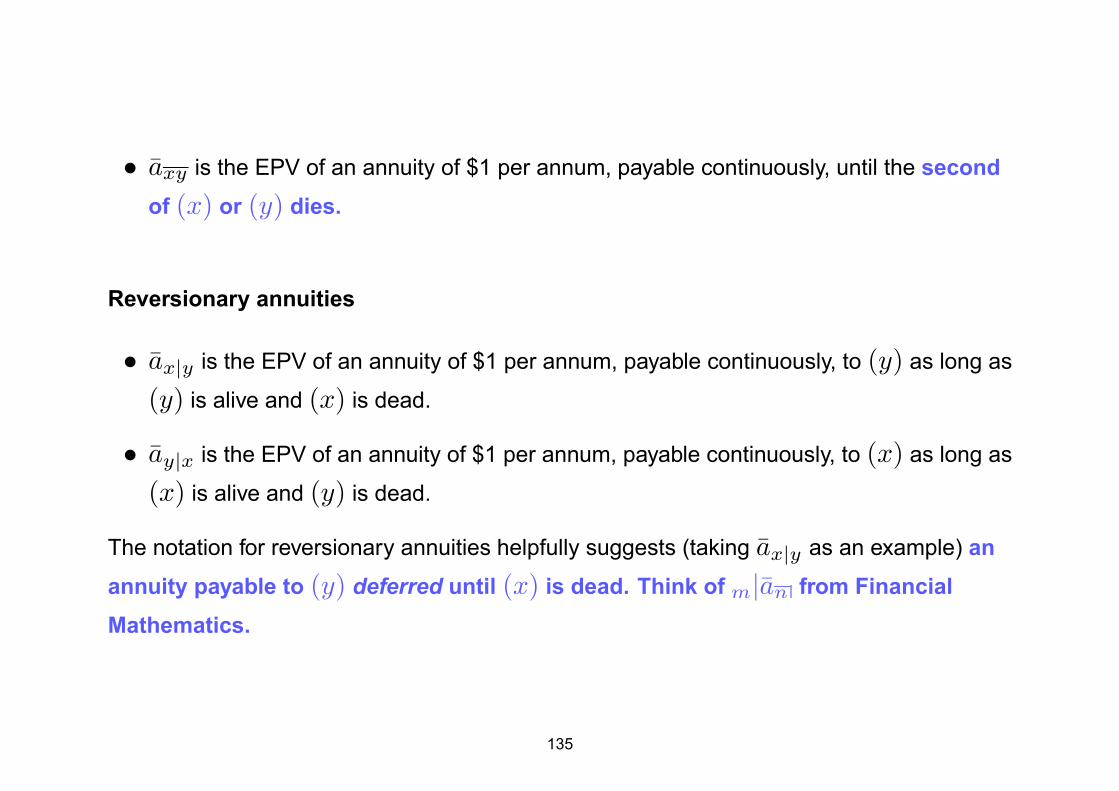
• axy is the EPV of an annuity of $1 per annum, payable continuously, until the second
of (x) or (y) dies.
Reversionary annuities
• ax|y is the EPV of an annuity of $1 per annum, payable continuously, to (y) as long as
(y) is alive and (x) is dead.
• ay|x is the EPV of an annuity of $1 per annum, payable continuously, to (x) as long as
(x) is alive and (y) is dead.
The notation for reversionary annuities helpfully suggests (taking ax|y as an example) an
annuity payable to (y) deferred until (x) is dead. Think of m|an from Financial
Mathematics.
135
Limited terms
The above contracts may all be written for a limited term of n years, in which case the
usual n is appended to the subscript.
Evaluation of EPVs
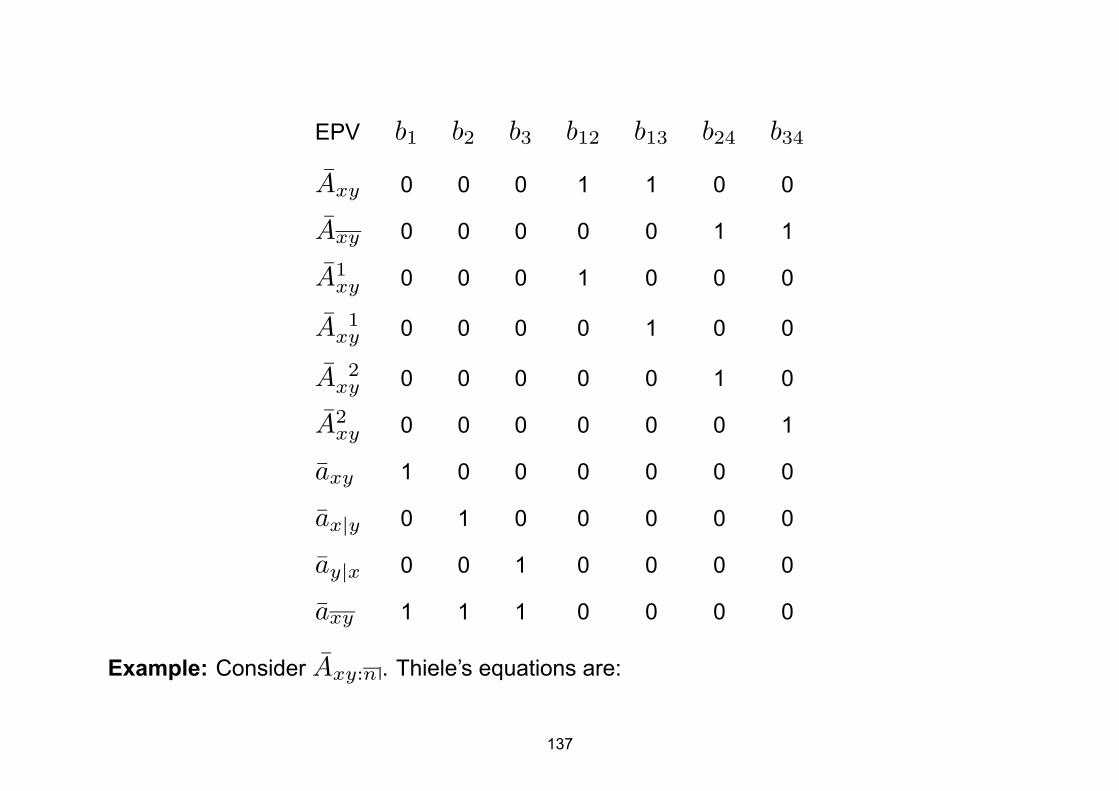
In the multiple-state, continuous-time model, we can compute all the above EPVs simply by
appropriate choices of assurance benefits bij or annuity benefits biin Thiele’s
differential equations. The following table lists these choices for whole-life contracts.
136
EPV b1 b2 b3 b12 b13 b24 b34
Axy 0 0 0 1 1 0 0
Axy 0 0 0 0 0 1 1
A1xy 0 0 0 1 0 0 0
A 1xy 0 0 0 0 1 0 0
A 2xy 0 0 0 0 0 1 0
A2xy 0 0 0 0 0 0 1
axy 1 0 0 0 0 0 0
ax|y 0 1 0 0 0 0 0
ay|x 0 0 1 0 0 0 0
axy 1 1 1 0 0 0 0
Example: Consider Axy:n . Thiele’s equations are:
137
d
dtV 1(t) = V 1(t) δ − (µ12
t + µ13t )(1− V 1(t))
d
dtV 2(t) =
d
dtV 3(t) =
d
dtV 4(t) = 0
with boundary conditions V 1(n) = 1 and all other V i(n) = 0.
Composite benefits
Many joint life contracts can be built up out of the above EPVs and the EPVs of single life
benefits. This is generally the simplest way to compute them, especially if using tables
rather than a spreadsheet.
Example: Consider a pension of $10,000 per annum, payable continuously as long as (x)
and (y) are alive, reducing by half on the death of (x) if (x) dies before (y). (This would
be a typical retirement pension with a spouse’s benefit.)Its EPV, denoted a say, is most
easily computed by noting that $10,000 p.a. is payable as long as (x) is alive, and in
138
addition, $5,000 p.a. is payable if (y) is alive but (x) is dead, hence:
a = 10, 000 ax + 5, 000 ax|y.
By similar reasoning, an annuity of $1 p.a. payable to (y) for life can be decomposed into
an annuity of $1 p.a. payable until the first death of (x) and (y), plus a reversionary
annuity of $1 p.a. payable to (y) after the prior death of (x); hence the useful:
ax|y = ay − axy.
Computing contingent assurance EPVs
The one type of joint life benefit whose EPV is not easily written in terms of first-death,
second-death and single-life EPVs is the contingent assurance. We defer discussion until
139
Section 6.4.
6.3 Random joint lifetimes
It is also possible to specify a joint lives model via random future lifetimes. We have the
random variables:
Tx = the future lifetime of (x)
Ty = the future lifetime of (y).
Now define the random variables:
Tmin = min(Tx, Ty) and
Tmax = max(Tx, Ty).
Tmin is the random time until the first death occurs, and Tmax is the random time until the
140
second death occurs.
The distribution of Tmin
Define:
tqxy = P {Tmin ≤ t} (c.d.f.)
tpxy = P {Tmin > t}
So that: tqxy + tpxy = 1.
Now if Tx and Ty are independent:
tpxy = P {Tmin > t}
= P {Tx > t and Ty > t}
= P {Tx > t} × P {Ty > t}
= tpx tpy
141
and (useful result) the joint life survival function tpxy is the product of the single life
survival functions.
If Tx and Ty are not independent then we cannot write tpxy = tpx tpy .
If Tx and Ty are independent then also:
tqxy = 1− tpxy
= 1− tpx tpy
= 1− {(1− tqx)(1− tqy)}
= tqx + tqy − tqx tqy.
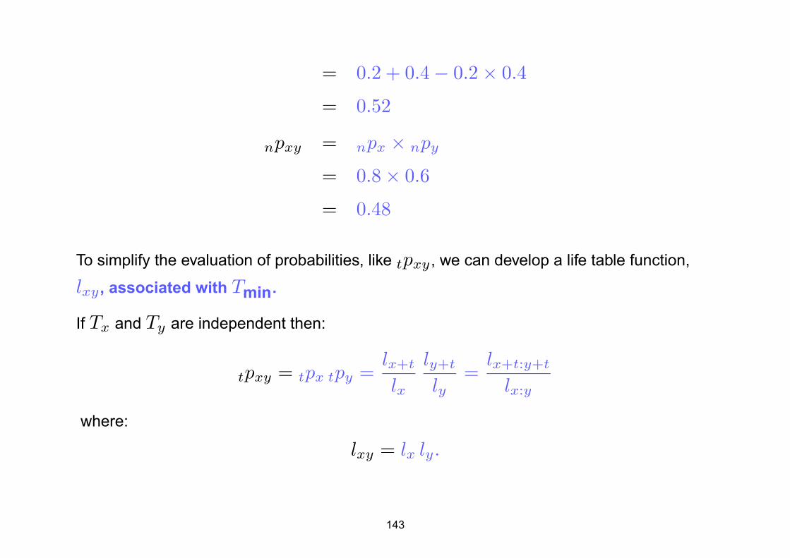
Example: Given nqx = 0.2 and nqy = 0.4
calculate nqxy and npxy .
Solution:
nqxy = nqx + nqy − nqx nqy
142
= 0.2 + 0.4− 0.2× 0.4
= 0.52
npxy = npx × npy
= 0.8× 0.6
= 0.48
To simplify the evaluation of probabilities, like tpxy , we can develop a life table function,
lxy , associated with Tmin.
If Tx and Ty are independent then:
tpxy = tpx tpy =lx+t
lx
ly+t
ly=
lx+t:y+t
lx:y
where:
lxy = lx ly.
143
We obtain the p.d.f. of Tmin, denoted fxy(t), by differentiation when Tx and Ty are
independent:
fxy(t) =d
dttqxy
= −d
dttpxy
= −d
dttpx · tpy
= −
[
tpx
d
dttpy + tpy
d
dttpx
]
= − [tpx (−tpyµy+t) + tpy (−tpxµx+t)]
= tpxy (µx+t + µy+t).
144
Compare this to the single life case:
fx(t) = tpx µx+t.
Now, define µxy(t) as the ‘force of mortality’ associated with Tmin. We can show directly
that
µxy(t) = µx+t + µy+t
when Tx and Ty are independent because:
µxy(t) =fxy(t)
tpxy
= µx+t + µy+t.
However, using the multiple-state formulation of the model, we see that Tmin is just the
145
time when state 1 is left.The survival function associated with this event is, by definition,
tp11• (where the bullet represents policy inception) and we know that:
tp11• = exp
(
−
∫ t
0
µ12s + µ13
s ds
)
.
By differentiating this, the ‘force of mortality’ associated with leaving state 1 is the sum of
the intensities out of state 1 without assuming that Tx and Ty are independent.
The distribution of Tmax
Define:
tqxy = P {Tmax ≤ t} (c.d.f.)
tpxy = P {Tmax > t}
So that tqxy + tpxy = 1. We have:
146
tpxy = P{Tmax > t)}
= P{Tx > t or Ty > t}
= P{Tx > t}+ P{Ty > t}
− P{Tx > t and Ty > t}
= tpx + tpy − tpxy
which does not require Tx and Ty to be independent. If they are independent then:
tpxy = tpx + tpy − tpx tpy
and also:
tqxy = P{Tmax ≤ t}
147
= P {Tx ≤ t and Ty ≤ t}
= P{Tx ≤ t}P{Ty ≤ t} = tqx tqy.
The p.d.f. of Tmax and the ‘force of mortality’ µxy(t)associated with Tmax are left as
tutorial questions.
Expectations of joint lifetimes
Define:◦exy = E[Tmin] and
◦exy = E[Tmax].
Now, consider the following identities:
Identity 1 Tmin + Tmax = Tx + Ty .
Identity 2 TminTmax = TxTy .
148
These can be verified by considering the three exhaustive and exclusive cases:
Tx > Ty, Tx < Ty and Tx = Ty.
Taking expectations of the first identity gives:
E [Tmin + Tmax] = E [Tx + Ty]
=⇒ E [Tmin] + E [Tmax] = E [Tx] + E [Ty]
=⇒◦exy +
◦exy =
◦ex +
◦ey.
¿From the second identity we have:
E [Tmin Tmax] = E [Tx Ty]
and if Tx and Ty are independent we have:
E [Tmin Tmax] = E [Tx] E [Ty] .
149
Evaluation of EPVs
We can evaluate EPVs using the distributions of Tmin and Tmax, just as for a single life,
as an alternative to solving Thiele’s equations. For example, consider an assurance with a
sum assured of $1 payable immediately on the first death of (x) and (y).
The PV of benefits = vTmin
with p.d.f. = tpxy µxy(t)
so the expected present value Axy is:
Axy = E
[
vTmin]
=
∫ ∞
0
vttpxy µxy(t) dt.
Note that evaluating an integral numerically is not significantly easier than solving Thiele’s
equations numerically.
150
6.4 Curtate Future Joint Lifetimes
Basic definitions
We now introduce discrete random variables. Let:
Kmin = Integer part of Tmin
Kmax = Integer part of Tmax.
We can then define the curtate expectation of life as:
exy = E [Kmin]
exy = E [Kmax] .
For more properties of exy and exy see tutorial.
The associated deferred probabilities k
∣∣qxy and k
∣∣qxy (i.e. the distribution functions of
151
Kmin and Kmaxare given by:
k
∣∣qxy = P {k ≤ Tmin < k + 1}
= P {Kmin = k}
k
∣∣qxy = P {k ≤ Tmax < k + 1}
= P {Kmax = k} .
Example: Given:
tqnon-smokerx =
70− x + t
80− x
valid for 0 ≤ x ≤ 70 and 0 ≤ t ≤ 10, and that the force of mortality for smokers is twice
that for non-smokers, calculate the expected time to first death of a (70) smoker and a (70)
non-smoker. You are given that the lives are independent.
152
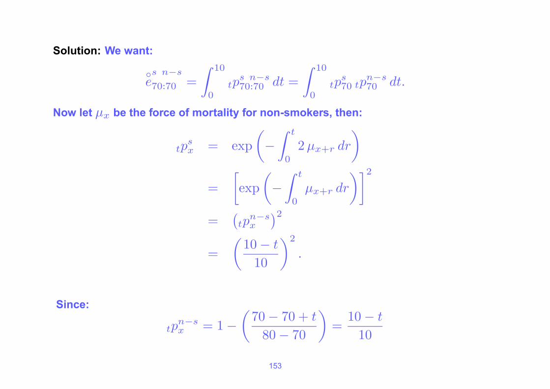
Solution: We want:
◦es n−s
70:70 =
∫ 10
0tp
s n−s70:70 dt =
∫ 10
0tp
s70 tp
n−s70 dt.
Now let µx be the force of mortality for non-smokers, then:
tpsx = exp
(
−
∫ t
0
2 µx+r dr
)
=
[
exp
(
−
∫ t
0
µx+r dr
)]2
=(
tpn−sx
)2
=
(10− t
10
)2
.
Since:
tpn−sx = 1−
(70− 70 + t
80− 70
)
=10− t
10
153
therefore:
◦es n−s
70:70 =
∫ 10
0
[10− t
10
]3
dt = 2.5 years.
Discrete joint life annuities
Any annuity or assurance we can define as a function of the single lifetime Kx, we can
define using Kmin, therefore depending on the first deathor Kmax, therefore
depending on the second death.
Example: Consider an annuity of $1 per annum, payable yearly in advance in advanceas
long as both (x) and (y) are alive (i.e. payable until the first death).The same reasoning
as in the single-life case shows that the present value of this is:
PV = aKmin+1 .
154
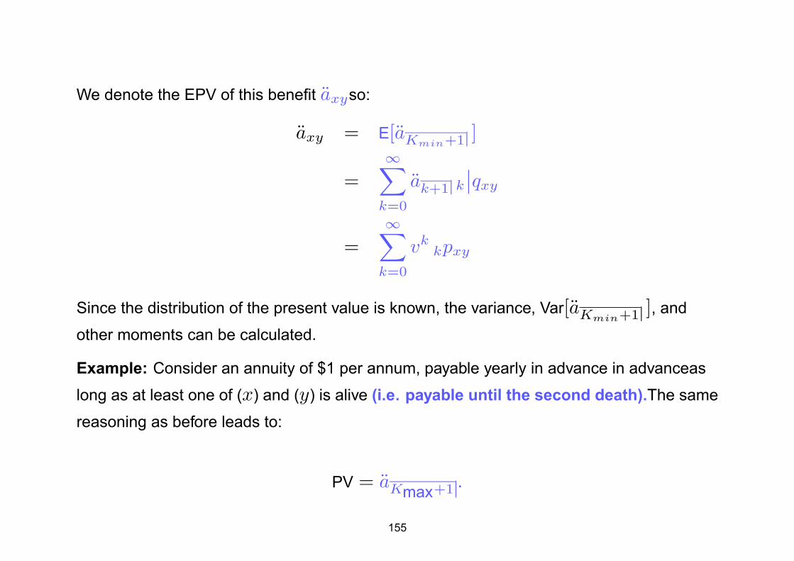
We denote the EPV of this benefit axyso:
axy = E[aKmin+1 ]
=∞∑
k=0
ak+1 k
∣∣qxy
=∞∑
k=0
vkkpxy
Since the distribution of the present value is known, the variance, Var[aKmin+1 ], and
other moments can be calculated.
Example: Consider an annuity of $1 per annum, payable yearly in advance in advanceas
long as at least one of (x) and (y) is alive (i.e. payable until the second death).The same
reasoning as before leads to:
PV = aKmax+1 .
155
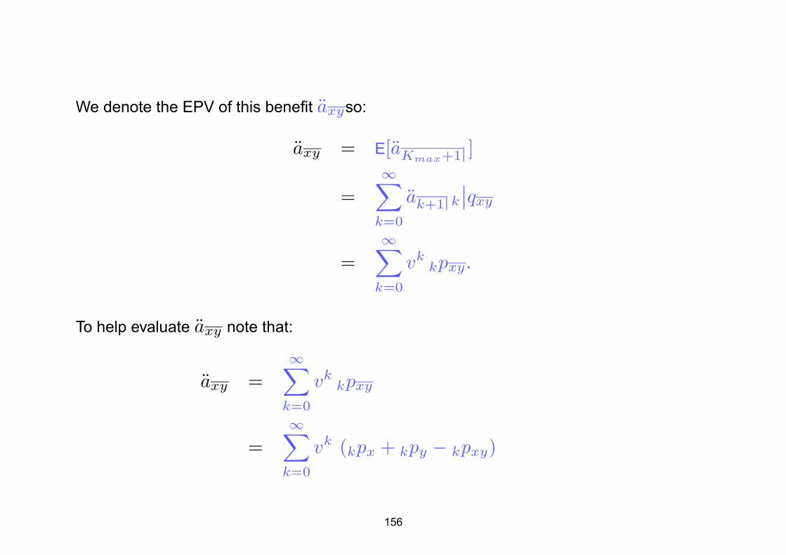
We denote the EPV of this benefit axyso:
axy = E[aKmax+1 ]
=∞∑
k=0
ak+1 k
∣∣qxy
=∞∑
k=0
vkkpxy.
To help evaluate axy note that:
axy =∞∑
k=0
vkkpxy
=∞∑
k=0
vk (kpx + kpy − kpxy)
156
=∞∑
k=0
vkkpx +
∞∑
k=0
vkkpy −
∞∑
k=0
vkkpxy
= ax + ay − axy.
Hence also:
axy + axy = ax + ay.
Computing axy etc. using tables
It is easy to compute EPVs of discrete benefits using a spreadsheet if tpxy is known,
which is particularly simple if Tx and Ty are independent so tpxy = tpx tpy .
However, other methods can be used if joint life tablesare available, as they will be in
examinations.
(i) Given tabulated values of axy directly.
157
e.g. a(55) tables, but note that the values of axy are given not axy , and they are only
given for even ages — may need to use linear interpolation.
For example:
a66:61 ≈1
2(a66:60 + a66:62).
(ii) Given commutation functions. e.g. A1967–70 tables, but note that they are only given
for x = y and at 4% interest.
Note that (assuming independence):
axy =∞∑
t=0
vttpxy =
∞∑
t=0
vttpx tpy
=∞∑
t=0
{
vt lx+t ly+t
lx ly
}
158
=∞∑
t=0
{
v1
2(x+y)+t lx+t ly+t
v1
2(x+y) lx ly
}
=Nxy
Dxy
where:
Dxy = v1
2(x+y) lx ly
Nx+t:y+t =∞∑
r=0
Dx+t+r: y+t+r.
159
Warning:
axy:n = axy − n
∣∣axy
= axy − vnnpx npy ax+n:y+n
= axy −1
vn
Dx+n Dy+n
Dx Dy
ax+n:y+n.
Example: Using a(55) mortality and 6% interest calculate the following:
(i) a80:75
(ii) 10| a70:65.
Solution:
a80:75 = 0.5(a80:74 + a80:76)
= 0.5(1 + a80:74 + 1 + a80:76)
= 0.5(4.395 + 4.538) = 4.467.
160
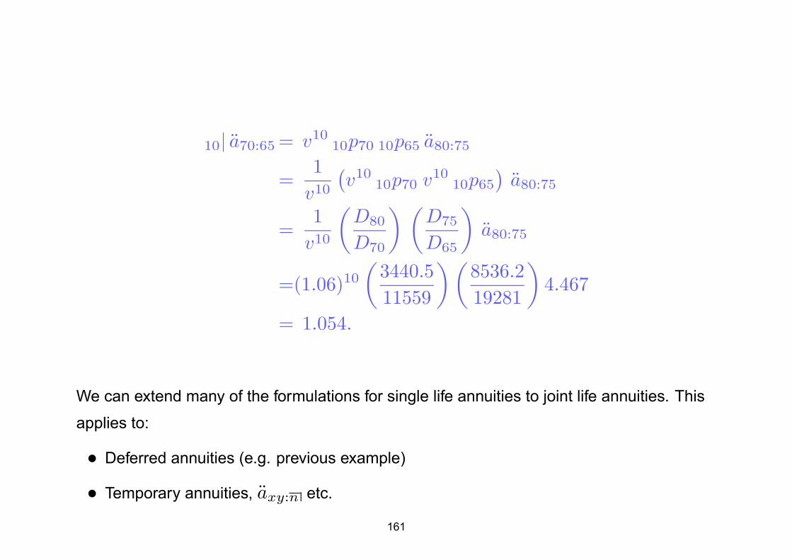
10| a70:65 = v1010p70 10p65 a80:75
=1
v10
(v10
10p70 v1010p65
)a80:75
=1
v10
(D80
D70
) (D75
D65
)
a80:75
=(1.06)10(
3440.5
11559
)(8536.2
19281
)
4.467
= 1.054.
We can extend many of the formulations for single life annuities to joint life annuities. This
applies to:
• Deferred annuities (e.g. previous example)
• Temporary annuities, axy:n etc.
161
• Increasing annuities, (Ia)xy etc.
• Annuities paid monthly. For example:
a(m)xy ≈ axy −
m− 1
2m.
• Approximations for annuities paid continuously. For example:
axy ≈ axy − 0.5 = axy + 0.5.
Example (Question No 8 Diploma Paper June 1997):
A certain life office issues a last survivor annuity of $2,000 per annum, payable annually in
arrear, to a man aged 68 and a woman aged 65.
(a) Using the a(55) ultimate table (male/female as appropriate) and a rate of interest of
4% per annum, estimate the expected present value of this benefit.
(b) Using the basis of (a) above, derive an expression (which you need NOT evaluate)
162
for the standard deviation of the present value of this benefit, in terms of single life
and joint life annuity functions.
Solution:
(a) We want: 2000 am f
68:65
= 2000(
am68 + a
f65 − a
m f68:65
)
≈ 2000
(
am68 + a
f65 −
1
2
(
am f68:64 + a
m f68:66
))
= 2000 (8.688 + 11.497
−1
2(7.418 + 7.186)
)
= 25, 766.00.
163
(b) Present Value = 2000 aKmax
So we want: Var
[
2000 aKmax
]
= 20002Var
[
aKmax+1 − 1]
= 20002Var
[
aKmax+1
]
= 20002Var
[1− vKmax+1
d
]
=
(2000
d
)2
Var[vKmax+1
]
=
(2000
d
)2 (
∗Am f
68:65−
(
Am f
68:65
)2)
164
where * means evaluated at:
j = i2 + 2i = 8.16%.
We now use:
Axy = 1− d axy
and:
axy = ax + ay − axy
and:
SD[PV ] =√
V ar[PV ]
to get:
2000
d
{
1− ∗d(∗am
68 + ∗af65 −
∗am f68:65
)
−[
1− d(
am68 + a
f65 − a
m f68:65
)]2} 1
2
.
165
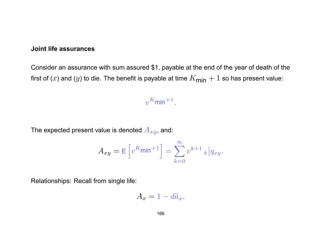
Joint life assurances
Consider an assurance with sum assured $1, payable at the end of the year of death of the
first of (x) and (y) to die. The benefit is payable at time Kmin + 1 so has present value:
vKmin+1.
The expected present value is denoted Axy , and:
Axy = E
[
vKmin+1]
=
∞∑
k=0
vk+1k
∣∣qxy.
Relationships: Recall from single life:
Ax = 1− dax.
166
It can be shown by similar reasoning that:
Axy = 1− daxy
Axy = 1− δ axy
Axy:n = 1− daxy:n
Axy:n = 1− δ axy:n
and so on.
Associated with the second death we have:
Axy = E[vKmax+1] =∞∑
k=0
vk+1k| qxy
167
and similar relationships can be derived, e.g:
Axy = 1− daxy
Axy:n = 1− daxy:n .
Reversionary Annuities
We noted before that:
ax|y = ay − axy
just by noticing that the following define identical cashflows no matter when (x) and (y)
should die:
(1) a reversionary annuity of $1 per annum payable continuously while (y) is alive,
following the death of (x).
(2) an annuity of $1 per annum payable continuously to (y) for life, less an annuity of $1
168
per annum payable continuously until the first death of (x) and (y).
Hence the cashflows have identical present values, and the same EPVs. We can apply
similar reasoning to other variants of reversionary annuities, for example:
ax|y = ay − axy
=∞∑
k=0
vkkpy(1− kpx)
ax|y = ay − axy
=∞∑
k=1
vkkpy(1− kpx)
a(m)x|y = a(m)
y − a(m)xy
=1
m
∞∑
k=0
vk
m k
m
py(1− k
m
px)
169
a(m)x|y = a(m)
y − a(m)xy
=1
m
∞∑
k=1
vk
m k
m
py(1− k
m
px).
We can take advantage of some relationships to simplify calculations.
For example:
ax|y = ay − axy
= (1 + ay)− (1 + axy)
= ay − axy.
Hence:
ax|y = ax|y.
Similarly, we can derive other relationships like:
170
(a) ax|y ≈ ax|y
(b) a(m)x|y ≈ ax|y.
Example: Calculate the annual premium (payable while both lives are alive) for the
following contract for a man aged 70 and woman aged 64.
Benefits:
• SA of $10,000 payable immediately on first death; and
• a reversionary annuity of $5,000 payable
continuously to the survivor for the remainder of their lifetime.
Basis:
• Renewal expenses 10% of all premiums.
• a(55) Ultimate, male/female as appropriate
• Interest at 8%.
171
Solution: Let P = Annual Premium.
EPV of premiums less expenses
= 0.9 P am f70:64
= 0.9 P (1 + 5.576)
= 5.9184 P.
EPV of assurance
= 10, 000Am f70:64
= 10, 000(
1− δ am f70:64
)
≈ 10, 000(
1− 0.076961(am f70:64 + 0.5)
)
= 10, 000 (1− 0.076961(5.576 + 0.5))
= 5, 323.85.
172
EPV of reversionary annuity
= 5, 000(
am f
70|64 + af m
64|70
)
= 5, 000(
am f
70|64 + af m
64|70
)
= 5, 000(
af64 − a
m f70:64 + am
70 − af m64:70
)
= 5, 000 (8.574 + 6.268− 2× 5.576)
= 18, 450.0.
Now set: EPV[Income] = EPV[Outgo]
=⇒ 5.9184 P = 5, 323.85 + 18, 450.0
=⇒ P = 4, 016.94.
173
Contingent assurances
Consider a contingent assurance with sum assured $1 payable immediately on the death
of (x), if (y) is still then alive.
The probability that life (x) dies within t years with life (y) being alive when life (x) dies is
denoted tq1xyand:
tq1xy = P[(x) dies within t years and before (y)]
= P[Tx < t and Tx < Ty].
This is an example of a contingent probability,so called because they are associated with
the death of a life contingent on the survival or death of another life.
Now let fx(r) be the density of Tx and fy(r) be the density of Ty , then:
tq1xy =
∫ t
r=0
∫ ∞
s=r
fx(r)fy(s)ds dr
174
=
∫ t
r=0
fx(r)
[∫ ∞
s=r
fy(s)ds
]
dr.
Since: ∫ ∞
s=r
fy(s)ds = rpy
then:
tq1xy =
∫ t
r=0rpx µx+r rpy dr.
Illustration: (x) survives to time r and then dies and (y) survives beyond r, giving:
rpx µx+r rpy
-| |Age
︷ ︸︸ ︷
(x) survives = rpx
?
(x) dies = µx+r
| -(y) survives = rpy
x
y
x + r
y + r175
Note that since one of (x) and (y) has to die first:
tq1xy + tq
1xy = tqxy.
We define tq2xy as the probability that (x) dies within t years but after (y) has died.
Therefore:
tqx = tq1xy + tq
2xy
from which:
tq2xy =
∫ t
0rpx µx+r (1− rpy) dr.
With these probabilities we can now evaluate the EPV A1xy .
A1xy =
vTx if Tx < Ty
0 if Tx ≥ Ty.
176
¿From this it can be shown that:
A1xy =
∫ ∞
0
vrrpx µx+r rpy dr.
Similarly, we can derive an expression for the EPV of a benefit of $1 payable immediately
on the death of (x) if it is after that of (y), denoted A2xy :
A2xy =
∫ ∞
0
vrrpx µx+r (1− rpy) dr.
We see, what is intuitively clear, that:
Ax = A1xy + A2
xy.
Other important relationships:
(a) Axy = A1xy + A 1
xy and Axy = A2xy + A 2
xy .
177
(b) A1xy =
∞∑
t=0
vt+1tpxtpy · q
1x+t:y+t.
(c) Axy = A1xy + A 1
xy and Axy = A2xy + A 2
xy .
(d) A1xy ≈ (1 + i)−
1
2 A1xy .
If the two lives are the same age, and the same mortality table is applies to both, then:
A1xx =
1
2Axx
A1xx =
1
2Axx
A2xx =
1
2Axx
A2xx =
1
2Axx.
178
6.5 Examples
Example 1
Find the expected present value of an annuity of $10,000 p.a. payable annually in advance
to a man aged 65, reducing to $5,000 p.a. continuing in payment to his wife, now aged 61,
if she survives him.
Basis:
• Mortality — a(55) ultimate, male/female as appropriate
• Interest: 8% p.a.
• Ignore the possibility of divorce.
Solution
EPV
= 10, 000 am65 + 5, 000 a
m f
65|61
= 10, 000 (am65 + 1) + 5, 000 a
m f
65|61
179
= 10, 000 (7.4 + 1) + 5, 000(
af61 − a
m f65:61
)
= 10, 000 (8.4) + 5, 000 (9.124− 6.619)
= 96, 525.
Since:
am f65:61 ≈
1
4
(
am f66:62 + a
m f66:60 + a
m f64:62 + a
m f64:60
)
=1
4(6.392 + 6.519 + 6.709 + 6.854)
= 6.619.
Example 2
(a) Express nq 2xy in terms of single life probabilities and contingent probabilities
referring to the first death.
(b) Suppose µx = 180−x
for 0 ≤ x ≤ 80,
180
evaluate 20q2
40:50.
Solution
(a) tq2
xy
=
∫ t
r=0rpy µy+r (1− rpx) dr
=
∫ t
r=0rpy µy+r dr −
∫ t
r=0rpy µy+r rpx dr
= tqy − tq1
xy.
(b) nqx = 1− npx
= 1− exp
{
−
∫ n
0
µx+t dt
}
181
= 1− exp
{
−
∫ n
0
1
80− x− tdt
}
= 1− exp {[log (80− x− t)]n
0}
= 1− exp
{
log
(80− x− n
80− x
)}
=n
80− x.
and we have nq 1xy
=
∫ n
0tpx tpy µy+t dt
=1
(80− x)(80− y)
∫ n
0
(80− x− t) dt
=n (80− x)− 1
2n2
(80− x)(80− y)
182
∴ 20q2
40:50 = 20q50 − 20q1
40:50
=20
30−
20× 40− 12 202
40× 30
=1
6.
Example 3
Consider a reversionary annuity of $1 p.a. payable quarterly in advance during the lifetime
of (y) following the death of (x). Show that the expected present value of this benefit is
approximately equal to:
ax|y +1
8A1
xy.
Solution
Hint: Fix a time t to represent the death of (x), as below: