6 Least Squares, Fourier Analysis, and Related Approximation Norms • • • Up to this point we have required that any function we use to represent our 'data' points pass through those points exactly. Indeed, except for the predictor-corrector schemes for differential equations, we have used all the information available to determine the approximating function. In the extreme case of the Runge-Kutta method, we even made demands that exceeded the available information. This led to approximation formulae that were under-determined. Now we will consider approaches for determining the approximating function where some of the information is deliberately ignored. One might wonder why such a course would ever be followed. The answer can be found by looking in two rather different directions. 159
Transcript
6 Least Squares, Fourier
Analysis, and Related Approximation Norms
• • • Up to this point we have required that any function we use to represent our 'data' points pass through those points exactly. Indeed, except for the predictor-corrector schemes for differential equations, we have used all the information available to determine the approximating function. In the extreme case of the Runge-Kutta method, we even made demands that exceeded the available information. This led to approximation formulae that were under-determined. Now we will consider approaches for determining the approximating function where some of the information is deliberately ignored. One might wonder why such a course would ever be followed. The answer can be found by looking in two rather different directions.
159
Numerical Methods and Data Analysis
Remember, that in considering predictor-corrector schemes in the last chapter, we deliberately ignored some of the functional values when determining the parameters that specified the function. That was done to avoid the rapid fluctuations characteristic of high degree polynomials. In short, we felt that we knew something about extrapolating our approximating function that transcended the known values of specific points. One can imagine a number of situations where that might be true. Therefore we ask if there is a general approach whereby some of the functional values can be deliberately ignored when determining the parameters that represent the approximating function. Clearly, anytime the form of the function is known this can be done. This leads directly to the second direction where such an approach will be useful. So far we have treated the functional values that constrain the approximating function as if they were known with absolute precision. What should we do if this is not the case? Consider the situation where the functional values resulted from observation or experimentation and are characterized by a certain amount of error. There would be no reason to demand exact agreement of the functional form at each of the data points. Indeed, in such cases the functional form is generally considered to be known a priori and we wish to test some hypothesis by seeing to what extent the imprecise data are represented by the theory. Thus the two different cases for this approach to approximation can be summarized as: a. the data is exact but we desire to represent it by an approximating function with fewer
parameters than the data. b. the approximating function can be considered to be "exact" and the data which represents
that function is imprecise. There is a third situation that occasionally arises wherein one wishes to approximate a table of empirically determined numbers which are inherently imprecise and the form of the function must also be assumed. The use of any method in this instance must be considered suspect as there is no way to separate the errors of observation or experimentation from the failure of the assumed function to represent the data. However, all three cases have one thing in common. They will generate systems that will be over-determined since there will, in general, be more constraining data than there are free parameters in the approximating function. We must then develop some criterion that will enable us to reduce the problem to one that is exactly determined. Since the function is not required to match the data at every point, we must specify by how much it should miss. That criterion is what is known as an approximation norm and we shall consider two popular ones, but devote most of our effort to the one known as the Least Square Norm. 6.1 Legendre's Principle of Least Squares Legendre suggested that an appropriate criterion for fitting data points with a function having fewer parameters than the data would be to minimize the square of the amount by which the function misses the data points. However, the notion of a "miss" must be quantified. For least squares, the "miss" will be considered to result from an error in the dependent variable alone. Thus, we assume that there is no error in the independent variable. In the event that each point is as important as any other point, we can do this by minimizing the sum-square of those errors. The use of the square of the error is important for it eliminates the influence of its sign. This is the lowest power dependence of the error ε between the data point and the
160
6 - Least Squares
approximating function that neglects the sign. Of course one could appeal to the absolute value function of the error, but that function is not continuous and so may produce difficulties as one tries to develop an algorithm for determining the adjustable free parameters of the approximating function. Least Squares is a very broad principle and has special examples in many areas of mathematics. For example, we shall see that if the approximating functions are sines and cosines that the Principle of Least Squares leads to the determination of the coefficients of a Fourier series. Thus Fourier analysis is a special case of Least Squares. The relationship between Least Squares and Fourier analysis suggests a broad approximation algorithm involving orthogonal polynomials known as the Legendre Approximation that is extremely stable and applicable to very large data bases. With this in mind, we shall consider the development of the Principle of Least Squares from several different vantage points. There are those who feel that there is something profound about mathematics that makes this the "correct" criterion for approximation. Others feel that there is something about nature that makes this the appropriate criterion for analyzing data. In the next two chapters we shall see that there are conditions where the Principle of Least Squares does provide the most probable estimate of adjustable parameters of a function. However, in general, least squares is just one of many possible approximation norms. As we shall see, it is a particularly convenient one that leads to a straightforward determination of the adjustable free parameters of the approximating function. a. The Normal Equations of Least Squares Let us begin by considering a collection of N data points (xi,Yi) which are to be represented by an approximating function f(aj,x) so that
f(aj, xi ) = Yi . (6.1.1) Here the (n+1) aj's are the parameters to be determined so that the sum-square of the deviations from Yi are a minimum. We can write the deviation as
εi = Yi ─ f(aj,xi) . (6.1.2) The conditions that the sum-square error be a minimum are just
∑∑
=
==∂
∂−=
∂
ε∂ N
1i j
ijiji
i
N
i
2i
n,,2,1,0j,0a
)x,a(f)]x,a(fY[2
aL . (6.1.3)
There is one of these equations for each of the adjustable parameters aj so that the resultant system is uniquely determined as long as (n+1) N. These equations are known as the normal equations for the problem. The nature of the normal equations will be determined by the nature of f(aj,x). That is, should f(aj,x) be non-linear in the adjustable parameters aj, then the normal equations will be non-linear. However, if f(aj,x) is linear in the aj's as is the case with polynomials, then the resultant equations will be linear in the aj's. The ease of solution of such equations and the great body of literature relating to them make this a most important aspect of least squares and one on which we shall spend some time.
161
Numerical Methods and Data Analysis
b. Linear Least Squares Consider the approximating function to have the form of a general polynomial as described in chapter 3 [equation (3.1.1)]. Namely
∑=
φ=n
0kkkj )x(a)x,a(f φ . (6.1.4)
Here the φk(x) are the basis functions which for common polynomials are just xk. This function, while highly non-linear in the independent variable x is linear in the adjustable free parameters ak. Thus the partial derivative in equation (6.1.3) is just
)x(a
)x,a(fij
j
ij φ=∂
∂ , (6.1.5)
and the normal equations themselves become
∑ ∑ ∑= = =
=φ=φφn
0k
N
1i
N
1iijiijikk n,,1,0j,)x(Y)x()x(a L . (6.1.6)
These are a set of linear algebraic equations, which we can write in component or vector form as
⎪⎭
⎪⎬⎫
=•
=∑Ca
CAak
jkjk
rr A . (6.1.7)
Since the φj(x) are known, the matrix A(xi) is known and depends only on the specific values, xi, of the independent variable. Thus the normal equations can be solved by any of the methods described in chapter 2 and the set of adjustable parameters can be determined. There are a number of aspects of the linear normal equations that are worth noting. First, they form a symmetric system of equations since the matrix elements are Σφkφj. Since φj(x) is presumed to be real, the matrix will be a normal matrix (see section 1.2). This is the origin of the name normal equations for the equations of condition for least squares. Second, if we write the approximating function f(aj,x) in vector form as
)x(a)x,a(f φ•=rrr
, (6.1.8) then the normal equations can be written as
∑ ∑= =
φ=φφ•N
1i
N
1iiiii )x(Y)x()x(a
rrrr . (6.1.9)
Here we have defined a vector )x(φr
whose components are the basis functions φj(x). Thus the matrix elements of the normal equations can be generated simply by taking the outer (tensor) product of the basis vector with itself and summing over the values of the vector for each data point. A third way to develop the normal equations is to define a non-square matrix from the basis functions evaluated at the data points xi as
162
6 - Least Squares
⎟⎟⎟⎟⎟
⎠
⎞
⎜⎜⎜⎜⎜
⎝
⎛
φφφ
φφφφφφ
=φ
)x()x()x(
)x()x()x()x()x()x(
nnn1n0
2n2120
1n1110
ki
L
MMM
L
L
. (6.1.10)
Now we could write an over determined system of equations which we would like to hold as Yarr
=φ . (6.1.11) The normal equations can then be described by
Ya][ TTrr
φφφ = , (6.1.12) where we take advantage of the matrix product to perform the summation over the data points. Equations (6.1.9) and (6.1.12) are simply different mathematical ways of expressing the same formalism and are useful in developing a detailed program for the generation of the normal equations. So far we have regarded all of the data points to be of equal value in determining the solution for the free parameters aj. Often this is not the case and we would like to count a specific point (xi,Yi) to be of more or less value than the others. We could simply include it more than once in the summations that lead to the normal equations (6.1.6) or add it to the list of observational points defining the matrix φ given by equation (6.1.10). This simplistic approach only yields integral weights for the data points. A far more general approach would simply assign the expression [equation (6.1.1) or equation (6.1.8)] representing the data point a weight ωi. then equation (6.1.1) would have the form
ii Y)x(a)x,a(f ϖ≈φ•ϖ=rrr
. (6.1.13) However, the partial derivative of f will also contain the weight so that
)x()x(ja
)x,a(fijiii
j
i φϖ=φ•ϖ=∂
∂ rr
. (6.1.14)
Thus the weight will appear quadratically in the normal equations as
∑ ∑ ∑= = =
=φϖ=φφϖn
0k
N
1i
N
1iiji
2iijik
2ik n,,1,0j,)x(Y)x()x(a L . (6.1.15)
In order to continually express the weight as a quadratic form, many authors define 2iiw ϖ≡ , (6.1.16)
so that the normal equations are written as
∑ ∑ ∑= = =
=φ=φφn
0k
N
1i
N
1iijiiijikik n,,1,0j,)x(Yw)x()x(wa L . (6.1.17)
This simple substitution is often a source of considerable confusion. The weight wi is the square of the weight assigned to the observation and is of necessity a positive number. One cannot detract from the importance of a data point by assigning a negative weight ϖi. The generation of the normal equations would force the square-weight wi to be positive thereby enhancing the role of that point in determining the solution. Throughout the remainder of this chapter we shall consistently use wi as the square-weight denoted by equation (6.1.16). However, we shall also use ϖi as the individual weight of a given observation. The reader should be careful not to confuse the two.
163
Numerical Methods and Data Analysis
Once generated, these linear algebraic equations can be solved for the adjustable free parameters by any of the techniques given in chapter 2. However, under some circumstances, it may be possible to produce normal equations which are more stable than others. c. The Legendre Approximation In the instance where we are approximating data, either tabular or experimental, with a function of our choice, we can improve the numerical stability by choosing the basis functions φj(x) to be members of orthogonal set. Now the majority of orthogonal functions we have discussed have been polynomials (see section 3.3) so we will base our discussion on orthogonal polynomials. But it should remain clear that this is a convenience, not a requirement. Let φj(x) be an orthogonal polynomial relative to the weight function w(x) over the range of the independent variable x. The elements of the normal equations (6.1.17) then take the form
∑=
φφ=N
1iijikikj )x()x(wA . (6.1.18)
If we weight the points in accordance with the weight function of the polynomial, then the weights are
wi = w(xi) . (6.1.19) If the data points are truly independent and randomly selected throughout the range of x, then as the number of them increases, the sum will approach the value of the integral so that
∫∑ δ=φφ=⎥⎦
⎤⎢⎣
⎡φφ=
=∞→ kjjkiji
N
1ikiNkj Ndx)x()x()x(wN)x()x()x(wLimA . (6.1.20)
This certainly simplifies the solution of the normal equations (6.1.17) as equation (6.1.20) states that the off diagonal elements will tend to vanish. If the basis functions φj(x) are chosen from an orthonormal set, then the solution becomes
∑=
=φ≅N
1iiijij n,,1,0j,Y)x()x(w
N1a L . (6.1.21)
Should they be merely orthogonal, then the solution will have to be normalized by the diagonal elements leading to a solution of the form
n,,1,0j,)x()x(wY)x()x(wa1N
1ii
2ji
N
1iiijij L=⎥
⎦
⎤⎢⎣
⎡φ×⎥
⎦
⎤⎢⎣
⎡φ≅
−
==∑∑ . (6.1.22)
The process of using an orthogonal set of functions φj(x) to describe the data so as to achieve the simple result of equations (6.1.21) and (6.1.22) is known as the Legendre approximation. It is of considerable utility when the amount of data is vast and the process of forming and solving the full set of normal equations would be too time consuming. It is even possible that in some cases, the solution of a large system of normal equations could introduce greater round-off error than is incurred in the use of the Legendre approximation. Certainly the number of operations required for the evaluation of equations (6.1.21) or (6.1.22) are of the order of (n+1)N where for the formation and solution of the normal equations (6.1.17) themselves something of the order of (n+1)2(N+n+1) operations are required.
164
6 - Least Squares
One should always be wary of the time required to carry out a Least Squares solution. It has the habit of growing rapidly and getting out of hand for even the fastest computers. There are many problems where n may be of the order of 102 while N can easily reach 106. Even the Legendre approximation would imply 108 operations for the completion of the solution, while for a full solution of the normal equations 1010 operations would need to be performed. For current megaflop machines the Legendre approximation would only take several minutes, while the full solution would require several hours. There are problems that are considerably larger than this example. Increasing either n or N by an order of magnitude could lead to computationally prohibitive problems unless a faster approach can be used. To understand the origin of one of the most efficient approximation algorithms, let us consider the relation of least squares to Fourier analysis. 6.2 Least Squares, Fourier Series, and Fourier Transforms In this section we shall explicitly explore the relationship between the Principle of least Squares and Fourier series. Then we extend the notion of Fourier series to the Fourier integral and finally to the Fourier transform of a function. Lastly, we shall describe the basis for an extremely efficient algorithm for numerically evaluating a discrete Fourier transform. a. Least Squares, the Legendre Approximation, and Fourier Series In section 3.3e we noted that the trigonometric functions sine and cosine formed orthonormal sets in the interval 0 → +1, not only for the continuous range of x but also for a discrete set of values as long as the values were equally spaced. Equation (3.3.41) states that
⎪⎭
⎪⎬
⎫
=−=
δ=ππ=ππ ∑∑==
N,1,0i,N/)Ni2(x
N)xjcos()xkcos()xjsin()xksin(
i
kji
N
0iii
N
0ii
L
. (6.2.1)
Here we have transformed x into the more familiar interval -1 ≤ x ≤ +1. Now consider the normal equations that will be generated should the basis functions be either cos(jπx) or sin(jπx) and the data points are spaced in accord with the second of equations (6.2.1). Since the functional sets are orthonormal we may employ the Legendre approximation and go immediately to the solution given by equation (6.1.21) so that the coefficients of the sine and cosine series are
⎪⎪⎭
⎪⎪⎬
⎫
π+
=
π+
=
∑
∑
=
=
N
1iiij
N
1iiij
)xjsin()x(f1N
1b
)xjcos()x(f1N
1a . (6.2.2)
Since these trigonometric functions are strictly orthogonal in the interval, as long as the data points are equally spaced, the Legendre approximation is not an approximation. Therefore the equal signs in equations (6.2.2) are strictly correct. The orthogonality of the trigonometric functions with respect to equally spaced data and the continuous variable means that we can replace the summations in equation (6.2.2) with integral
165
Numerical Methods and Data Analysis
signs without passing to the limit given in equation (6.1.20) and write
⎪⎭
⎪⎬
⎫
π=
π=
∫∫+
−
+
−
1
1j
1
1j
dx)xjsin()x(fb
dx)xjcos()x(fa , (6.2.3)
which are the coefficients of the Fourier series
∑∞
=
π+π+=1k
kk021 )xksin(b)xkcos(aa)x(f . (6.2.4)
Let us pause for a moment to reflect on the meaning of the series given by equation (6.2.4). The function f(x) is represented in terms of a linear combination of periodic functions. The coefficients of these functions are themselves determined by the periodically weighted behavior of the function over the interval. The coefficients ak and bk simply measure the periodic behavior of the function itself at the period (1/πk). Thus, a Fourier series represents a function in terms of its own periodic behavior. It is as if the function were broken into pieces that exhibit a specific periodic behavior and then re-assembled as a linear combination of the relative strength of each piece. The coefficients are then just the weights of their respective contribution. This is all accomplished as a result of the orthogonality of the trigonometric functions for both the discrete and continuous finite interval. We have seen that Least Squares and the Legendre approximation lead directly to the coefficients of a finite Fourier series. This result suggests an immediate solution for the series approximation when the data is not equally spaced. Namely, do not use the Legendre approximation, but keep the off-diagonal terms of the normal equations and solve the complete system. As long as N and n are not so large as to pose computational limits, this is a perfectly acceptable and rigorous algorithm for dealing with the problem of unequally spaced data. However, in the event that the amount of data (N) is large there is a further development that can lead to efficient data analysis. b. The Fourier Integral The functions that we discussed above were confined to the interval –1 → +1. However, if the functions meet some fairly general conditions, then we can extend the series approximation beyond that interval. Those conditions are known as the Dirichlet conditions which are that the function satisfy Dirichlet's theorem. That theorem states: Suppose that f(x) is well defined and bounded with a finite number of maxima, minima, and
discontinuities in the interval -π x +π. Let f(x) be defined beyond this region by f(x+2π) = f(x). Then the Fourier series for f(x) converges absolutely for all x.
It should be noted that these are sufficient conditions, but not necessary conditions for the convergence of a Fourier series. However, they are sufficiently general enough to include a very wide range of functions which embrace virtually all the functions one would expect to arise in science. We may use these conditions to extend the notion of a Fourier series beyond the interval –1 → +1.
166
6 - Least Squares
Let us define
x/z ξ≡ , (6.2.5) where
ξ > 1 . (6.2.6) Using Dirichlet's theorem we develop a Fourier series for f(x) in terms of z so that
∑∞
=
π+π+=ξ1k
kk021 )zksin(b)zkcos(aa)z(f , (6.2.7)
implies which will have Fourier coefficients given by
⎪⎪⎭
⎪⎪⎬
⎫
ξπξ
=π=
ξπξ
=π=
∫∫
∫ ∫ξ+
ξ−
+
−
+
−
ξ+
ξ−
dx)/xksin()x(f1dz)zksin()z(fb
dx)/xkcos()x(f1dz)zkcos()z(fa
1
1k
1
1k
. (6.2.8)
Making use of the addition formula for trigonometric functions cos(α-β) = cosα cosβ + sinα sinβ , (6.2.9)
we can write the Fourier series as
∫ ∑ ∫ξ+
ξ−
∞
=
ξ+
ξ−ξ−π
ξ+
ξ=
1kdz]/)xz(kcos[)z(f1dz)z(f
21)x(f . (6.2.10)
Here we have done two things at once. First, we have passed from a finite Fourier series to an infinite series, which is assumed to be convergent. (i.e. the Dirichlet conditions are satisfied). Second, we have explicitly included the ak's and bk's in the series terms. Thus we have represented the function in terms of itself, or more properly, in terms of its periodic behavior. Now we wish to let the infinite summation series pass to its limiting form of an integral. But here we must be careful to remember what the terms of the series represent. Each term in the Fourier series constitutes the contribution to the function of its periodic behavior at some discrete period or frequency. Thus, when we pass to the integral limit for the series, the integrand will measure the frequency dependence of the function. The integrand will itself contain an integral of the function itself over space. Thus this process will transform the representation of the function from its behavior in frequency to its behavior in space. Such a transformation is known as a Fourier Transformation. c. The Fourier Transform Let us see explicitly how we can pass from the discrete summation of the Fourier series to the integral limit. To do this, we will have to represent the frequency dependence in a continuous way. This can be accomplished by allowing the range of the function (i.e. –ξ → +ξ) to be variable. Let
δα = 1/ξ , (6.2.11) so that each term in the series becomes
∫∫ξ+
ξ−
ξ+
ξ−ξ−πδαδα=ξ−π
ξdz]/)xz()kcos[()z(fdz]/)xz(kcos[)z(f1
. (6.2.12)
Now as we pass to the limit of letting δα → 0, or ξ → ∞, each term in the series will be multiplied by an
167
Numerical Methods and Data Analysis
infinitesimal dα, and the limits on the term will extend to infinity. The product kδα will approach the variable of integration α so that
α⎥⎦⎤
⎢⎣⎡ ξ−πδα=⎥⎦
⎤⎢⎣⎡ ξ−πδα ∫ ∫∑ ∫
∞ ξ+
ξ−
∞
=
ξ+
ξ−∞→ξ→δα
ddz]/)xz()kcos[()z(fdz]/)xz()kcos[()z(fLim0
1k0 . (6.2.13)
The right hand side of equation 6.2.13 is known as the Fourier integral which allows a function f(x) to be expressed in terms of its frequency dependence f(z). If we use the trigonometric identity (6.2.9) to re-express the Fourier integrals explicitly in terms of their sine and cosine dependence on z we get
⎪⎭
⎪⎬
⎫
απαπ=
απαπ=
∫ ∫∫ ∫
∞+ ∞+
+∞ +∞
0 0
0 0
dz)xcos()zcos()z(f2)x(f
dz)xsin()zsin()z(f2)x(f . (6.2.14)
The separate forms of the integrals depend on the symmetry of f(x). Should f(x) be an odd function, then it will cancel from all the cosine terms and produce only the first of equations (6.2.14). The second will result when f(x) is even and the sine terms cancel. Clearly to produce a representation of a general function f(x) we shall have to include both the sine and cosine series. There is a notational form that will allow us to do that using complex numbers known as Euler's formula
eix = cos(x) + i sin(x) . (6.2.15) This yields an infinite Fourier series of the form
⎪⎭
⎪⎬
⎫
=
=
∫
∑+
−
π−
+∞
−∞=
1
1
tki21
k
k
ikxk
dte)t(fC
eC)x(f , (6.2.16)
where the complex constants Ck are related to the ak's and bk's of the cosine and sine series by
⎪⎭
⎪⎬
⎫
+=−=
=
−
+
2/ib2/aC2/ib2/aC
2/aC
kkk
kkk
00
. (6.2.17)
We can extend this representation beyond the interval –1 → +1 in the same way we did for the Fourier Integral. Replacing the infinite summation by an integral allows us to pass to the limit and get
dz)z(Fe)x(f xzi2∫+∞
∞−
π= , (6.2.18)
where
)f(Tdte)t(f)z(F tzi2 ≡= ∫+∞
∞−
π− . (6.2.19)
The integral T(f) is known as the Fourier Transform of the function f(x). It is worth considering the transform of the function f(t) to simply be a different representation of the same function since
168
6 - Least Squares
⎪⎭
⎪⎬
⎫
===
==
−∞+
∞−
π+
+∞
∞−
π−
∫∫
)f(T)F(Tdte)z(F)t(f
)f(Tdte)t(f)z(F
1zti2
zti2
. (6.2.20)
The second of equations (6.2.20) reverses the effect of the first, [i.e.T(f)×T-1(f) = 1] so the second equation is known as the inverse Fourier transform. The Fourier transform is only one of a large number of integrals that transform a function from one space to another and whose repeated application regenerates the function. Any such integral is known as an integral transform. Next to the Fourier transform, the best known and most widely used integral transform is the Laplace transform L(f) which is defined as
L (f)= . (6.2.21) ∫∞ −
0
pt dte)t(f
For many forms of f(t) the integral transforms as defined in both equations (6.2.20) and (6.2.21) can be expressed in closed form which greatly enhances their utility. That is, given an analytic closed-form expression for f(t), one can find analytic closed-form expression for T(f) or L(f). Unfortunately the expression of such integrals is usually not obvious. Perhaps the largest collection of integral transforms, not limited to just Fourier and Laplace transforms, can be found among the Bateman Manuscripts1 where two full volumes are devoted to the subject. Indeed, one must be careful to show that the transform actually exists. For example, one might believe from the extremely generous conditions for the convergence of a Fourier series, that the Fourier transform must always exist and there are those in the sciences that take its existence as an axiom. However, in equation (6.2.13) we passed from a finite interval to the full open infinite interval. This may result in a failure to satisfy the Dirichlet conditions. This is the case for the basis functions of the Fourier transform themselves, the sines and cosines. Thus sin(x) or cos(x) will not have a discrete Fourier transform and that should give the healthy skeptic pause for thought. However, in the event that a closed form representation of the integral transform cannot be found, one must resort to a numerical approach which will yield a discrete Fourier transform. After establishing the existence of the transform, one may use the very efficient method for calculating it known as the Fast Fourier Transform Algorithm. d. The Fast Fourier Transform Algorithm Because of the large number of functions that satisfy Dirichlet's conditions, the Fourier transform is one of the most powerful analytic tools in science and considerable effort has been devoted to its evaluation. Clearly the evaluation of the Fourier transform of a function f(t) will generally be accomplished by approximating the function by a Fourier series that covers some finite interval. Therefore, let us consider a finite interval of range t0 so that we can write the transform as
∫ ∑∫+
−
π−
=
π∞+
∞−
π− ===2/0t
2/0tj
tkzi21N
0jj
tkzi2tkzi2k We)t(fdte)t(fdte)t(f)z(F . (6.2.22)
In order to take advantage of the orthogonality of the sines and cosines over a discrete set of equally spaced data the quadrature weights Wi in equation (6.2.22) will all be taken to be equal and to sum to the range of the integral so that
169
Numerical Methods and Data Analysis
δ≡== N/)N(tN/tW 0i . (6.2.23) This means that our discrete Fourier transform can be written as
)j(zi21N
0jjk e)t(f)z(F δπ
−
=∑δ= . (6.2.24)
In order for the units to yield a dimensionless exponent in equation (6.2.24), z~t-1. Since we are determining a discrete Fourier transform, we will choose a discrete set of point zk so that
zk = ±k/t(N) = ± k/(Nδ) , (6.2.25) and the discrete transform becomes
)N/kj(i21N
0jjkk e)t(f)z(F π
−
=∑δ=δ= F . (6.2.26)
To determine the Fourier transform of f(x) is to find N values of Fk. If we write equation (6.2.26) in vector notation so that
⎪⎭
⎪⎬⎫
=
•=π )N/kj(i2
kj eEfrr
EF . (6.2.27)
It would appear that to find the N components of the vector )x(Fr
we would have to evaluate a matrix E having N2 complex components. The resulting matrix multiplication would require N2 operations. However, there is an approach that yields a Fourier Transform in about Nlog2N steps known as the Fast Fourier Transform algorithm or FFT for short. This tricky algorithm relies on noticing that we can write the discrete Fourier transform of equation (6.2.26) as the sum of two smaller discrete transform involving the even and odd points of the summation. Thus
)1(kk
)0(k
12/N
0j
)N/kj(i21j2
)N/kj(i212/N
0j
)N/kj(i2j2
12/N
0j
)N/kj(i2j2
12/N
0j
)N/kj(i2j2
1N
0j
)N/kj(i2jk
FQFe)t(fee)t(f
e)t(fe)t(fe)t(f
+=+=
+==
∑∑
∑∑∑−
=
π+
π−
=
π
−
=
π−
=
π−
=
πF
. (6.2.28)
If we follow the argument of Press et. al.2, we note that each of the transforms involving half the points can themselves be subdivided into two more. We can continue this process until we arrive at sub-transforms containing but a single term. There is no summation for a one-point transform so that it is simply equal to a particular value of f( tk ). One need only identify which sub-transform is to be associated with which point. The answer, which is what makes the algorithm practical, is contained in the order in which a sub-transform is generated. If we denote an even sub-transform at a given level of subdivision by a superscript 0 and an odd one by a superscript of 1, the sequential generation of sub-transforms will generate a series of binary digits unique to that sub-transform. The binary number represented by the reverse order of those digits is the binary representation of i denoting the functional value f( ti). Now re-sort the points so that they are ordered sequentially on this new binary subscript say p. Each f( tp) represents a one point sub-transform which we can combine via equation (6.2.28) with its adjacent neighbor to form a two point sub-transform. There will of course be N of these. These can be combined to form N four-point sub-transforms and so on until the N values of the final transform are generated. Each step of combining transforms will take on the order of N operations. The process of breaking the original transform down to one-point
170
6 - Least Squares
transforms will double the number of transforms at each division. Thus there will be m sub-divisions where 2m = N , (6.2.29)
so that m = Log2N . (6.2.30)
Therefore the total number of operations in this algorithm will be of the order of Nlog2N. This clearly suggests that N had better be a power of 2 even if it is necessary to interpolate some additional data. There will be some additional computation involved in the calculation in order to obtain the Qk's, carry out the additions implied by equation (6.1.46), and perform the sorting operation. However, it is worth noting that at each subdivision, the values of Qk are related to their values from the previous subdivision e2kπi/N for only the length of the sub-transform, and hence N, has changed. With modern efficient sorting algorithms these additional tasks can be regarded as negligible additions to the entire operation. When one compares N2 to Nlog2N for N ~ 106, then the saving is of the order of 5×10⁴. Indeed, most of the algorithm can be regarded as a bookkeeping exercise. There are extremely efficient packages that perform FFTs. The great speed of FFTs has lead to their wide spread use in many areas of analysis and has focused a great deal of attention on Fourier analysis. However, one should always remember the conditions for the validity of the discrete Fourier analysis. The most important of these is the existence of equally space data. The speed of the FFT algorithm is largely derived from the repetitive nature of the Fourier Transform. The function is assumed to be represented by a Fourier Series which contains only terms that repeat outside the interval in which the function is defined. This is the essence of the Dirichlet conditions and can be seen by inspecting equation (6.2.28) and noticing what happens when k increases beyond N. The quantity e2πijk/N simply revolves through another cycle yielding the periodic behavior of Fk. Thus when values of a sub-transform Fk
o are needed for values of k beyond N, they need not be recalculated. Therefore the basis for the FFT algorithm is a systematic way of keeping track if the booking associated with the generation of the shorter sub-transforms. By way of an example, let us consider the discrete Fourier transform of the function
f(t) = e-│t│ . (6.2.31) We shall consider representing the function over the finite range (-½t0 → +½t0) where t0 = 4. Since the FFT algorithm requires that the calculation be carried out over a finite number of points, let us take 23 points to insure a sufficient number of generations to adequately demonstrate the subdivision process. With these constraints in mind the equation (6.2.22) defining the discrete Fourier Transform becomes
jzjti2
7
0j
jt2
2
ttzi22/0t
2/0t
tzi2 Weedtedte)t(f)z(F π
=
−+
−
−π++
−
π+ ∑∫∫ === . (6.2.32)
We may compare the discrete transform with the Fourier Transform for the full infinite interval (i.e. -∞ → +∞) as the integral in equation (6.2.32) may be expressed in closed form so that
F[f(t)] = F(z) = 2/[1+(2π│z│)] . (6.2.33) The results of both calculations are summarized in table 6.1. We have deliberately chosen an even function of t as the Fourier transform will be real and even. This property is shared by both the discrete and continuous transforms. However, there are some significant differences between the continuous transform
171
Numerical Methods and Data Analysis
for the full infinite interval and the discrete transform. While the maximum amplitude is similar, the discrete transform oscillates while the continuous transform is monotonic. The oscillation of the discrete transform results from the truncation of the function at ½t0. To properly describe this discontinuity in the function a larger amplitude for the high frequency components will be required. The small number of points in the transform exacerbates this. The absence of the higher frequency components that would be specified by a larger number of points forces their influence into the lower order terms leading to the oscillation. In spite of this, the magnitude of the transform is roughly in accord with the continuous transform. Figure 6.1 shows the comparison of the discrete transform with the full interval continuous transform. We have included a dotted line connecting the points of the discrete transform to emphasize the oscillatory nature of the transform, but it should be remembered that the transform is only defined for the discrete set of points . kz Table 6.1 Summary Results for a Sample Discrete Fourier Transform
i 0 1 2 3 4 5 6 7 ti -2.0000 -1.5000 -1.0000 -0.5000 0.0000 +0.5000 +1.0000 +1.5000
While the function we have chosen is an even function of t, we have not chosen the points representing that function symmetrically in the interval (-½ t0 → +½ t0). To do so would have included the each end point, but since the function is regarded to be periodic over the interval, the endpoints would not be linearly independent and we would not have an additionally distinct point. In addition, it is important to include the point t = 0 in the calculation of the discrete transform and this would be impossible with 2m points symmetrically spaced about zero. Let us proceed with the detailed implementation of the FFT. First we must calculate the weights Wj that appear in equation (6.2.22) by means of equation (6.2.23) so that
Wj = δ = 4/23 = 1/2 . (6.2.34) The first sub-division into sub-transforms involving the even and odd terms in the series specified by equation (6.2.22) is
Fk = δ(F 0 k + Qk
1 F 1 k ) . (6.2.35) The sub-transforms specified by equation (6.2.35) can be further subdivided so that
⎪⎭
⎪⎬⎫
+=
+=
)Q(
)Q(11k
2k
10k
1k
01k
2k
00k
0k
FFF
FFF . (6.2.36)
172
6 - Least Squares
Figure 6.1 compares the discrete Fourier transform of the function e-│x│ with the
continuous transform for the full infinite interval. The oscillatory nature of the discrete transform largely results from the small number of points used to represent the function and the truncation of the function at t = ±2. The only points in the discrete transform that are even defined are denoted by × , the dashed line is only provided to guide the reader's eye to the next point.
The final generation of sub-division yields
⎪⎪
⎭
⎪⎪
⎬
⎫
+=+=
+=+=
+=+=
+=+=
73k3
111k
3k
110k
11k
53k1
101k
3k
100k
10k
63k2
011k
3k
010k
01k
43k0
001k
3k
000k
00k
fQf)Q(
fQf)Q(
fQf)Q(
fQf)Q(
FFF
FFF
FFF
FFF
, (6.2.37)
where
⎪⎭
⎪⎬
⎫
==
=−
π
)t(ff2/NN
)e(Q
jj
)1n(n
nnN/ik2nk
. (6.2.38)
Here we have used the "bit-reversal" of the binary superscript of the final sub-transforms to identify which of
173
Numerical Methods and Data Analysis
the data points f(tj) correspond to the respective one-point transforms. The numerical details of the calculations specified by equations (6.2.35) - (6.2.38) are summarized in Table 6.2. Here we have allowed k to range from 0 → 8 generating an odd number of resultant answers. However, the values for k = 0 and k = 8 are identical due to the periodicity of the function. While the symmetry of the initial function f(tj) demands that the resultant transform be real and symmetric, some of the sub-transforms may be complex. This can be seen in table 6.2 in the values of F1
y1,3,5,7. They subsequently cancel, as they must, in the final transform Fk, but their presence can affect the values for the real part of the transform. Therefore, complex arithmetic must be used throughout the calculation. As was already mentioned, the sub-transforms become more rapidly periodic as a function of k so that fewer and fewer terms need be explicitly kept as the subdivision process proceeds. We have indicated this by highlighting the numbers in table 6.2 that must be calculated. While the tabular numbers represent values that would be required to evaluate equation (6.2.22) for any specific value of k, we may use the repetitive nature of the sub-transforms when calculating the Fourier transform for all values of k. The highlighted numbers of table 6.2 are clearly far fewer that N2 confirming the result implied by equation (6.2.30) that Nlog2N operations will be required to calculate that discrete Fourier transform. While the saving is quite noticeable for N = 8, it becomes monumental for large N. The curious will have noticed that the sequence of values for zk does not correspond with the values of tj. The reason is that the particular values of k that are used are somewhat arbitrary as the Fourier transform can always be shifted by e2πim/N corresponding to a shift in k by +m. This simply moves on to a different phase of the periodic function F(z). Thus, our tabular values begin with the center point z=0, and moves to the end value of +1 before starting over at the negative end value of -0.75 (note that -1 is to be identified with +1 due to the periodicity of Fk). While this cyclical ranging of k seems to provide an endless set of values of Fk, there are only N distinctly different values because of the periodic behavior of Fk. Thus our original statement about the nature of the discrete Fourier transform - that it is defined only at a discrete set of points - remains true. As with most subjects in this book, there is much more to Fourier analysis than we have developed here. We have not discussed the accuracy of such analysis and its dependence on the sampling or amount of the initial data. The only suggestion for dealing with data missing from an equally spaced set was to interpolate the data. Another popular approach is to add in a "fake" piece of data with f(tj) = 0 on the grounds that it makes no direct contribution to the sums in equation (6.2.28). This is a deceptively dangerous argument as there is an implicit assumption as to the form of the function at that point. Interpolation, as long as it is not excessive, would appear to be a better approach.
174
6 - Least Squares
Table 6.2
Calculations for a Sample Fast Fourier Transform k kf 0
6.3 Error Analysis for Linear Least-Squares While Fourier analysis can be used for basic numerical analysis, it is most often used for observational data analysis. Indeed, the widest area of application of least squares is probably the analysis of observational data. Such data is intrinsically flawed. All data, whether it results from direct observation of the natural world or from the observation of a carefully controlled experiment, will contain errors of observation. The equipment used to gather the information will have characteristics that limit the accuracy of that information. This is not simply poor engineering, but at a very fundamental level, the observing equipment is part of the phenomenon and will distort the experiment or observation. This, at least, is the view of modern quantum theory. The inability to carry out precise observations is a limit imposed by the very nature of the physical world. Since modern quantum theory is the most successful theory ever devised by man, we should be mindful of the limits it imposes on observation. However, few experiments and observational equipment approach the error limits set by quantum theory. They generally have their accuracy set by more practical aspects of the research. Nevertheless observational and experimental errors are always with us so we should understand their impact on the results of experiment and observation. Much of the remaining chapters of the book will deal with this question in greater detail, but for now we shall estimate the impact of observational errors on the parameters of least square analysis. We shall give this development in some detail for it should be understood completely if the formalism of least squares is to be used at all. a. Errors of the Least Square Coefficients Let us begin by assuming that the approximating function has the general linear form of equation (6.1.4). Now we will assume that each observation Yi has an unspecified error Ei associated with it which, if known, could be corrected for, yielding a set of least square coefficients aj
0. However, these are unknown so that our least square analysis actually yields the set of coefficients aj. If we knew both sets of coefficients we could write
⎪⎪⎭
⎪⎪⎬
⎫
φ−=ε
φ−=
∑
∑
=
=
n
0jijjii
n
0jij
0jii
)x(aY
)x(aYE
. (6.3.1)
Here ε i is the normal residual error resulting from the standard least square solution. In performing the least square analysis we weighted the data by an amount ωi so that
∑=
=εωN
1i
2ii Minimum)( . (6.3.2)
We are interested in the error in aj resulting from the errors Ei in Yi so let us define
δaj ≡ aj ─ a j 0 . (6.3.3) We can multiply the first of equations (6.3.1) by ω2
i φk(xi), sum over i, and get
176
6 - Least Squares
∑ ∑ ∑ ∑= = = =
=φω−φω=φφωN
0j
N
1i
N
1i
N
1iiik
2iiki
2iikij
2i
0j n,,1,0k,E)x()x(Y)x()x(a L , (6.3.4)
while the standard normal equations of the problem yield
∑ ∑ ∑= = =
=φω=φφωN
0j
N
1i
N
1iiki
2iikij
2ij n,,1,0k,)x(Y)x()x(a L . (6.3.5)
If we subtract equation (6.3.4) from equation (6.3.5) we get an expression for δaj.
∑ ∑ ∑ ∑= = = =
=φ=δ=φφδN
0j
N
1i
n
0j
N
1iiikijkjikijij n,,1,0k,E)x(wAa)x()x(wa L . (6.3.6)
Here we have replace ω2i with wi as in section 1 [equation (6.1.16)]. These linear equations are basically the
normal equations where the errors of the coefficients δaj have replaced the least square coefficients aj, and the observational errors Ei have replace the dependent variable Yi. If we knew the individual observational errors Ei, we could solve them explicitly to get
∑ ∑= =
− φ=δn
0k
N
1iiiki
1jkj E)x(w]A[a , (6.3.7)
and we would know precisely how to correct our standard answers aj to get the "true" answers a0
j. Since we do not know the errors Ei, we shall have to estimate them in terms of εi , which at least is knowable. Unfortunately, in relating Ei to εi it will be necessary to lose the sign information on δaj. This is a small price to pay for determining the magnitude of the error. For simplicity let
C = A-1 . (6.3.8) We can then square equation (6.3.7) and write
∑∑ ∑∑
∑ ∑∑ ∑
= − = =
= == =
φφ=
⎥⎦
⎤⎢⎣
⎡φ⎥
⎦
⎤⎢⎣
⎡φ=δ
n
0k
n
0p
N
1i
N
1qqiqpikqijpjk
n
0p
N
1qqqpqjp
n
0k
N
1iiikijk
2j
EE)x()x(wwCC
E)x(wCE)x(wC)a( . (6.3.9)
Here we have explicitly written out the product as we will endeavor to get rid of some of the terms by making reasonable assumptions. For example, let us specify the manner in which the weights should be chosen so that
ωiEi = const. (6.3.10) While we do not know the value of Ei, in practice, one usually knows something about the expected error distribution. The value of the constant in equation (6.3.10) doesn't matter since it will drop out of the normal equations. Only the distribution of Ei matters and the data should be weighted accordingly. We shall further assume that the error distribution of Ei is anti-symmetric about zero. This is a less justifiable assumption and should be carefully examined in all cases where the error analysis for least squares is used. However, note that the distribution need only be anti-symmetric about zero, it need not be distributed like a Gaussian or normal error curve, since both the weights and the product φ(xi) φ(xq) are
177
Numerical Methods and Data Analysis
symmetric in i and q. Thus if we chose a negative error, say, Eq to be paired with a positive error, say, Ei we get
n,,1,0p,n,,1,0k,0EE)x()x(wwN
qi1i
N
1qqiqpikqi LL ==∀=φφ∑∑
≠= =
. (6.3.11)
Therefore only terms where i=q survive in equation (6.3.9) and we may write it as
∑ ∑∑ ∑ ∑= == = =
⎥⎦
⎤⎢⎣
⎡ω=φφω=δ
n
0k
n
0ppkjpjk
2n
0k
n
0p
N
1iipikijpjk
22j ACC)E()x()x(wCC)E()a( . (6.3.12)
Since C=A-1 [i.e. equation (6.3.8)], the term in large brackets on the far right-hand-side is the Kronecker delta δjk and the expression for (δaj)2 simplifies to
jj2
n
0kjkjk
22j C)E(C)E()a( ω=δω=δ ∑
= . (6.3.13)
The elements Cjj are just the diagonal elements of the inverse of the normal equation matrix and can be found as a by product of solving the normal equations. Thus the square error in aj is just the mean weighted square error of the data multiplied by the appropriate diagonal element of the inverse of the normal equation matrix. To produce a useful result, we must estimate 2)E(ω . b. The Relation of the Weighted Mean Square Observational Error to the Weighted Mean Square Residual If we subtract the second of equations (6.3.1) from the first, we get
∑ ∑ ∑ ∑− = = =
φφ=φδ=ε−n
0j
n
0j
n
0k
N
1qqqkqjkijijjii E)x(wC)x()x(aE . (6.3.14)
Now multiply by wiεi and sum over all i. Re-arranging the summations we can write
⎥⎦
⎤⎢⎣
⎡φεφ=φδε=ε−ε ∑∑ ∑∑∑∑∑∑
=− = = ====
N
1iijii
n
0j
n
0j
n
0k
N
1qqqkqjkijj
N
1iii
N
1i
2ii
N
1iii )x(wE)x(wC)x(awEw . (6.3.15)
But the last term in brackets can be obtained from the definition of least squares to be
∑ ∑∑
= =
= =εφ=∂ε∂
ε=∂
ε∂ N
1i
N
1iiiij
j
iii
j
N
1i
2ii
0w)x(2a
w2a
w , (6.3.16)
so that
∑ ∑= =
ε=εN
1i
N
1i
2iiiii wEw . (6.3.17)
Now multiply equation (6.3.14) by wiEi and sum over all i. Again rearranging the order of summation we get
∑∑ ∑∑∑∑∑
∑∑∑∑
= = == = = =
−===
φφ=φφ=
φδ=ε−
n
0j
n
0k
N
1iikij
2i
2ijki
n
0j
n
0k
N
1qqqkijqjk
N
1i
n
0jijj
N
1iiii
N
1iii
N
1i
2ii
)x()x(EwCEE)x()x(wC
)x(aEwEwEw
, (6.3,13)
178
6 - Least Squares
where we have used equation (6.3.11) to arrive at the last expression for the right hand side. Making use of equation (6.3.10) we can further simplify equation (6.3.18) to get
∑∑∑= ==
ω=ω=ε−ωn
0j
n
0kjkjk
N
1i
2iii
2 )E(nAC)E(Ew)E(N . (6.3.19)
Combining this with equation (6.3.17) we can write
∑=
εω−
=ωN
1i
2ii )(
nN1)E(N , (6.3.20)
and finally express the error in aj [see equation (6.3.13)] as
∑=
εω⎥⎦
⎤⎢⎣
⎡−
=δN
1i
2ii
jj2j )(
nNC
)a( . (6.3.21)
Here everything on the right hand side is known and is a product of the least square solution. However, to obtain the εi's we would have to recalculate each residual after the solution has been found. For problems involving large quantities of data, this would double the effort. c. Determining the Weighted Mean Square Residual To express the weighted mean square residual in equation (6.3.21) in terms of parameters generated during the initial solution, consider the following geometrical argument. The φj(x)'s are all linearly independent so they can form the basis of a vector space in which the f(aj,xi)'s can be expressed (see figure 6.1). The values of f(aj,xi) that result from the least square solution are a linear combination of the φj(xi)'s where the constants of proportionality are the aj's. However, the values of the independent variable are also independent of each other so that the length of any vector is totally uncorrelated with the length of any other and its location in the vector space will be random [note: the space is linear in the aj's , but the component lengths depend on φj(x)]. Therefore the magnitude of the square of the vector sum of the ’s will grow as
the square of the individual vectors. Thus, if ifr
Fr
is the vector sum of all the individual vectors ifr
then its magnitude is just
∑=
=N
1iij
22)x,a(fF
r . (6.3.22)
The observed values for the independent variable Yi are in general not equal to the corresponding f(aj,xi) so they cannot be embedded in the vector space formed by the φj(xi)'s. Therefore figure 6.1 depicts them lying above (or out of) the vector space. Indeed the difference between them is just εi. Again, the Yi's are independent so the magnitude of the vector sum of the iY
r’s and the iε
r’s is
179
Numerical Methods and Data Analysis
⎪⎪⎭
⎪⎪⎬
⎫
ε=ε
=
∑
∑
=
=
N
1i
2i
2
N
1i
2i
2YY
r
r
. (6.3.23)
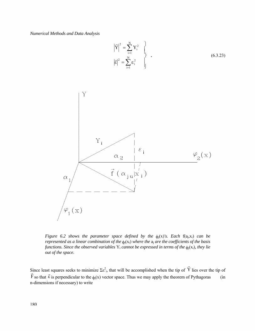
Figure 6.2 shows the parameter space defined by the φj(x)'s. Each f(aj,xi) can be
represented as a linear combination of the φj(xi) where the aj are the coefficients of the basis functions. Since the observed variables Yi cannot be expressed in terms of the φj(xi), they lie out of the space.
Since least squares seeks to minimize Σε2
i, that will be accomplished when the tip of Yr
lies over the tip of Fr
so that is perpendicular to the φεr
j(x) vector space. Thus we may apply the theorem of Pythagoras (in n-dimensions if necessary) to write
180
6 - Least Squares
∑ ∑ ∑= = =
−=εN
1i
N
1i
N
1iij
2i
2ii
2ii )x,a(fwYww . (6.3.24)
Here we have included the square weights wi as their inclusion in no way changes the result. From the definition of the mean square residual we have
∑ ∑ ∑∑∑= = ===
+−=−=εN
1i
N
1i
N
1iij
2i
N
1iijii
N
1i
2ii
2ijii
2ii )x,a(fw)x,a(fYw2Yw)]x,a(fY[w)w( , (6.3.25)
which if we combine with equation (6.3.24) will allow us to eliminate the quadratic term in f2 so that equation (6.3.21) finally becomes
⎟⎟⎠
⎞⎜⎜⎝
⎛⎥⎦
⎤⎢⎣
⎡φ−⎥
⎦
⎤⎢⎣
⎡⎥⎦
⎤⎢⎣
⎡−
=δ ∑ ∑∑= ==
n
0k
N
1iikiik
N
1i
2ii
jj2j )x(YwaYw
nNC
)a( . (6.3.26)
The term in the square brackets on the far right hand side is the constant vector of the normal equations. Then the only unknown term in the expression for δaj is the scalar term [ΣwiYi
2], which can easily be generated during the formation of the normal equations. Thus it is possible to estimate the effect of errors in the data on the solution set of least square coefficients using nothing more than the constant vector of the normal equations, the diagonal elements of the inverse matrix of the normal equations, the solution itself, and the weighted sum squares of the dependent variables. This amounts to a trivial calculation compared to the solution of the initial problem and should be part of any general least square program. d. The Effects of Errors in the Independent Variable Throughout the discussion in this section we have investigated the effects of errors in the dependent variable. We have assumed that there is no error in the independent variable. Indeed the least square norm itself makes that assumption. The "best" solution in the least square sense is that which minimizes the sum square of the residuals. Knowledge of the independent variable is assumed to be precise. If this is not true, then real problems emerge for the least square algorithm. The general problem of uncorrelated and unknown errors in both x and Y has never been solved. There do exist algorithms that deal with the problem where the ratio of the errors in Y to those in x is known to be a constant. They basically involve a coordinate rotation through an angle α = tan(x/y) followed by the regular analysis. If the approximating function is particularly simple (e.g. a straight line), it may be possible to invert the defining equation and solve the problem with the role of independent and dependent variable interchanged. If the solution is the same (allowing for the transformation of variables) within the formal errors of the solution, then some confidence may be gained that a meaningful solution has been found. Should they differ by more than the formal error then the analysis is inappropriate and no weight should be attached to the solution. Unfortunately, inversion of all but the simplest problems will generally result in a non-linear system of equations if the inversion can be found at all. So in the next section we will discuss how one can approach a least square problem where the normal equations are non-linear.
181
Numerical Methods and Data Analysis
6.4 Non-linear Least Squares In general, the problem of non-linear least squares is fraught with all the complications to be found with any non-linear problem. One must be concerned with the uniqueness of the solution and the non-linear propagation of errors. Both of these basic problems can cause great difficulty with any solution. The simplest approach to the problem is to use the definition of least squares to generate the normal equations so that
n,,1,0j,0a
)x,a(f)]x,a(fY[w
N
1i j
ijijii L==
∂
∂−∑
= . (6.4.1)
These n+1 non-linear equations must then be solved by whatever means one can find for the solution of non-linear systems of equations. Usually some sort of fixed-point iteration scheme, such as Newton-Raphson, is used. However, the error analysis may become as big a problem as the initial least square problem itself. Only when the basic equations of condition will give rise to stable equations should the direct method be tried. Since one will probably have to resort to iterative schemes at some point in the solution, a far more common approach is to linearize the non-linear equations of condition and solve them iteratively. This is generally accomplished by linearizing the equations in the vicinity of the answer and then solving the linear equations for a solution that is closer to the answer. The process is repeated until a sufficiently accurate solution is achieved. This can be viewed as a special case of a fixed-point iteration scheme where one is required to be relatively near the solution. In order to find appropriate starting values it is useful to understand precisely what we are trying to accomplish. Let us regard the sum square of the residuals as a function of the regression coefficients aj so that
∑∑==
χ=ε=−N
1ij
22ii
N
1i
2ijii )a(w)]x,a(fY[w . (6.4.2)
For the moment, we shall use the short hand notation of χ2 to represent the sum square of the residuals. While the function f(aj,x) is no longer linear in the aj's they may be still regarded as independent and therefore can serve to define a space in which χ2 is defined. Our non-linear least square problem can be geometrically interpreted to be finding the minimum in the χ2 hypersurface (see figure 6.2). If one has no prior knowledge of the location of the minima of the χ2 surface, it is best to search the space with a coarse multidimensional grid. If the number of variables aj is large, this can be a costly search, for if one picks m values of each variable aj, one has mn functional evaluations of equation (6.4.2) to make. Such a search may not locate all the minima and it is unlikely to definitively locate the deepest and therefore most desirable minimum. However, it should identify a set(s) of parameters from which one of the following schemes will find the true minimum.
0ka
We will consider two basic approaches to the problem of locating these minima. There are others, but they are either logically equivalent to those given here or very closely related to them. Basically we shall assume that we are near the true minimum so that first order changes to the solution set ak
0 will lead us to that minimum. The primary differences in the methods are the manner by which the equations are formulated.
182
6 - Least Squares
a. The Method of Steepest Descent A reasonable way to approach the problem of finding a minimum in χ2-space would be to change the values of aj so that one is moving in the direction, which yields the largest change in the value of χ2. This will occur in the direction of the gradient of the surface so that
⎪⎪
⎭
⎪⎪
⎬
⎫
∆
χ−∆+χ=
∂χ∂
∂χ∂
=χ∇ ∑=
j
0j
2j
0j
2
j
2
N
1ij
j
22
a)a()aa(
a
aa
. (6.4.3)
We can calculate this by making small changes ∆aj in the parameters and evaluating the components of the gradient in accordance with the second of equations (6.4.3). Alternately, we can use the definition of least squares and calculate
∑= ∂
∂−=
∂χ∂
=χ∇N
1i j
ijijii
j
22
j a)x,a(f
)]x,a(fY[w2a
. (6.4.4)
If the function f(aj,x) is not too complicated and has closed form derivatives, this is by far the preferable manner to obtain the components of ∇χ2. However, we must exercise some care as the components of ∇χ2 are not dimensionless. In general, one should formulate a numerical problem so that the units don't get in the way. This means normalizing the components of the gradient in some fashion. For example we could define
∑∑==
χ∇
χ∇=
χχ∇
χχ∇=ξ n
0j
2jj
2jj
n
0j
22jj
22jj
i
a
a
/a
]/a[ , (6.4.5)
which is a sort of normalized gradient with unit magnitude. The next problem is how far to apply the gradient in obtaining the next guess, A conservative possibility is to use ∆aj from equation (6.4.3) so that
δaj = ∆aj/ξj . (6.4.6) In order to minimize computational time, the direction of the gradient is usually maintained until χ2 begins to increase. Then it is time to re-evaluate the gradient. One of the difficulties of the method of steepest descent is that the values of the gradient of χ2 vanish as one approaches a minimum. Therefore the method becomes unstable as one approaches the answer in the same manner and for the same reasons that Newton-Raphson fixed-point iteration became unstable in the vicinity of multiple roots. Thus we shall have to find another approach.
183
Numerical Methods and Data Analysis
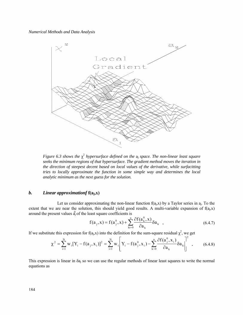
Figure 6.3 shows the χ2 hypersurface defined on the aj space. The non-linear least square
seeks the minimum regions of that hypersurface. The gradient method moves the iteration in the direction of steepest decent based on local values of the derivative, while surfacitting tries to locally approximate the function in some simple way and determines the local analytic minimum as the next guess for the solution.
b. Linear approximationf f(aj,x) Let us consider approximating the non-linear function f(aj,x) by a Taylor series in aj. To the extent that we are near the solution, this should yield good results. A multi-variable expansion of f(aj,x) around the present values aj
0 of the least square coefficients is
∑=
δ∂
∂+=
n
0kik
k
0k0
jj aa
)x,a(f)x,a(f)x,a(f . (6.4.7)
If we substitute this expression for f(aj,x) into the definition for the sum-square residual χ2, we get
∑ ∑ ∑= = = ⎥
⎥⎦
⎤
⎢⎢⎣
⎡δ
∂
∂−−=−=χ
N
1i
N
1i
2n
0kk
k
i0j
i0jii
2ijii
2 aa
)x,a(f)x,a(fYw)]x,a(fY[w . (6.4.8)
This expression is linear in δaj so we can use the regular methods of linear least squares to write the normal equations as
184
6 - Least Squares
n,,1,0p,0a
)x,a(fa
a)x,a(f
)x,a(fYw2a
N
1i p
i0j
n
0kk
k
i0j
i0jii
p
2
L==∂
∂
⎥⎥⎦
⎤
⎢⎢⎣
⎡δ
∂
∂−−=
δ∂χ∂ ∑ ∑
= = , (6.4.9)
which can be put in the standard form of a set of linear algebraic equations for δak so that
⎪⎪⎪⎪
⎭
⎪⎪⎪⎪
⎬
⎫
=∂
∂−=
==∂
∂
∂
∂=
==δ
∑
∑
∑
=
=
=
N
1i p
i0j
i0jiip
N
1i p
i0j
k
i0j
ikp
n
0kpkpk
n,,1,0p,a
)x,a(f)]x,a(fY[wB
n,,1,0p,n,,1,0k,a
)x,a(fa
)x,a(fwA
n,,1,0p,BAa
L
LL
L
. (6.4.10)
The derivative of f(aj,x) that appears in equations (6.4.9) and (6.4.10) can either be found analytically or numerically by finite differences where
p
i0p
0jip
0p
0j
p
ij
a)x,a,a(f]x),aa(,a[f
a)x,a(f
∆
−∆+=
∂
∂ . (6.4.11)
While the equations (6.4.10) are linear in δak, they can be viewed as being quadratic in ak. Consider any expansion of ak in terms of χ2 such as
ak = q0 + q1χ2 + q2χ4 . (6.4.12) The variation of ak will then have the form
δak = q1 + 2q2χ2 , (6.4.13) which is clearly linear in χ2. This result therefore represents a parabolic fit to the hypersurface χ2 with the condition that δak is zero at the minimum value of χ2. The solution of equations (6.4.10) provides the location of the minimum of the χ2 hypersurface to the extent that the minimum can locally be well approximated by a parabolic hypersurface. This will certainly be the case when we are near the solution which is precisely where the method of steepest descent fails. It is worth noting that the constant vector of the normal equations is just half of the components of the gradient given in equation (6.4.4). Thus it seems reasonable that we could combine this approach with the method of steepest descent. One approach to this is given by Marquardt4. Since we were somewhat arbitrary about the distance we would follow the gradient in a single step we could modify the diagonal elements of equations (6.4.10) so that
⎭⎬⎫
≠==λ+=
pk,A'An,,1,0k,)1(A'A
kpkp
kkkk L . (6.4.14)
Clearly as λ increases, the solution approaches the method of steepest descent since
Lim δak = Bk/λAkk . (6.4.15) λ→∞
185
Numerical Methods and Data Analysis
All that remains is to find an algorithm for choosing λ. For small values of λ, the method approaches the first order method for δak. Therefore we will choose λ small (say about 10-3) so that the δak's are given by the solution to equations (6.4.10). We can use that solution to re-compute χ2. If
)a()aa( 22 rrrχ>δ+χ , (6.4.16)
then increase λ by a factor of 10 and repeat the step. However, if condition (6.4.16) fails and the value of χ2 is decreasing, then decrease λ by a factor of 10, adopt the new values of ak and continue. This allows the analytic fitting procedure to be employed where it works the best - near the solution, and utilizes the method of steepest descent where it will give a more reliable answer - well away from the minimum. We still must determine the accuracy of our solution. c. Errors of the Least Squares Coefficients The error analysis for the non-linear case turns out to be incredibly simple. True, we will have to make some additional assumptions to those we made in section 6.3, but they are reasonable assumptions. First, we must assume that we have reached a minimum. Sometimes it is not clear what constitutes a minimum. For example, if the minimum in χ2 hyperspace is described by a valley of uniform depth, then the solution is not unique, as a wide range of one variable will minimize χ2. The error in this variable is large and equal at least to the length of the valley. While the method we are suggesting will give reliable answers to the formal errors for aj when the approximation accurately matches the χ2 hypersurface, when it does not the errors will be unreliable. The error estimate relies on the linearity of the approximating function in δaj. In the vicinity of the χ2 minimum
δaj = aj ─ aj 0 . (6.4.17)
For the purposes of the linear least squares solution that produces δaj, the initial value aj
0 is a constant devoid of any error. Thus when we arrive at the correct solution, the error estimates for δaj will provide the estimate for the error in aj itself since
∆(δaj) = ∆aj ─ ∆[aj 0] = ∆aj . 6.4.18)
Thus the error analysis we developed for linear least squares in section 6.3 will apply here to finding the error estimates for δaj and hence for aj itself. This is one of the virtues of iterative approaches. All past sins are forgotten at the end of each iteration. Any iteration scheme that converges to a fixed-point is in some real sense a good one. To the extent that the approximating function at the last step is an accurate representation of the χ2 hypersurface, the error analysis of the linear least squares is equivalent to doing a first order perturbation analysis about the solution for the purposes of estimating the errors in the coefficients representing the coordinates of the hyperspace function. As we saw in section 6.3, we can carry out that error analysis for almost no additional computing cost. One should keep in mind all the caveats that apply to the error estimates for non-linear least squares. They are accurate only as long as the approximating function fits the hyperspace. The error distribution of the independent variable is assumed to be anti-symmetric. In the event that all the conditions are met, the errors are just what are known as the formal errors and should be taken to represent the minimum errors of the parameters.
186
6 - Least Squares
6.5 Other Approximation Norms Up to this point we have used the Legendre Principle of Least Squares to approximate or "fit" our data points. As long as this dealt with experimental data or other forms of data which contained intrinsic errors, one could justify the Least Square norm on statistical grounds (as long as the error distribution met certain criteria). However, consider the situation where one desires a computer algorithm to generate, say, sin(x) over some range of x such as 0xπ/4. If one can manage this, then from multiple angle formulae, it is possible to generate sin(x) for any value of x. Since at a very basic level, digital computers only carry out arithmetic, one would need to find some approximating function that can be computed arithmetically to represent the function sin(x) accurately over that interval. A criterion that required the average error of computation to be less than ε is not acceptable. Instead, one would like to be able to guarantee that the computational error would always be less than εmax. An approximating norm that will accomplish this is known as the Chebyschev norm and is sometimes called the "mini-max" norm. Let us define the maximum value of a function h(x) over some range of x to be
hmax ≡Max│h(x)│ ∀ allowed x . (6.5.1) Now assume that we have a function Y(x) which we wish to approximate by f(aj,x) where aj represents a set of free parameters that may be adjusted to provide the "best" approximation in some sense. Let h(x) be the difference between those two functions so that
h(x) = ε(x) = Y(x) ─ f(aj,x) . (6.5.2) The least square approximation norm would say that the "best" set of aj's is found from
Min ∫ ε2(x)dx . (6.5.3)
However, an approximating function that will be the best function for computational approximation will be better given by
Min│hmax│ = Min│ε max│ = Min│Max│Y(x)-f(aj,x)││. (6.5.4) A set of adjustable parameters aj that are obtained by applying this norm will guarantee that
ε(x) ≤ εmax ∀x , (6.5.5) and that εmax is the smallest possible value that can be found for the given function f(aj,x). This guarantees the investigator that any numerical evaluation of f(x) will represent Y(x) within an amount εmax. Thus, by minimizing the maximum error, one has obtained an approximation algorithm of known accuracy throughout the entire range. Therefore this is the approximation norm used by those who generate high quality functional subroutines for computers. Rational functions are usually employed for such computer algorithms instead of ordinary polynomials. However, the detailed implementation of the norm for determining the free parameters in approximating rational functions is well beyond the scope of this book. Since we have emphasized polynomial approximation throughout this book, we will discuss the implementation of this norm with polynomials.
187
Numerical Methods and Data Analysis
a. The Chebyschev Norm and Polynomial Approximation Let our approximating function f(aj,x) be of the form given by equation (3.1.1) so that
∑=
φ=n
0jjjj )x(a)x,a(f . (6.5.6)
The choice of f(aj,x) to be a polynomial means that the free parameters aj will appear linearly in any analysis. So as to facilitate comparison with our earlier approaches to polynomial approximation and least squares, let us choose φj to be xj and we will attempt to minimize εmax(x) over a discrete set of points xi. Thus we wish to find a set of aj so that
xxaYMin)(Minmax
n
0j
ijjimaxi ∀−=ε ∑
= . (6.5.7)
Since we have (n+1) free parameters, aj, we will need at least N = n+1 points in our discrete set xi. Indeed, if n+1 = N then we can fit the data exactly so that εmax will be zero and the aj's could be found by any of the methods in chapter 3. Consider the more interesting case where N >> n+1. For the purposes of an example let us consider the cases where n = 0, and 1 . For n = 0 the approximating function is a constant, represented by a horizontal line in figure 6.4
Figure 6.4 shows the Chebyschev fit to a finite set of data points. In panel a the fit is with a
constant a0 while in panel b the fit is with a straight line of the form f(x) = a1x+a0. In both cases, the adjustment of the parameters of the function can only produce (n+2) maximum errors for the (n+1) free parameters.
By adjusting the horizontal line up or down in figure 6.3a we will be able to get two points to have the same largest value of │εi│ with one change in sign between them. For the straight line in Figure 6.3b, we will be able to adjust both the slope and intercept of the line thereby making the three largest values of │εi│ the same. Among the extreme values of εi there will be at least two changes in sign. In general, as long as N > (n+1), one can adjust the parameters aj so that there are n+2 extreme values of εi all equal to εmax and there will be (n+1) changes of sign along the approximating function. In addition, it can be shown that the aj's will be unique. All that remains is to find them.
188
6 - Least Squares
b. The Chebyschev Norm, Linear Programming, and the Simplex
Method Let us begin our search for the "best" set of free-parameters aj by considering an example. Since we will try to show graphically the constraints of the problem, consider an approximating function of the first degree which is to approximate three points (see figure 6.3b). We then desire
⎪⎪⎭
⎪⎪⎬
⎫
ε=ε
ε≤+−ε≤+−ε≤+−
maxmax
max3103
max2102
max1101
Min)xaa(Y)xaa(Y)xaa(Y
. (6.5.8)
Figure 6.5 shows the parameter space for fitting three points with a straight line under the
Chebyschev norm. The equations of condition denote half-planes which satisfy the constraint for one particular point.
These constraints constitute the basic minimum requirements of the problem. If they were to be plotted in parameter space (see Figure 6.4), they would constitute semi-planes bounded by the line for ε = 0. The half of the semi-plane that is permitted would be determined by the sign of ε. However, we have used the result from above that there will be three extreme values for εi all equal to εmax and having opposite sign. Since the value of εmax is unknown and the equation (in general) to which it is attached is also unknown, let us regard it as a variable to be optimized as well. The semi-planes representing the constraints are now extended out of
189
Numerical Methods and Data Analysis
the a0-a1 plane in the direction of increasing│εmax│ with the semi-planes of the constraints forming an inverted irregular pyramid. The variation of the sign of εmax guarantees that the planes will intersect to form a convex solid. The solution to our problem is trivial, as the lower vertex of the pyramid represents the minimum value of the maximum error, which will be the same for each constraint. However, it is nice that the method will tell us that without it being included in the specification of the problem. Since the number of extrema for this problem is 1+2, this is an expected result. The inclusion of a new point produces an additional semi-constraint plane which will intersect the pyramid producing a triangular upper base. The minimum value of the maximum error will be found at one of the vertices of this triangle. However since the vertex will be defined by the intersection of three lines, there will still be three extrema as is required by the degree of the approximating polynomial. Additional points will increase the number of sides as they will cut the initial pyramid forming a multi-sided polygon. The vertices of the polygon that is defined in parameter-εmax space will still hold the optimal solution. In this instance the search is simple as we simply wish to know which εmax is the smallest in magnitude. Thus we look for the vertex nearest the plane of the parameters. An increase in the number of unknowns ai's will produce figures in higher dimensions, but the analysis remains essentially the same. The area of mathematics that deals with problems that can be formulated in term of linear constraints (including inequalities) is known as Linear Programming and it has nothing to do with computer programming. It was the outgrowth of a group of mathematicians working in a broader area of mathematics known as operations research. The inspiration for its development was the finding of solutions to certain optimization problems such as the efficient allocation of scarce resources (see Bland4). Like many of the subjects we have introduced in this book, linear programming is a large field of study having many ramifications far beyond the scope of this book. However, a problem that is formulated in terms of constraint inequalities will consist of a collection of semi-spaces that define a polytope (a figure where each side is a polygon) in multidimensional parameter space. It can be shown that the optimum solution lies at one of the vertices of the polytope. A method for sequentially testing each vertex so that the optimal one will be found in a deterministic way is known as the simplex method. Starting at an arbitrary vertex one investigates the adjacent vertices finding the one which best satisfies the optimal conditions. The remaining vertices are ignored and one moves to the new "optimal" vertex and repeats the process. When one can find no adjacent vertices that better satisfy the optimal condition that vertex is the most optimal of the entire polytope and represents the optimal solution to the problem. In practice, the simplex method has been found to be far more efficient than general theoretical considerations would lead one to expect. So, while there are other approaches to linear programming problems, the one that still attracts most attention is the simplex method. c. The Chebyschev Norm and Least Squares At the beginning of this chapter, we justified the choice of the Least Square approximation norm on the grounds that it yielded linear equations of condition and was the lowest power of the deviation ε that was guaranteed to be positive. What about higher powers? The desire to keep the error constraints positive should limit us to even powers of ε. Thus consider a norm of the form
Min Σ εi 2n = Min Σ [Yi-f(aj,xi)]2n , (6.5.9)
i i
190
6 - Least Squares
which lead to the non-linear equations
[ ] [ ] 0a
)x,a(f)x,a(fyn2)x,a(fy
a j
ij1n2iji
ii
n2iji
j
=∂
∂−=⎟
⎠
⎞⎜⎝
⎛−
∂∂ −∑∑ . (6.5.10)
Now one could solve these non-linear equations, but there is no reason to expect that the solution would be "better" in any real sense than the least square solution. However, consider the limit of equation (6.5.9) as n→∞.
Lim( Min Σ εi 2n ) = Min( Lim Σ εi
2n ) = Min│εmax│2n . (6.5.11) n→∞ i n→∞ i
The solution that is found subject to the constraint that ε2nmax is a minimum will be the same solution that is
obtained when εmax is a minimum. Thus the limit of the 2nth norm as n goes to infinity is the Chebyschev norm. In this chapter we have made a transition from discussing numerical analysis where the basic inputs to a problem are known with arbitrary accuracy tp those where the basic data contained errors. In earlier chapters the only errors that occur in the calculation result from round-off of arithmetic processes or truncation of the approximation formulae. However, in section 6.3 we allowed for the introduction of "flawed" inputs, with inherent errors resulting from experiment or observation. Since any interaction with the real world will involve errors of observation, we shall spend most of the remainder of the book discussing the implication of these errors and the manner by which they can be managed.
191
Numerical Methods and Data Analysis
Chapter 6 Exercises 1. Develop normal equations for the functions: a. f(x) = a0e a 1 x b. f(x) = a0 + a1sin(a2πx + a3) . Which expressions could be replaced with a linear function with no loss of accuracy? What would
the error analysis of that function fit to observational data say about the errors of the original coefficients aj?
2. Using least squares find the "best" straight-line fit and the error estimates for the slope and intercept
of that line for the following set of data. xi Yi
1 1.5 2 2.0 3 2.8 4 4.1 5 4.9 6 6.3 7 5.0 8 11.5 3. Fit the following table with a polynomial of the form f(aj,x) = Σ
k φk(x), where φk(x) = cos(kπx)
xi f(aj,xi) 0.00000 0.00000 0.17453 0.17101 0.34907 0.32139 0.41888 0.37157 0.62839 0.47553 0.78540 0.49970 1.0123 0.44940 1.0821 0.41452 1.2915 0.26496 1.5010 0.06959 How many terms are required to fit the table accurately? Discuss what you mean by "accurately"
and why you have chosen that meaning.
192
6 - Least Squares
4. Given the following two sets of data to be fit by straight lines. x1,i Y1,i x2,i Y2,i
1 9.1 1 0.5 2 8.5 2 3.2 3 7.6 3 2.5 4 3.5 4 4.6 5 4.2 5 5.1 6 2.1 6 6.9 7 0.2 7 6.8 find the "best" value for the intersection of the straight lines and an estimate for the error in Y. How
would you confirm the assumption that there is no error in x? 5. Determine the complex Fourier transform of
a. e-t2 -∞ < t < +∞.
b. e-tcos(t) , 0 < t < +∞ . 6. Find the FFT for the functions in problem 5 where the function is sampled every .01 in t and the
total number of points is 1024. Calculate the inverse transform of the result and compare the accuracy of the process.
193
Numerical Methods and Data Analysis
Chapter 6 References and Supplementary Reading 1. Bateman, H., "Tables of Integral Transforms" (1954) Ed. A.
Erde'lyi, Volumes 1,2, McGraw-Hill Book Co., Inc. New York, Toronto, London. 2. Press, W.H., Flannery, B.P., Teukolsky, S.A., and Vetterling, W.T., "Numerical Recipies the Art
of Scientific Computing" (1986), Cambridge University Press, Cambridge, pp. 390-394. 3. Marquardt, D.W., "An Algorithm for Least-Squares Estimation of Nonlinear Parameters", (1963),
J. Soc. Ind. Appl. Math., Vol.11, No. 2, pp.431-441. 4. Bland, R.G., "The Allocation of Resources by Linear Programming", (1981) Sci. Amer. Vol. 244,
#6, pp.126-144. Most books on numerical analysis contain some reference to least squares. Indeed most freshmen calculus courses deal with the subject at some level. Unfortunately no single text contains a detailed description of the subject and its ramifications. 1. Hildebrand, F.B., "Introduction to Numerical Analysis" (1956) McGraw-Hill Book Co., Inc.,
New York, Toronto, London, pp. 258-311, This book presents a classical discussion and much of my discussion in section 6.3 is based on his presentation. The error analysis for non-linear least squares in section 6.4 is dealt with in considerable detail in 2. Bevington, P.R., "Data Reduction and Error Analysis for the Physical Sciences", (1969),
McGraw-Hill Book Co. Inc., New York, San Francisco, St. Louis, Toronto, London, Sydney, pp. 204-246.
Nearly any book that discusses Fourier series and transforms contains useful information elaborating on the uses and extended theory of the subject. An example would be 3. Sokolnikoff, I.S., and Redheffer, R.M., "Mathematics of Physics and Modern Engineering",
(1958) McGraw-Hill Book Co., Inc. New York, Toronto, London, pp. 175-211. Two books completely devoted to Fourier analysis and the transforms particularly are: 4. Brigham, E.O., "The Fast Fourier Transform", (1974) Prentice-Hall, Inc. Englewood Cliffs, N.J., and 5. Bracewell, R.N., "The Fourier Transform and its Applications", 2nd Ed., (1978),
McGraw-Hill Book Company, New York N.Y.
194
6 - Least Squares
A very compressed discussion, of Linear Programming, which covers much more that we can, is to be found in 6. Press, W.H., Flannery, B.P., Teukolsky, S.A., and Vetterling, W.T., "Numerical Recipies the Art
of Scientific Computing" (1986), Cambridge University Press, Cambridge. pp. 274-334, but a more basic discussion is given by