6. THE HORROCKS LEGACY

6.1 INTRODUCTION

During 1752 a major change took place in Mayer’s thinking about modelling of themoon’s motion, affecting the procedure to be followed when computing a lunar po-sition from the tables. Initially the tables were applied in the single-stepped fashion(using the terminology explained in section 3.5), but during 1752 Mayer switched toa multistepped procedure. He would basically adhere to the multistepped procedureever after, changing only some of the details later on.

The purpose of the present chapter is to investigate the origin of this multi-stepped procedure. I will show that Mayer developed it out of a lunar theory ofNewton’s, which first appeared in print in 1702. This dependence of Mayer’s tableson Newton’s 1702 lunar theory, which at best has a very troublesome relation to thetheory of gravitation, has never been noted before. On the contrary, it is usuallysaid that Mayer’s tables were in some way based on Euler’s lunar theory, and thattheir advent made those founded on Newton’s 1702 lunar theory obsolete.1 It willhere be shown that Newton’s theory has exercised, through Mayer’s tables, a muchmore profound impact on 18th century positional astronomy than has hitherto beenthought.

We will see in the next chapter how to transform any multistepped scheme intoa single-stepped scheme that is equivalent for all practical purposes, The implica-tion is that none of the possible schemes has a real advantage over any other asfar as achievable accuracy is concerned. Nonetheless Mayer attained a most strik-ing improvement in accuracy as soon as he adopted the multistep procedure. Themanuscripts that witness the emergence of his new scheme suggest that he was atthat time unable to provide a complete and coherent lunar theory to back up hisnew tables. The development of the multistepped scheme happened apparently forpragmatic rather than theoretical reasons, and it is highly unlikely that Mayer had avalid theoretical justification for the multistep over the single-step procedure.

The influence of Newton’s lunar theory on Mayer provides yet another argu-ment against the commonly held belief that Mayer’s tables are merely Euler’s equa-tions (either in the astronomical or the mathematical sense) with their coefficients

1 The relation between Mayer’s and Euler’s lunar theories has been discussed in the previouschapter. Statements effectively equivalent to ‘Newton out, Mayer in’ can be found in e.g.,[Wilson and Taton, 1989, p. 162], [Kollerstrom, 2000, pp. 233–4], [Whiteside, 1976, p. 324].Petrus Frisius came very close to recognizing Mayer’s dependence on Newton’s lunar theory,only to conclude that Mayer had fitted Euler’s theory to observations , [Frisius, 1768, pp. 272–3,357].

6.2. Newton on lunar motion, 1702 85

adjusted to observations: that belief leaves the multistep procedure unexplained.We also see the role of the calculus in the development of Mayer’s 1753 kil tablesreduced to a subsidiary one, at most. But a final judgement of the relative mer-its of the calculus, Newton’s theory, and observations is more delicate and will bepostponed until the final chapter.

The current chapter is organized as follows. In section 6.2 we will start with astudy of the 1702 ‘theory’ of Isaac Newton, which is, as we will see, rather a set ofrules to construct lunar tables than a theory in the modern sense of the word. Thoserules are presented in section 6.3. Then follow two sections on a crucial ingredientof Newton’s lunar theory that had developed out of an idea of Jeremiah Horrocks(1618–1641): a variable eccentricity and direction of the apsidal line of the lunarorbit. The kinematics of Horrocks’s idea is explained in section 6.4, and in 6.5 it istranslated into the language of trigonometric functions. The results will go slightlybeyond what has already been published on the subject.

Section 6.6 is devoted to the lunar tables of Pierre Charles Lemonnier. His ta-bles were probably the widest available implementation of Newton’s prescriptions,and they were instrumental in the transmission of Newton’s rules to Mayer. Mayer’sassimilation of the Newtonian Lemonnier tables is the subject of section 6.7, wherewe study the relevant manuscripts. It will become clear that Mayer’s interest inNewton’s theory arose when he was apparently in doubt of how to proceed furtherin lunar theory.

Then follows an investigation of the measure of success of some of Mayer’stable versions. In particular, we compare the accuracy of his tables before and afterthe multistep reform. The accuracy of Lemonnier’s tables is included too. We willdiscover that the tables based on a multistepped scheme result in higher accuracythan Mayer’s initial single-stepped scheme. Some insight will also be gained in thefurther improvements that Mayer attained. Finally, will be looked upon with fresheyes we will take a look at Mayer’s own preface to his printed tables.

6.2 NEWTON ON LUNAR MOTION, 1702

In 1702 Isaac Newton’s Theory of the Moon’s Motion (NTM) appeared, a pamphletcontaining a set of rules for the production of tables for the computation of theposition of the moon. Four nearly identical editions, three in English and one inLatin, have appeared of that text; the Latin version was first published in DavidGregory’s Astronomiae Physicae & Geometricae Elementa, 1702. All four havebeen reproduced in facsimile with a general introduction by I. Bernard Cohen.2

2 [Newton, 1975]. Cohen makes a distinction between (i) the 1702 pamphlet, (ii) its contentswithout reference to a specific edition, and (iii) Newton’s work on lunar theory in general.The abbreviation NTM for Newton’s Theory of the Moon is in line with Cohen’s indicationof the second category. An impression of Newton’s work on lunar theory is provided in[Whiteside, 1976]; also see A guide to Newton’s Principia, in [Newton et al., 1999], particu-larly §8.14, The Motion of the Moon, by I. B. Cohen, and §8.15, Newton and the Problem of theMoon’s Motion, by George E. Smith. [Kollerstrom, 2000] discusses the procedures of NTM,

86 6. The Horrocks Legacy

NTM is not a theory as one might perhaps expect. In fact, quite different fromthe modern scientific idea of a theory, lunar theory in that time denoted, in thewords of Francis Baily, ‘rules or formulae for constructing diagrams and tables thatwould represent the celestial motions and observations with accuracy’.3 Nothingelse could have been expected before the formulation of a causal physical theory ofmovement of celestial bodies. Even after he had provided precisely such a physicaltheory, Newton continued to use the word in its traditional sense.

The first edition of Newton’s Principia, of 1687, contained a significantly morerudimentary lunar theory than the 1702 pamphlet. Somewhat modified and con-densed forms of the NTM prescriptions found their way into the second (1713) andthird (1726) editions of the Principia, where they can be found in the Scholium toProposition 35, Book III, following a quantitative examination (ignoring eccentric-ity) of the variability of the inclination of the lunar orbit, the motion of the nodes,and the variation. In addition, Proposition 25 of Book III called upon the manycorollaries of Proposition 66 of Book I for a qualitative explanation of all knownlunar equAtions, and some new ones.4

A very characteristic feature of NTM, which we will discuss at length in the fol-lowing two sections, was adapted from an older, kinematic, lunar theory of JeremiahHorrocks. This suggests that Newton’s lunar theory was a mix of his own dynamicalresearch and of Horrocks’s kinematic model.

Surprisingly, gravitation was only mentioned once in NTM, and then only in thepreface, perhaps written by Halley:

This Irregularity of the Moon’s Motion depends (as is now well known, since Mr. Newton hathdemonstrated the Law of Universal Gravitation) on the Attraction of the Sun, which perturbsthe Motion of the Moon [. . . ]. But this being now to be accounted for, and reduced to a Rule;by this Theory such Allowances are made for it, as that the Place of the Planet shall be trulyEquated.5

The text ascribes the cause of the perturbations to the attraction of the sun, andstresses that it is now time to lay down rules to compute the perturbed motion ofthe moon, but it avoids to aver that the rules are purely deduced from the law ofgravitation. Indeed, the main text of NTM supplied these rules, as a true theory inthe pre-Newtonian sense of that word.

In Principia however, Newton repeatedly averred that he had obtained all hisresults from application of the law of gravitation to the Sun-Earth-Moon system,

assesses its accuracy using computer simulations, and points to various places where NTM wasused in the 18th century, missing—like every other researcher before him—its influence onMayer. [Cook, 2000] contains a well-balanced and illuminating view of Newton’s work onlunar motion, providing physical insight while avoiding mathematical detail.

3 [Baily, 1835, p. 690], quoted in [Newton, 1975, p. 3]. The on-line edition of the Merriam-Webster dictionary (http://www.m-w.com) defines theory as ‘a plausible or scientifically ac-ceptable general principle or body of principles offered to explain phenomena’. Indeed, noteverything that Newton wrote was Newtonian!

4 The notorious attempt in Book I Proposition 45 on the mean motion of the apsidal line is of noconcern to us now; see [Waff, 1975] for that.

5 [Newton, 1975, pp. 94–95]. Cohen discusses the allusion to Halley on pp. 31–32.

6.3. The equations of NTM 87

but he omitted his derivations in all but the above-mentioned three cases: varia-tion, nodal movement, and inclination. Michael Nauenberg has pointed to certainmanuscripts in the Portsmouth collection where Newton apparently applied a per-turbation technique that might have allowed him to obtain the results of NTM.6

Nauenberg’s point of view that Newton indeed had provided a dynamical and grav-itational basis for the Horrocksian part of his theory is not accepted by everybody.Probably, though, Newton was able to obtain the form of some equAtions of lu-nar motion theoretically, whereafter he adjusted the coefficients to observations; atleast, he explained to Flamsteed that this was his procedure. Although some of theequAtions were new discoveries disclosed by the law of gravitation, Whiteside andKollerstrom maintain that Newton went back to the Horrocksian model in despair,after failing to account for all the lunar equAtions by gravitation.7 It is of interestthat Newton adapted a similar model in an attempt on the Jupiter-Saturn inequAlity,as Wilson noted.8

Surely, the moon had played a crucial role in Newton’s discovery of the lawof gravitation; yet the intricacies of lunar motion made his head ache, as New-ton confessed to Machin. Although we regard Newton also as an inventor of thedifferential- and integral calculus, the tools at Newton’s disposal were quite differ-ent from the tools that were developed later in the 18th century. Wilson explained itlucidly thus:

Newton worked out the motions of celestial bodies while thinking predominantly geometrically,and at every step he had to give full account of the dynamics of the problem. In the eighteenth-century approaches, differential equations were formed on geometrical and dynamical grounds,whereafter the solution lay in the realm of analysis, having to find successive approximationsto an analytical function.9

It is safe to say that the theoretical basis of NTM is still unclear today.10

6.3 THE EQUATIONS OF NTM

NTM first specified the epochs and mean motions of the lunar longitude, apogee,and node, and the solar longitude and apogee, and then proceeded to describe theseveral equAtions. We will now have a more detailed look at these equAtions, rep-resenting them in modern, analytical form.11 We will need the amount of detailincluded here in this section to appreciate the impact of NTM on Mayer later on inthe chapter.

6 For pointers, see [Nauenberg, 1998], [Nauenberg, 2000], [Nauenberg, 2001].7 [Whiteside, 1976], [Kollerstrom, 2000].8 [Wilson, 1985, p. 17].9 [Wilson, 2001, p. 178]; also see [Wilson, 1985, p. 69+]10 [Baily, 1835, pp. 139–140], [Newton, 1975, p. 39], [Whiteside, 1976], [Wilson, 1995a, p. 50],

[Kollerstrom, 2000]. The source of the anecdote of Newton’s headache is a notebook of JohnConduitt [Whiteside, 1976, p. 324].

11 The research is based mainly on Cohen’s edition of NTM [Newton, 1975, pp. 91–119], with[Kollerstrom, 2000] as a secondary source.

88 6. The Horrocks Legacy

NTM’s procedure is of the kind where each equAtion affects the argumentsbefore the next equAtion is computed: it can be regarded as a multistep procedurewith only one equAtion per step. NTM has seven steps for longitude, some verysimple, and some more complicated. Several equAtions are subject to seasonalvariations due to the varying distance of the earth-moon system from the sun. Thecentral fourth step embodies both the equAtion of centre and the evection combinedvia a geometrical construction, to be discussed in the next two sections. We willnow go through Newton’s seven steps one by one.

[1] The first lunar equAtions specified in NTM are the annual equAtions to lunarlongitude, apogee, and node. Newton stated the maximum values of these equA-tions as +11′49′′, −20′, and +9′30′′ respectively. He specified further that they beproportional to the solar equAtion of centre with argument solar mean anomaly, heredenoted by ς . From this proportionality it follows that the equAtions encompassterms proportional not only to sinς , but also to sin2ς .12 The annual equAtion isthe only step in Newton’s prescriptions that affects the node. In all the followingsteps, the equAtions apply only to lunar longitude, except the fourth one which alsoaffects the apogee.

[2] In order to convey the character of Newton’s text, I quote here his prescrip-tion for the second equAtion:

There is also an Equation of the Moon’s mean Motion depending on the Situation of her Apogeein respect of the Sun; which is greatest when the Moon’s Apogee is in an Octant with the Sun,and is nothing at all when it is in the Quadratures or Syzygys.13 This Equation, when greatest,and the Sun in Perigaeo, is 3′56′′. But if the Sun be in Apogaeo, it will never be above 3′34′′.At other distances of the Sun from the Earth, this Equation, when greatest, is reciprocally asthe cube of such Distance. But when the Moon’s Apogee is any where but in the Octants,this Equation grows less, and is mostly at the same distance between the Earth and Sun, as theSine of the double Distance of the Moon’s Apogee from the next Quadrature or Syzygy, to theRadius.

This is to be added to the Moon’s Motion, while her Apogee passes from a Quadraturewith the Sun to a Syzygy; but it is to be subtracted from it, while the Apogee moves from theSyzygy to the Quadrature. [Newton, 1975, pp. 105–6]

In other words, the second equAtion depends on the sine of twice the distance of thelunar apogee from the sun, that is sin(2ω−2p) in Mayer’s notation. Its coefficient,says Newton, varies annually between 3′56′′ and 3′34′′ reciprocally as the cube ofthe distance of the sun from the earth. When we express the eccentricity of theearth’s orbit by ε ≈ 0.0168, then the cube of the earth-sun distance reciprocallyis very nearly

( 11+ε cosς

)3 ≈ 1− 3ε cosς . Hence the seasonal fluctuation amountsto approximately 1

20 of the coefficient at the mean distance. We take the meancoefficient as the arithmetical mean of the annual extremes, or 3′45′′. Hence wededuce that Newton’s second equAtion is very nearly 3′45′′(1−3ε cosς)sin(2ω −2p), that is, (3′45′′−11′′ cosς)sin(2ω −2p).12 I indeed found such terms, which were overlooked by Kollerstrom, in Lemonnier’s tables to be

discussed below. Higher order terms, proportional to sinkp for k ≥ 3, contribute less than anarc-second and are therefore undetectable at the precision of Lemonnier’s tables.

13 Syzygy and quadrature: cf. fn. 19 on p. 22.

6.3. The equations of NTM 89

[3] The third equAtion, represented analytically, is 47′′ sin(2ω−2δ ). Newton’sdescription is in the same vein as the quote above, but simpler, because the seasonalchange is too small to warrant mention.

[4] The middle of Newton’s steps encompasses a kinematic construction bor-rowed from Horrocks’s lunar theory, periodically modifying both the eccentricityof the lunar orbit and the orientation of its apsidal line before the equAtion of cen-tre is computed using this modified eccentricity and anomaly. I postpone furtherdiscussion to the next section.

[5] Next comes the variation, which, like the second equAtion, has a seasonalcomponent depending on the earth-sun distance. It is approximated analytically by(35′32′′−1′53′′ cosς)sin2ω .

[6] Newton’s next equAtion amounts to 2′10′′ sin(2ω +ς− p). Originally, New-ton had specified this equAtion in NTM with the wrong sign. The second and thirdPrincipia editions corrected the mistake, increased the coefficient to 2′25′′, and gaveit a treatment conjointly with the equAtions of the fourth step, whence Newtoncalled it his Second equAtion of centre. In the single-stepped computational proce-dure commonly used today, this equAtion indeed has a negative coefficient.14

[7] EquAtion seven is equivalent to(2′20′′ + 54′′ cos(ω + ς − p)

)sinω . This

equAtion was omitted in the third Principia edition. Kollerstrom noticed that thesign of the 54′′ annual coefficient is negative in some of the NTM versions.15

So far for the longitude equAtons of NTM; the text continues with equAtionsfor parallax, latitude, and reduction to the ecliptic, which are of no interest for ourcurrent discussion.

In the number of equAtions dealt with, NTM surpassed every other lunar the-ory extant at its time of publication. The annual equAtions to apogee and node,prescribed in NTM’s first step, were new inventions of Newton.16 He introducedfour other new equAtions: the 2nd, 3d, 6th, and 7th. The annual equAtion to lon-gitude, present in step 1, and the variation of step 5, had both been discovered byTycho Brahe. Ptolemy had modelled evection, while the equAtion of centre hadbeen known throughout antiquity.

Newton’s precepts were the best means of computing lunar positions in the firsthalf of the 18th century. They were indeed used to construct tables, although ittook about thirty years before those were widely available. Flamsteed made ta-bles already in 1702, Halley did so too in about 1720, but although Halley’s tableswere printed, neither his nor Flamsteed’s were ever published. Tables based onNTM were also produced by Wright (1732), Leadbetter (1735) and several others.Perhaps the first Newtonian tables to be published were those of Peder Horrebow,

14 See chapter 7 and in particular display 7.1 for the effect of the multistepped procedure on thecoefficients; see e.g. [Meeus, 1998, p. 339] for modern values of coefficients.

15 [Kollerstrom, 2000, p. 106].16 Newton discussed them in [Newton et al., 1999, Bk. III, Scholion after Prop. 35], and

[Newton, 1975, pp. 103–105]. Wilson [Wilson, 1989b, p. 265] refers to Newton’s Principiabk. III Prop. 22, where Newton alludes that ‘there are other inequalities not observed by formerastronomers’ mentioning a.o. the inequAlities that these annual equAtions are to correct.

90 6. The Horrocks Legacy

T A C B

F

S

Figure 6.1: The variable lunar orbit

1718, but they lacked a widespread distribution. Lemonnier’s handbook InstitutionsAstronomiques was very instrumental in spreading Newton’s theory in the form oftables.17

6.4 HORROCKS’S VARIABLE ORBIT

Gravitational motion in an elliptic orbit respects the area law, hence it is not uniform.As is well known among astronomers, this brings about the equAtion of centre, acorrection of the mean motion whose instantaneous value depends on the anomaly(i.e., the angular distance of the orbiting body from an apside) and the eccentricity.The fourth step in Newton’s NTM sets up an equAtion of centre for a lunar orbitwhich is subjected to a variable apsidal line orientation and a variable eccentricity.Thus the form of the approximate elliptical orbit of the moon is supposed to changein NTM. The form change is effectuated by moving the centre of the elliptical lunarorbit in a small circle about its mean position, as follows.

In figure 6.1, let T be the earth, T S the direction of the sun from the earth, andTC the direction of the lunar apogee corrected by the annual equAtion of Newton’sfirst step. C is the mean position of the centre of the lunar orbit. Its actual centre is inF , which is taken to revolve on the circle BFA around C. With respect to the (onceequAted) lunar apogee, F revolves twice as fast as the sun, so ∠FCB = 2∠STC.The length T F between the focus and centre of the elliptical lunar orbit representsthe eccentricity, because the semi-major axis of the orbit is taken constant. AsF revolves around C, the eccentricity varies between its minimum T F = TA andmaximum T F = T B. Furthermore, T and F lie on the apsidal line, the direction ofwhich is therefore that of T F . As F rotates, the apogee rocks back and forth aroundits mean position on the line TACB extended. The angle ∠FTC between the actualand mean apse line is a second equAtion to the apogee position. The equAtion of

17 Cf. [Kollerstrom, 2000, Ch. 14].

6.4. Horrocks’s variable orbit 91

F

T

S

CA BBC

F

AT

S

BCA

FS

T

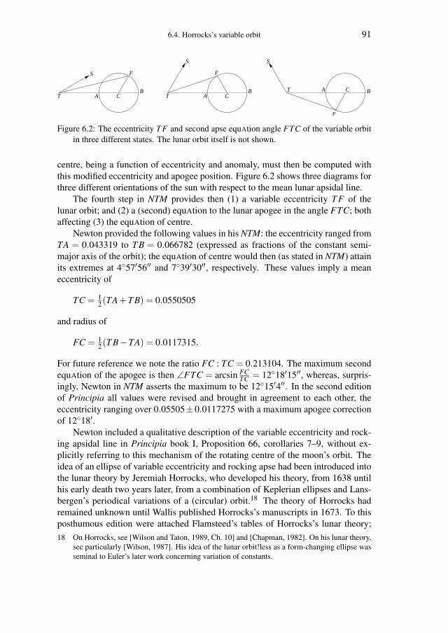
Figure 6.2: The eccentricity T F and second apse equAtion angle FTC of the variable orbitin three different states. The lunar orbit itself is not shown.

centre, being a function of eccentricity and anomaly, must then be computed withthis modified eccentricity and apogee position. Figure 6.2 shows three diagrams forthree different orientations of the sun with respect to the mean lunar apsidal line.

The fourth step in NTM provides then (1) a variable eccentricity T F of thelunar orbit; and (2) a (second) equAtion to the lunar apogee in the angle FTC; bothaffecting (3) the equAtion of centre.

Newton provided the following values in his NTM: the eccentricity ranged fromTA = 0.043319 to T B = 0.066782 (expressed as fractions of the constant semi-major axis of the orbit); the equAtion of centre would then (as stated in NTM) attainits extremes at 4◦57′56′′ and 7◦39′30′′, respectively. These values imply a meaneccentricity of

TC = 12(TA+T B) = 0.0550505

and radius of

FC = 12(T B−TA) = 0.0117315.

For future reference we note the ratio FC : TC = 0.213104. The maximum secondequAtion of the apogee is then ∠FTC = arcsin FC

TC = 12◦18′15′′, whereas, surpris-ingly, Newton in NTM asserts the maximum to be 12◦15′4′′. In the second editionof Principia all values were revised and brought in agreement to each other, theeccentricity ranging over 0.05505±0.0117275 with a maximum apogee correctionof 12◦18′.

Newton included a qualitative description of the variable eccentricity and rock-ing apsidal line in Principia book I, Proposition 66, corollaries 7–9, without ex-plicitly referring to this mechanism of the rotating centre of the moon’s orbit. Theidea of an ellipse of variable eccentricity and rocking apse had been introduced intothe lunar theory by Jeremiah Horrocks, who developed his theory, from 1638 untilhis early death two years later, from a combination of Keplerian ellipses and Lans-bergen’s periodical variations of a (circular) orbit.18 The theory of Horrocks hadremained unknown until Wallis published Horrocks’s manuscripts in 1673. To thisposthumous edition were attached Flamsteed’s tables of Horrocks’s lunar theory;18 On Horrocks, see [Wilson and Taton, 1989, Ch. 10] and [Chapman, 1982]. On his lunar theory,

see particularly [Wilson, 1987]. His idea of the lunar orbit!less as a form-changing ellipse wasseminal to Euler’s later work concerning variation of constants.

92 6. The Horrocks Legacy

and it was Flamsteed who later, in 1694, convinced Newton of the quality of Hor-rocks’s theory. Such happened perhaps at a time when Newton’s own researches onlunar motion were coming to a grinding halt.

Curtis Wilson considered Horrocks’s theory the chief improvement in lunartheory during the 17th and early 18th centuries, thereby implicitly giving it moreweight than Newton’s theory of gravitation and its—currently unclarified—influ-ence on lunar theory: ‘The [Newton’s] approach [to lunar theory] failed, and as apredictive model, Horrocks’s own theory remained as good as any available downto the publication of Tobias Mayer’s first lunar tables in 1753.’19 Wilson’s viewis endorsed by George Smith: ‘Newton himself did not significantly advance theproblem of the moon’s motion beyond Horrocks.’20 On the other hand, Smith doesvenerate Newton’s significant contribution of providing the study of the moon’s mo-tion with a gravitational basis. We must also not forget that more than half of thelongitude equAtions in NTM were original and at least qualitatively, if not quan-titatively, derived from the law of gravitation. We should not, therefore, interpretNewton’s lunar theory as only an improved version of Horrocks’s lunar theory. Onemight say that Newton’s lunar theory was the first to contain equAtions predicted tobe of any relevance, without first having been observed.21

6.5 OLD WINE IN NEW BOTTLES

We will now translate the kinematic Horrocksian model of the previous section intothe language of trigonometric functions. It will become clear that quite a numberof other equAtions are involved. Computations similar to those below were madeby Mayer, which shows his interest in Newton’s NTM. A brief comment on hiscalculations will be made near the end of this section. Later in the chapter, hiscalculations will also be seen to play a crucial role in the conception of the kil

tables.What needs to be done, therefore, is to analyse how the Horrocksian variable

orbit affects the equAtion of centre. For an unperturbed elliptical motion, the equA-tion of centre C may be written to the third order in the eccentricity e as

C =−(2− 1

4e2)esinv+ 54e2 sin2v− 13

12e3 sin3v, (6.1)

where v denotes the mean anomaly measured from the apogee. The key concept ofHorrocks’s variable orbit is to periodically change the eccentricity and the apse lineorientation of the lunar orbit, and to take the equAtion of centre pertaining to theform-changing instantaneous ellipse. Referring to either figure 6.1 or 6.2, we putthe mean eccentricity TC = a, the actual eccentricity T F = e, and the fixed ratioFC : TC = β . The kinematic model specifies that ∠FCB = 2∠STC = 2(ω − p),where p equals the lunar mean anomaly (once equAted for the annual equAtion of19 [Wilson, 1987, p. 77]; also see [Wilson and Taton, 1989, p. 194].20 [Newton et al., 1999, p. 256].21 [Wilson, 1987, p. 77], [Newton et al., 1999, p. 256]; also see [Wilson and Taton, 1989, p. 194].

6.5. Old wine in new bottles 93

the apogee), and ω the mean lunar longitude minus mean solar longitude. Hencewe express the eccentricity via

e2 = T F2 = TC2 +FC2 +2TC FC cos∠FCB

= a2 +a2β

2 +2a2β cos(2ω −2p). (6.2)

For the modified anomaly in (6.1) we write v = p + δ , where, deviating from ourusual meaning of the symbol δ for the duration of this section, δ = ∠FTC, thesecond equAtion of the apogee. Let D (not in figure) be the foot of the perpendicularfrom F to TC. The following relations hold for δ :

sinδ =FDT F

, whence esinδ = aβ sin(2ω −2p),

cosδ =T DT F

, whence ecosδ = a(1+β cos(2ω −2p)

). (6.3)

The equations (6.2) and (6.3), which provide the moon’s variable eccentricity aswell as the second equAtion of the apogee, will be of use again in the next section.Presently, we use them to write the first-order term in the modified equAtion ofcentre as

esin(p+δ ) = ecosδ sin p+ esinδ cos p

= a(1+β cos(2ω −2p)

)sin p+aβ sin(2ω −2p)cos p

= asin p+aβ sin(2ω − p). (6.4)

This is beautiful. The term asin p on the right-hand side is the first-order term ofthe equAtion of centre for the mean eccentricity a and mean anomaly p. The secondterm has argument 2ω− p and we recognize it as the prime evection term. Thus welearn the important fact that the Horrocksian-modified equAtion of centre equals thesum of the unperturbed equAtion of centre and the evection, to the first order in theeccentricity. Next, we combine (6.2), (6.4) and the familiar relation

sinxcosy = 12

(sin(x+ y)+ sin(x− y)

), (6.5)

in order to expand the first term of (6.1) into(2− 1

4e2)esin(p+δ ) =(2a− 1

4a3− 12a3

β2)sin p

+(2aβ − 1

2a3β − 1

4a3β

3)sin(2ω − p)

− 14a3

β2 sin(4ω −3p)+ 1

4a3β sin(2ω −3p).

(6.6)

Continuing now to the second term in (6.1), we first observe that

e2 sin2δ = 2e2 sinδ cosδ

= 2a2β sin(2ω −2p)

(1+β cos(2ω −2p)

)= 2a2

β sin(2ω −2p)+a2β

2 sin(4ω −4p);

e2 cos2δ = e2(cos2δ − sin2

δ )

= a2(1+β cos(2ω −2p))2−a2

β2 sin2(2ω −2p)

= a2 +2a2β cos(2ω −2p)+a2

β2 cos(4ω −4p);

94 6. The Horrocks Legacy

hence

e2 sin(2p+2δ ) = e2 sin2pcos2δ + e2 cos2psin2δ

= sin2p(a2 +2a2

β cos(2ω −2p)+a2β

2 cos(4ω −4p))

+ cos2p(2a2

β sin(2ω −2p)+a2β

2 sin(4ω −4p))

= a2 sin2p+2a2β sin2ω +a2

β2 sin(4ω −2p). (6.7)

We see that the second order term of the equAtion of centre contributes to the vari-ation and also (in the second order) to the evection. Repeating the same procedurefor the third term in (6.1) yields

e3 sin(3p+3δ ) =a3 sin3p+3a3β sin(2ω + p) (6.8)

+3a3β

2 sin(4ω − p)+a3β

3 sin(6ω −3p). (6.9)

Finally then, we find that the equAtion of centre (6.1) expands into

C =(−2a+ 1

4a3 + 12a3

β2)sin p+ 5

4a2 sin2p− 1312a3 sin3p+ 5

2a2β sin2ω

+(−2aβ + 1

2a3β + 1

4a3β

3)sin(2ω − p)

+ 54a2

β2 sin(4ω −2p)− 13

12a3β

3 sin(6ω −3p)

− 14a3

β sin(2ω −3p)+ 14a3

β2 sin(4ω −3p)

− 134 a3

β2 sin(4ω − p)− 13

4 a3β sin(2ω + p).

(6.10)

Upon substitution of the typical Newtonian values a = 0.05505 and β = 0.2131, androunding to arc-seconds, we find that the equAtion of centre in the form-changingellipse equals

C =−6◦18′20′′ sin p+13′1′′ sin2p−37′′ sin3p+5′33′′ sin2ω

−1◦20′36′′ sin(2ω − p)+35′′ sin(4ω −2p)−2′′ sin(2ω −3p)−5′′ sin(4ω − p)−24′′ sin(2ω + p).

(6.11)

Several authors have presented a similar but less extensive analysis.22 In partic-ular Gaythorpe and Wilson showed that the Horrocksian variable orbit is equivalentto the combined equAtion of centre and evection. But Gaythorpe missed the con-tribution to variation of ≈ 5′ sin2ω in (6.10). Because of this contribution, everyHorrocksian lunar theory (i.e., with variable eccentricity and apsidal line pluggedinto the equAtion of centre) necessarily has a variation coefficient of ≈ 35′ insteadof the total ≈ 40′.23

22 These include [d’Alembert, 1756, I pp. 91–93], [Godfray, 1852, p. 60], [Gaythorpe, 1957],[Brown, 1896], and [Wilson and Taton, 1989, p. 198].

23 Gaythorpe’s oversight was corrected by Jørgensen [Jørgensen, 1974]; the point had howeveralready been noted by d’Alembert [d’Alembert, 1756, I p. 93, 253].

6.5. Old wine in new bottles 95

Figure 6.3: Part of an unnumbered folio of Cod. µ]28, showing Mayer’s work on the Hor-

rocksian mechanism. The top half of the folio contains an error, which is corrected inthe bottom half (below the double line). Reproduced with the kind permission of SUB,Göttingen.

Mayer too made computations such as those above, as I discovered on variousloose folio sheets among his work on lunar theory (cf. figure 6.3). The same sheetscarry several other computations that are manifestly connected with his endeav-ours to understand the successive steps of Newton’s lunar theory in the languageof trigonometric quantities. In these computations, Mayer kept terms involvinga3β 2 ≈ 2′′, and rejected a3β 3 ≈ 0.3′′ and a4. Because β 2 ≈ a, he might have re-jected a3β 2 just as well. He treated the trigonometric quantities in a distinctly alge-braical style, as developed by Euler since 1739,24 and very similar to our treatmenton the preceding pages of this section.

24 Euler expounded the calculus of the trigonometric functions in his treatise on the great in-equAlity of Jupiter and Saturn [Euler, 1749a], well known to Mayer. See [Katz, 1987, p. 322],[Golland and Golland, 1993].

96 6. The Horrocks Legacy

The contrast between the geometrical style of Newton and Mayer’s reformula-tion in trigonometric quantities is telling of the change in perception of trigonom-etry which Euler had brought about. This contrast is perhaps even more clearlyperceived when we turn to the lunar tables: first to those of Lemonnier, which arefully based on Newton’s NTM, then to the twist that Mayer gave to Lemonnier’stables.

6.6 LEMONNIER’S VERSION OF NTM

Although Flamsteed did not publish his NTM-based lunar tables, some form ofa copy of his manuscript must have reached France, where Lemonnier adapted itfor publication in his Institutions Astronomiques,25 an enlarged translation of JohnKeill’s Introductiones ad veram physicam et veram astronomiam. Mayer was evi-dently well acquainted with both books.26

Because Institutions Astronomiques was an important source to Mayer, we willnow undertake to appraise the conformity of Lemonnier’s tables with Newton’sprecepts. Our general approach is as follows. Because Lemonnier acknowledgedFlamsteed as his source, we may assume as a working hypothesis that the form ofthe equAtions on which his tables are based, agrees to the Newtonian prescriptionsas discussed above. We then deduce the coefficients in these equAtions from thevalues in Lemonnier’s tables. This is straightforward for some equAtions, but moreelaborate for others. Finally, we check if these equAtions and coefficients indeedreproduce Lemonnier’s tables sufficiently accurate, i.e., to within 1′′ or 2′′.

We now turn to the details, referring to section 6.3 for Newton’s seven steps,and to display 6.1 for the results of the analysis, and, as usual, using the argumentnotation of Mayer.

Newton’s first step comprises three annual equAtions, proportional to the so-lar equAtion of centre. The latter is a formula of the form c1 sinς + c2 sin2ς +25 [Lemonnier and Keill, 1746], also see comments in [Kollerstrom, 2000, pp. 205–14].26 [Forbes, 1971a, p. 83], [Forbes, 1980, p. 120]. Rob van Gent suggested (private communica-

tion) that there might have been an interesting alternative source of information of Flamsteed’stables to Mayer, via Johann Gabriel Doppelmayr (1671–1750). Both Germans were workingtogether in the Homann building during the later 1740’s. Doppelmayr visited England in 1701,where he met Gregory for certain, and Flamsteed and Newton very probably [Gaab, 2001].Newton had then already written his NTM [Kollerstrom, 2000, p. 43]. Gregory had not yetpublished it but at least he might have known it. In 1705, after returning to Nuremberg, Dop-pelmayr published his Latin translation of Streete’s Astronomia Carolina. Although Streete’swork was surely a long-standing classic in astronomy, one might expect Doppelmayr to includethe Flamsteed lunar tables instead of Streete’s—which he did not, suggesting that the newerNewtonian tables made at most no lasting impression on him. Moreover, Flamsteed calculatedhis manuscript lunar tables of the Newton variety only after Doppelmayr had left England, andhe had made apparently only two manuscript copies of them [Baily, 1835, p. 695, 704]. Thetext on the lunar plate of Doppelmayr’s Atlas Coelestis (1742) suggests that the author did notfully grasp the details of NTM. Strikingly, though, Mayer consistently referred to the lunar ta-bles of Flamsteed, never to those of Lemonnier, in his manuscripts. Lemonnier had dutifullyacknowledged Flamsteed as the provenance of his tables.

6.6. Lemonnier’s version of NTM 97

1 Annual equAtionsto longitude +11′49′′ sinς −71

2′′ sin2ς

to apogee −20′ 0′′ sinς +13′′ sin2ς

to node + 9′30′′ sinς − 6′′ sin2ς

2 (+3′45′′−11′′ cosς)sin(2ω −2p)

3 +47′′ sin(2ω −2δ )

4 2nd apogee equAtion arctan β sin(2ω−2p)1+β cos(2ω−2p)

eccentricity e a√

1+β 2 +2β cos(2ω −2p)

equAtion of centre(2e− 1

4e3)sin p−(5

4e2− 1124e4)sin2p

+1312e3 sin3p− 103

96 e4 sin4p

5 Variation (35′15′′−2′11′′ cosς)sin2ω

6 +2′10′′ sin(2ω − p+ ς)

7 −2′20′′ sinω

2nd node equAtion arctan sin(2δ−2ω)γ+cos(2δ−2ω)

Eqn. of Inclination 5◦8′30′′+9′ cos(2δ −2ω)

Display 6.1: EquAtions of lunar longitude, node, and inclination of Lemonnier’s lunar ta-bles. The leftmost numbers correspond to the steps in Newton’s NTM, described insection 6.3.

c3 sin3ς + . . . where ς is the solar mean anomaly, and the coefficients stand in theratio c1 : c2 : c3 = 95 : 1 : 1

69 , roughly. The three annual equAtions should thentake the same form, with the same ratio between the coefficients, while the coef-ficients follow from the extreme values of the equAtions as specified by Newton.This yields the annual equAtions listed in display 6.1; the third coefficients of eachare negligible. Lemonnier’s tables satisfy these equAtions.

Lemonnier’s second equAtion is equivalent to Newton’s second step, and maybe represented as (3′45′′− 11′′ cosς)sin(2ω − 2p). As explained in section 6.3,this equAtion has a seasonal fluctuation in its coefficient. Lemonnier has two tablesto represent this equAtion: one table gives 3′45′′− 11′′ cosς as a function of ς ,the other tabulates 3′45′′ sin(2ω − 2p). The user of these tables has to perform anadditional calculation to establish the magnitude of the second equAtion. If, forgiven values of the arguments ς and 2ω−2p, the first table yields x and the secondtable returns y, then x

3′45′′ y is the value of the second equAtion.A similar seasonal fluctuation is also found in Newton’s step 5, his variation,

which we have represented previously as (35′32′′− 1′53′′ cosς)sin(2ω). Lemon-nier’s fifth equAtion takes two tables again, but his coefficients differ slightly fromNewton’s values: the table for the seasonal part matches 35′15′′− 2′11′′ cosς , theother table lists 35′15′′ sin(2ω).27

27 Lemonnier combined the seasonal tables of equAtions 2 and 5 in one table, for practical reasons.

98 6. The Horrocks Legacy

The third and sixth steps of Newton are easy to implement in tables. For theseequAtions, a straightforward check confirms that Lemonnier apparently adhered toNewton’s coefficients of NTM. He also tabulated Newton’s seventh equAtion exceptthat he dropped its seasonal term.

Finally we come to Newton’s fourth step, with its variable eccentricity and os-cillating apsidal line in the Horrocksian way. Lemonnier implements the motion ofthe apsidal line as a second equAtion of the apogee, but the eccentricity has a moreinvolved rendering. We will illuminate the apogee equAtion first.

In figure 6.1 and equation (6.3), ∠FTC = δ is the second apogee equAtion, andFC : TC = β . It follows from (6.3) that

δ = arctanβ sin(2ω −2p)

1+β cos(2ω −2p). (6.12)

Presuming that Lemonnier tabulated this relation, with ω − p as the argument, weproceed as follows to derive β from his tabulated values: after some manipulationof the formula, we find that

1β

=sin2(ω − p)

tanδ− cos2(ω − p). (6.13)

Now we fill in all pairs of arguments and tabulated values to obtain as many valuesfor β , which when averaged give β = 0.213104. This β substituted back in (6.12)suffices to recreate Lemonnier’s table with no differences larger than 2′′. Besides,this value for β is the same as the ratio for FC : TC = β that we have computed onpage 91 from data in NTM. Thus, Lemonnier’s second apogee equAtion is in perfectagreement with NTM.

To account for the variable eccentricity, Lemonnier again included two tables.The first of these listed the extremal values of the equAtion of centre for differentvalues of the argument ω − p = ∠STC = 1

2∠FCB in figure 6.1. The second ta-ble listed four different equAtions of centre, with, respectively, extremal values of−5◦, −6◦, −7◦, and −7◦39.5′. The user was then supposed to interpolate (or evenextrapolate) between two columns of this table, depending on the extremal valueproduced by the first table. Confusingly, the headings of the second table containednot these extremal values, but the eccentricities at which they occur. The link to theextremes was only explained in a commentary.28

Lemonnier’s table for maximum equAtion of centre can be reproduced to within3′′, as follows: compute the variable eccentricity e according to equation (6.2),with a mean eccentricity of a = 0.05506 instead of Newton’s value 0.05505; thensubstitute this eccentricity in the equAtion of centre, and compute the equAtion forargument p ≈ 94◦.29

28 [Lemonnier and Keill, 1746, p. 629]. The link between argument ω − p and eccentricity e isprovided by equation (6.2) above.

29 The equAtion of centre attains its maximum when cos p = 15e −

√1

(5e)2 + 12 ; for the small ec-

centricities concerned this maximum is reached when p is approximately 94◦.

6.7. ‘Mondtafeln (wahrscheinlich älterer Entwurf)’ 99

With the well-known formula for the equAtion of centre, Lemonnier’s fourfoldtable of that function is then reproducible to 2′′ or better. Interestingly, Lemonnierhad apparently included terms of the fourth order in the eccentricity (see formula inthe middle of display 6.1).

D’Alembert published a similar analysis, but less detailed, missing for exam-ple the second terms in the annual equAtions.30 For completeness, display 6.1 alsoshows Lemonnier’s equAtions for node and inclination; these will not be furtherdiscussed here.31 Kollerstrom rightly remarked that Lemonnier’s tables form atrue representation of NTM, with a few small changes to parameters, without theseasonal modulation of the 7th equAtion, and with the sign error of NTM’s sixthequAtion corrected.32

We have seen that Lemonnier’s tables necessitate multiplications and divisionsto accommodate the seasonally varying equAtions, and that they incorporate a some-what complicated scheme to accommodate the variable eccentricity. A user ofLemonnier’s tables has to make more involved calculations than a user of Mayer’stables, as exemplified in chapter 4.

6.7 ‘MONDTAFELN (WAHRSCHEINLICH ÄLTERER ENTWURF)’

Among the Mayer manuscripts in Göttingen is the quire Cod. µ]15, to which Lichten-

berg added the title ‘Mondtafeln (wahrscheinlich älterer Entwurf)’ (‘Lunar tables,probably of older design’). It is of interest here because it is a witness of the intro-duction of multiple steps in Mayer’s lunar tables. Most of the quire was composedduring 1752. It marked the transition from Mayer’s single-stepped zand theory,contained in a letter to Euler of 1752 January 6, to the multistepped precursors ofthe kil tables published in the spring of 1753.33 Part of its contents depended on adesign considerably older than Lichtenberg might have perceived, as we will see.

The items in the manuscript that are currently of interest, are: (1) a comparisonof the coefficients in several lunar theories on pp. 8v and 9r; (2) tables of lunarequAtions on pp. 9v–16v; (3) a page (p. 17r) with the superscript Entwurf neuer CTafeln; followed by (4) again tables of lunar equAtions. Each of these are discussedbelow, whereafter I provide an interpretation of the manuscript.34

6.7.1 Peering at the peers

The facing folios 8v and 9r of Cod. µ]15 are laid out in the form of an array (see

figure 6.4). The first column on the left side of the array lists trigonometric ex-pressions: successively sin p, sin2p, sin3p, sinς , . . . , sin(p− ς), sin(p + ς), . . . .30 [d’Alembert, 1756, I, Ch. 13].31 The second node equAtion takes γ = 38.3341. These equAtions were demonstrated by Newton

in the Principia. They do not affect lunar longitude.32 [Kollerstrom, 2000, p. 212].33 Letter to Euler: [Forbes, 1971a] p. 48.34 Aliases of the versions treated here are all listed in display A.1 in appendix A.

100 6. The Horrocks Legacy

Figure 6.4: Comparison of coefficients from various astronomers, on fol. 8v and 9r inCod. µ

]15. Reproduced with the kind permission of SUB, Göttingen.

6.7. ‘Mondtafeln (wahrscheinlich älterer Entwurf)’ 101

The other columns bear the following superscripts (numbers added in square brack-ets for ease of reference): [1] Clairaut, [2] Calculus m. ex theor. M., [3] Corr. exobserv. M., [4] Eul., [5] Tabb C. Calc. M., and [6] New. Flamst. Under these head-ings, the columns are filled with numbers, which are clearly coefficients, formingequAtions together with the trigonometric quantities on the left side.

The coefficients in column [3] agree exactly to zand, i.e., to those that Mayertransmitted to Euler in his letter as mentioned above. The letter provides an excel-lent backdrop against which Cod. µ

]15 falls into perspective. In it, Mayer explained

to Euler why he chose to base his tables on the mean arguments, contrary to Euler’spreference for the eccentric arguments:

The angles ω , p, and ς invariably denote the mean motion, which in fact brings several ad-vantages not in the solution, but in practice, because in such a manner the arguments of theinequAlities can be calculated more simply.35

Next in the same letter he referred to the problem of the motion of the lunar apogee.Although the famous problem of its mean motion had recently been solved byClairaut, Mayer’s remark makes more sense when interpreted in relation to the vari-able part of the motion of the apogee, ∠FTC in figure 6.1:

I have indeed always supposed, yet could never be certain, that the inequality associated withthe angle 2ω − p [i.e., evection ], which is without doubt difficult to determine and which wasexplained by Newton as due to the variation of the eccentricity of the Moon’s orbit, stronglyaffects the motion of the apogee. Now, I want particularly to make new attempts to determinethe motion of the apogee, and to see whether I do not arrive at it if instead of the above-mentioned inequality I take the eccentricity as being really variable.36

In fact, this is intelligible only in the context of Newton’s lunar theory and theHorrocksian variable orbit. This remark of Mayer’s presages the multistep tables.In the same letter, Mayer had indicated his desire to see Euler’s and Clairaut’s lunartheories:

Meanwhile, I eagerly await the treatises of yourself and Mr. Clairaut. You would greatly obligeme if I could obtain through your assistance a copy as soon as they are published. . . .37

Euler had been an adjudicator for the 1751 prize contest of the Academy of SaintPetersburg on lunar theory, which was won by Clairaut’s contribution, thereforeEuler was an eminent source of information. He responded on March 18th, 1752that he was unable to compare the magnitudes of the equAtions of his own lunartheory with Mayer’s, because of the differences in the arguments already alludedto: Euler’s tables made use of the eccentric anomaly, but Mayer’s used the meananomaly throughout. Like Mayer’s, Clairaut’s equAtions used the mean arguments,and therefore Euler included a complete list of the equAtions in Clairaut’s theory.Euler kept the equAtions in the same sequence as Mayer had in his letter, insertinga few that were present in Clairaut’s, but absent from Mayer’s theory (most notablyseveral equAtions that involved the angular distance of the sun from the nodes of the35 [Forbes, 1971a, p. 49].36 [Forbes, 1971a, p. 49].37 [Forbes, 1971a, p. 49].

102 6. The Horrocks Legacy

lunar orbit, until then overlooked by Mayer). Mayer copied precisely this list out ofEuler’s letter into column [1] of the array on fol. 8v and 9r of Cod. µ

]15. Therefore

we can be sure that Mayer started this array after he received Euler’s response;moreover, we may speculate that he did not waste much time before doing so.

Mayer’s own coefficients in columns [2] and [3] are mostly identical: appar-ently, he adjusted only a few of the theoretically derived coefficients to observations.The superscript of column [4] suggests that Mayer included coefficients from Eu-ler’s tables. I have not investigated how Mayer obtained these; due to the differencein arguments it was probably a non-trivial exercise.

Column [5] is peculiar in that the coefficients in it sometimes follow Mayer’svalues, sometimes those of Clairaut (particularly for those equAtions where Mayerdid not have a value of his own), and sometimes they fall in between. Only onecoefficient was drawn from Euler’s column, and two are marked as preliminary(‘interim’). It seems as if Mayer was, in a sense, interpolating between his own,Clairaut’s, and (to a lesser extent) Euler’s lunar theories.

Column [6] with its superscript ‘New. Flamst.’ suggests that it is linked toNewton’s lunar theory. Indeed it is: Mayer calculated these coefficients on the samefolios of Cod. µ

]28, mentioned on page 94 above, where he expressed Horrocks’s

variable eccentricity and apsidal line as trigonometric quantities. This column wasadded perhaps a little while after the other columns had been completed.

6.7.2 The first set of lunar tables

The next item of interest in Cod. µ]15 is a set of lunar tables aliased grond. It

contains mean motion tables equivalent to Lemonnier’s, except that the node epochwas adjusted. The mean motions are followed by 19 tables of equAtions cateringfor exactly the equAtions with their coefficients as listed in column [5], fol. 8v. Thesuperscript Tabb C. Calc. M. of column [5], just discussed, refers to these tables.

6.7.3 ‘Entwurf neuer C Tafeln’

Apparently Mayer abandoned those grond lunar tables; they are immediately fol-lowed by a page so revealing that I have transcribed it in display 6.2. The followingobservations apply.

A heading Entwurf neuer C Tafeln is written along the top edge of the page:‘design of new lunar tables’. The design is specified below the heading. Thereare 11 numbered arguments, which are given symbolically as well as in descriptivelanguage. For each argument, an equAtion is specified, with one or more terms,and appropriate coefficients in sexagesimal notation. The majority of the equAtionsapply to lunar longitude, but there are a few that apply to the apogee or node.

The plain-language descriptions of the arguments in the third column clearlyreveal that some of them are to be corrected in steps. The elongation of the moonis to be corrected using the first equAtions, depending on argument ς , the mean

6.7. ‘Mondtafeln (wahrscheinlich älterer Entwurf)’ 103

solar anomaly. Mayer indicates this by his addition ’I corr.’ in the description ofarguments II and V. Similarly, argument IV is the anomaly of a ‘corrected’ moon;Mayer uses the symbol q to distinguish it from the mean anomaly p. There isa similar distinction between the elongations ω and ω̃ , although less consistentlyapplied: argument VI is lunar elongation after application of the Vth equAtion (and,I suppose, equAtions I to IV as well).

To summarize, Mayer introduces the multistep procedure here in this ‘new de-sign’. By the doubled lines between III and IV and between V and VI he clearlydistinguished the three steps.

The basic structure of this design has some striking resemblances to Newton’sNTM, including the following. The first argument, solar mean anomaly ς , is notonly used to equAte the lunar longitude, but also its apogee and node positions.This is a significant influence of Newton on Mayer. At least as significant, we dis-cover the equAtion of centre and the evection close together as equAtions IV andV in the middle step. These are followed by the variation in VI and several sub-sequent smaller equAtions. Among those, numbers VIII and IX take up Newton’sseasonally modified variation; they were most likely derived (at least in form) byapplication of equation (6.5). Differing from NTM, Mayer’s design collects severalequAtions together into one step, and his last two equAtions are new. ApparentlyMayer dropped these two almost immediately afterwards. Also most (but not all)of the coefficients differ from Newton’s.

6.7.4 The second set of lunar tables

On the following pages of the manuscript we find lunar tables in an untidy hand-writing, as if they were a preliminary or intermediate version. However, these ta-bles differ from the new design just discussed. Apart from mean motion tables andan unnumbered equAtion of centre answering to −6◦18′56′′ sin p + 12′55′′ sin2p−32′′ sin3p, we find:

II +40′′ sin(ω − p)+3′20′′ sin(2ω −2p)III −58′′ sin(2ω + ς)IV −58′′ sin(2ω − ς)V −58′′ sin(2ω −2δ )VI +1′30′′ sin(2ω − p+ ς)VII +1′30′′ sin(2ω − p− ς)VIII +58′′ sin(2δ − p)IX +30′′ sin(2δ −2p)X +1′30′′ sin(2ω + p)

At first sight, this does not seem to tally with the multistepped development ofthe Entwurf. However, using techniques described in section 8.4, I analysed cer-tain position calculations in Cod. µ

]41, and discovered that they used the equAtions

embodied in these tables, and moreover that these calculations adhered to a compu-

104 6. The Horrocks Legacy

Ent

wur

fneu

erC

tafe

ln.

Aeq

.CA

eq.a

pog.

Aeq

.F1

Arg

.I.ς

Ano

mal

iam

edia

Solis

+11

′ 40′′ s

inς

−20

′ 0′′

sin

ς&

c−

10′′

sin

2ς+

20′′

sin

2ςA

rg.II

.ω−

pD

istC

aA

Icor

r.+

3′20

′′si

n(2ω

−2p

)−

Ano

mC

med

±20

sin(

ω−

p)2

Arg

.III.

uL

ongA−

Lon

gF

med

.−

1′0′′ s

in2u

Arg

.IV.

q..

.L

ongC

corr

.−A

p.D

corr

.−

6◦18

′ 27′′ s

inq

+12

.38

sin

2q−

37si

n3q

Arg

.V.

2ω−

qad

arg

IIad

d.D

ist.C

aA

I.cor

r.−

1◦21

′ 0′′

sin(

2ω−

p)+

36si

n(4ω

−2p

)A

rg.V

I.ω̃

Dis

t.CaA

post

Vae

quat

ione

m−

2′0′′ s

inω

+40

.21

sin

2ω+

2si

n3ω

+22

sin

4ωA

rg.V

II.

2ω̃−

q+

ςad

arg

Vad

d.an

omA

med

+[?

].10

sin(

2ω−

q+

ς)

Arg

.VII

I.2ω

+ς

adar

gV

IIad

dan

omC

add

arg

IV−

1.10

sin(

2ω+

ς)

Arg

.IX.

2ω−

ςad

dupl

distC

aA

subt

anA

−0.

30si

n(2ω

−ς)

vel1

.0ve

l0.0

Arg

.X.

2ω−

q+

2uad

Arg

Vad

ddu

pl.a

rgII

I.+

1.0

sin(

2ω−

q+

2u)

Arg

.XI

2ω−

2q+

2uab

Arg

Xsu

btr.

Arg

IV+

0.30

sin(

2ω−

2q+

2u)

Dis

play

6.2:

Des

ign

ofne

wlu

nar

tabl

es,t

rans

crip

tion

offo

l.17

rin

Cod

.µ] 15

,alia

sgeer

.T

hesm

alln

umbe

rs1

and

2in

the

left

mar

gin

and

the

dots

afte

rqin

Arg

.IV

are

asin

May

er’s

orig

inal

.The

illeg

ible

coef

ficie

ntin

eqn.

VII

shou

ldre

ad2′

10′′ .

6.8. Accuracy of theories compared 105

tational scheme with multiple steps.38 Unlike what the numbering suggests, theirfirst equAtion depends on ς ; the second step is an equAtion of centre and evection,and the third step is variation. Thus, the computations show a procedure identicalto the zwin version which Mayer wrote to Euler on the 7th of January, 1753, and tothe kil tables which were published in the spring of that year.39

In short, the manuscript Cod. µ]15 contains a list of the coefficients of Clairaut’s

lunar theory, compared to coefficients of Mayer’s own theory at that time (1752), aswell as to their fitted counterparts of gors-zand, and also to coefficients extractedfrom theories of Euler and ultimately (perhaps added a while later) of Newton-Flamsteed-Lemonnier. This is followed first by tables based on a kind of mediatedcoefficients, then by a sketch of the new design that adopted Newton’s multisteppedscheme, and finally by tables of a multistepped nature, which can be regarded aspredecessors of the kil tables.

This may be interpreted as follows. Prior to 1752, Mayer had a lunar theory, andhe had fitted the coefficients to observations. Not being satisfied with the result, hediscussed various aspects of lunar theory with Euler, including a variable eccentric-ity and the uneven motion of the apsides. Euler kindly transmitted the coefficientsof Clairaut. Mayer looked closely at the results of his fellow mathematicians andmingled some of it with his own coefficients, but soon he turned to a Newtonian-like scheme characterized by multiple steps, annual equAtions of node and apogee,and an analytical equivalent of Horrocks’s variable ellipse. This marked the start ofa new branch of development.

6.8 ACCURACY OF THEORIES COMPARED

In order to assess if Mayer reached an improved accuracy by adopting the Newto-nian steps, I conducted the following numerical experiments. I loaded several setsof (Mayer’s and Lemonnier’s) coefficients into a computer program. Each set cor-responded to a different version of tables; and with each set the program computed1000 lunar longitudes at three-day intervals starting Jan. 1, 1740, covering a littleless than half a Saros. These longitudes were subtracted from ones obtained by amodern theory, and the standard deviation of the differences was taken. The re-sults are listed in display 6.3. All the non-modern lunar longitudes were computedusing a modern solar theory40, and all computations were conducted with one and

38 Those calculations on pp. 1–29, 74, 90, 91 apparently used equAtions much like the ones athand, in a context of Mayer developing his tables. His work included improvement of the meanmotions, from those of the first table set mentioned on page 102 above, to those of the publishedkil tables. Mayer compared the outcome of his table computations with observations of JamesBradley that Euler had sent him in the fall or winter of 1752 [Forbes, 1971a].

39 In fact, it appears that the development went from the geer Entwurf via gat and put to zwin,which is almost identical to its successor kil. Improvements of put and kil are discussed inchapter 8.

40 [Meeus, 1998, pp. 163–5].

106 6. The Horrocks Legacy

alias zand grond geer gat zwin kil rede Lemonnierσ [′′] 395 404 96 62 45 43 30 111

Display 6.3: Standard deviations of the longitude terms in some table versions, computedfor n = 1000, starting date 1740 Jan. 1, step size 3 days, Xephem computer programtaken as modern reference. Computations done with the same (zwin) lunar mean mo-tions and with modern solar mean motions. Geer is the Entwurf version.

the same version of Mayer’s lunar mean motion parameters. Therefore the com-putations usually do not reproduce the same lunar longitudes as Mayer would haveobtained himself. This is perfectly reasonable because our goal here is to get animpression of the error distribution of positions generated from various of Mayer’speriodic equAtions. As it turns out, the adopted mean-motion practice has an effectprimarily on the mean of the computed differences, and hardly on their standarddeviations. By using the same solar theory and lunar mean motions with variousequAtion versions, we concentrate on the quality of those equAtions.

Kollerstrom reported that Newton’s lunar theory, with the sign error in the sixthequAtion corrected, had a standard deviation of σ = 1.88′ ≈ 113′′ on 40 samplesat 4-day intervals after 1681.0 using his full computer implementation of NTM. Ifound σ = 123′′ using a somewhat different implementation that had the variableeccentricity and apsidal line represented by trigonometric quantities obtained as insection 6.5. I could discern that small variations to the mean motion parameters hadan impact on the pattern of the position errors, but not on the standard deviationof the errors. Kollerstrom reported σ = 1.9′ = 114′′ for Lemonnier’s tables, whichagrees very well with my determination of 111′′. These correspondences providesome sense of feasibility of my approach. In various other sources, the accuracyof NTM has been quoted as anything ranging from 2′–3′ (by Halley) to 8′–10′ (byFlamsteed) but usually it was not exactly specified to what these numbers referred.41

Clairaut, in his lunar theory, included a list of 100 observations of the mooncompared to positions predicted by his own tables, which also had been slightly ad-justed to observations.42 Interestingly, their standard deviation comes out at 110′′,suggesting that Clairaut’s tables were no better than Lemonnier’s. However, thisconclusion must be treated with considerable care, because the data sets are com-pletely incomparable. A test of the tables that was included in the Connoissancedes Temps for the year 1783, suggests significantly smaller standard deviations.43

Display 6.3 shows that Mayer’s grond version, being presumably an attemptto improve zand by mixing in his peer’s results, did not meet its objective. ButMayer attained a dramatic fourfold increase in performance as soon as he adapted

41 [Baily, 1835, p. 695]. Kollerstrom’s numerical results are taken from [Kollerstrom, 2000,pp. 143–4, 227].

42 [Clairaut, 1752b, p. 91].43 [Lémery, 1780]; part of the difference can be explained by the circumstance that Lémery per-

formed the test with the—fitted—tables of Clairaut’s later (1765) edition of his theory.

6.9. The preface to the kil tables of 1753 107

the Newton/Lemonnier theory. We can imagine that Mayer felt he had discoveredsomething to stick to, even when he lacked our modern statistical concepts.

When his kil tables went to the press less than a year later, he had again dou-bled the accuracy. In the decade between the 1752 zand variant and the final redetables, Mayer gained a factor 13 in the accuracy of his equAtions, measured by theirstandard deviations. His changes in mean motion parameters are not taken intoaccount here.

6.9 THE PREFACE TO THE KIL TABLES OF 1753

Because I have conjectured that the kil tables published in the Göttingen Commen-tarii44 developed out of Mayer’s embracing of NTM, it will be interesting to holdMayer’s own comments to those tables up against that conjecture, in particular withregard to their kinematic vs. dynamical background.

In his introduction to those tables, Mayer asserted that he had deduced the in-equAlities out of ‘that most famous theory of the great Newton’, which Euler hadfirst reduced to ‘analytical equations’, and which Mayer had himself—after severalfruitless attempts—solved ‘by a singular and sufficiently elegant method’, althoughit would be too lengthy for him to explain how. Instead, he elaborated on the causeof the equAtions.45

From the vantage point of our current conjecture we begin to wonder whichof Newton’s ‘theories’ he addressed: the theory of gravitation, or NTM? At firstsight, his reference to Euler is with regard to the casting of Newtonian physics in thelanguage of differential equations. But couldn’t Mayer have had Euler’s codificationof trigonometric functions in mind, as a prerequisite to translate NTM into thatformalism? Could his ‘singular and elegant method’ refer to the translation of theHorrocksian mechanism into the language of trigonometric functions? If so, thatcould explain why Mayer was silent about his method, for Newton’s NTM mighthave been regarded as old-fashioned compared to the analytical advancement of44 The tables were published, with an introduction, as [Mayer, 1753b]. In the Gentleman’s Maga-

zine for August 1754 appeared an almost littoral translation into English of their preface, whichForbes in turn included in [Forbes, 1980, pp. 143–146].

45 ‘Yet I have deduced these tables, so far as the inequAlities of motion are concerned, from thatmost famous theory of the great Newton; which the celebrated Mr. Euler has firstly reducedmost elegantly to general analytical equations. In solving these equations, after trying otherways in vain, I have used a particular and quite elegant method, but to exhibit it here wouldtake too long. Therefore I have resolved to disclose only those things that make it possible tosee through the origin and causes of the inequAlities presented in the tables, so far as one canwithout calculation’ (‘Deduxi autem has tabulas, quoad inaequalitates motuum, ex famosis-sima illa magni Newtoni theoria; quam Vir Celeberrimus EULERUS primus ad aequationesanalyticas generales elegantissime reduxit. Usus sum in hisce aequationibus resolvendis postfrustra tentatas alias vias methodo singulari satisque concinna, sed quam hic exponere nimislongum foret. Quapropter ea tantum indicare decrevi, quae ad originem causasque inaequali-tatum in tabulis exhibitarum, quantum quidem sine calculo licet, perspiciendas facere possunt’)[Mayer, 1753b]. D’Alembert criticized that it was not Euler, but he himself and Clairaut, whohad first produced analytical lunar theories [d’Alembert, 1756, I p. 252].

108 6. The Horrocks Legacy

Euler and Clairaut. But Mayer’s remark of finally attaining a solution after fruitlessattempts seems to refer rather to gravitation and differential equations again. Hismessage to the reader is of having deduced the tables from the Newtonian theory ofgravitation. Yet, the NTM-like structure of the tables and the inadequate state of histheory at that time suggest otherwise.

Instead of supplying the reader with an account or even a sketch of his theory,Mayer chose rather to construe the nature of the various equAtions. After he hadexpounded both the equAtion of centre and the evection, he related these two equA-tions to the variable eccentricity and apse movement as explained by Newton:

By those XIth and XIIth equAtions [i.e., the equAtion of centre and evection ], the same inequA-lities are saved that Newton and those who have closely followed him have explained by avariable eccentricity of the lunar orbit and an unequal motion of the apsides. And althoughthat method [of Newton] answers exactly to the theory, as indeed I can demonstrate, yet it issomewhat more difficult and almost useless for table calculation. The astronomy of the moonowes therefore much to the celebrated Euler. He has been the first who elegantly put a constantequAtion of centre linked with what we have called the evection, in the place of a variableeccentricity, and in this way he has furnished the theory of the moon, otherwise extremelyintricate, with distinguished profit.46

Thus, Mayer showed in this text that he was well acquainted with NTM. He saidthat its variable orbit was not suitable for lunar tables, and he praised Euler forsubstituting a fixed orbit with a constant equAtion of centre—not a word aboutdifferential equations or forces! Strictly, the passage does not imply that there wasno coherent theory supporting Mayer’s tables. One wonders, though, in what wayhe saw Newton’s variable eccentricity and apse as justified exactly by theory.

Continuing his tale, Mayer recognized that the variable distances between earthand sun, and also between moon and earth, give rise to periodic alterations of theevection and variation. For the evection, these alterations are expressed by equA-tions depending on arguments 2ω ± ς , 2ω − 2p, and a part of the variation (argu-ment 2ω). For the variation, they bring about equAtions depending on 2ω ± ς and2ω ± p; the 2ω − p effect being part of the evection. We have seen that some ofthese equAtions are implicitly present in NTM, in the form of coefficients varyingannually with the mean anomaly of the sun. Mayer had no trouble to translate theseinto the form of his own tables.

In conclusion, Mayer offered very little in this preface to support his allegeddynamical theory. He carefully avoided to assert that he indeed had such a theory:his comments about it are evasive. On the other hand, the kinematics of NTM clearlyshow through.

46 ‘Duabus istis aequationibus XI nempe & XII eaedem inaequalitates salvantur, quas Newtonus,& qui stricte eum secuti sunt, per variabilem eccentricitatem orbitae lunae & inaequalem ap-sidum motum explicuerunt. Et quamquam ista methodus theoriae, quod equidem demontrarepossum, exacte respondet, paulo tamen est difficilior & ad calculum tabularem fere inepta. Mul-tum igitur debet astronomia lunaris Cel[ebri] EVLERO. Is enim primus fuit, qui constantemaequationem centri iunctam cum ea quam evectionem diximus, loco eccentricitatis variabilisconcinne substituit, eoque theoriam lunae alias maxime intricatam insigni compendio ornavit’[Mayer, 1753b, p. 385]; also see [Forbes, 1980, p. 143].

6.10. Conclusion 109

6.10 CONCLUSION

I have shown that Mayer had a strong interest in NTM at a time when his own lunartheory was still very imperfect and incomplete. He compared his own results (i.e.,gors) with those of others: first with Clairaut and Euler, leading to the soon-to-be-abandoned griend/grond variety of tables; and then with Newton’s ‘theory’, whichinspired him to the geer version modelled after Newton’s theory. Several folios inCod. µ

]28 attest Mayer’s engagement with Newton’s lunar theory and his ability to

translate its equAtions into the analytical language of trigonometric quantities. Al-though the dating of those folios is uncertain, their results are largely in accord withthe list in Cod. µ

]15, fol. 9r, in the column under the heading New. Flamst. There

Mayer started a line of development characterized by the multistep scheme of appli-cation, with the middle step equivalent to the Horrocksian kinematics. ManuscriptCod. µ

]15 in combination with the Mayer-Euler correspondence show how Mayer

embraced the essence of the computational scheme of Newton’s lunar theory dur-ing 1752. Mayer’s remarks to Euler in a letter of January 1752, quoted above onpage 101, presage this development.

Mayer’s change of strategy seems to be made for pragmatic rather than theo-retical reasons. It happened when his results remained inadequate, when he waslooking around for inspiration, and when he had shared with Euler his intentions toemploy a variable eccentricity as in Newton’s theory. The standard deviations listedin display 6.3 show that the new plan, embodied in the Entwurf neuer C Tafeln,brought about a dramatic fourfold increase in accuracy. The reason for the surpris-ing increase in accuracy after adoption of Newton’s scheme should be the subjectof further research.

I am not aware of any position computations that immediately showed to Mayerthe success of his new scheme, neither have I seen indications that his changewas theoretically motivated. In the next chapter I will show that all the multi-stepped computational schemes can be transformed into a single-stepped scheme;this implies that—as far as accuracy is concerned—there is no real advantage ofany scheme over any other. In other words, the multistepped scheme is not reallynecessary, and eventually we have to address the question why Mayer adhered to itonce he had the technical tools to get rid of it.

Mayer introduced the multistepped procedure in this stage of his work as aconsequence of the assimilation of Lemonnier’s lunar tables, which were rooted inFlamsteed’s rendering of NTM, while NTM in turn incorporated Horrocks’s variableellipse. Lemonnier’s tables necessitated the user to perform quite involved addi-tional computations, associated with the variable eccentricity and the seasonal fluc-tuations of some equAtions. In contrast, Mayer’s tables were much more straight-forward to apply. In his preface to the kil tables, Mayer credited Euler for pro-viding the means to make the transition. We must understand his allusions to Eulernot in connection with a dynamical lunar theory, but rather in connection with thechanging perception of trigonometry which the latter had brought about. It is hard

110 6. The Horrocks Legacy

to imagine that the computations in section 6.5 would have been performed if ev-ery sine and cosine were regarded as half a chord in a circle. Among the advancesin celestial mechanics taking place in the 18th century, the changing perception oftrigonometry may well have been as important a development as the advent of thedifferential calculus.

The new Entwurf soon developed into the kil tables, printed in 1753. Mayerwas so proud of the latter that he boasted to Euler:

So much is certain, that the tables give the Moon’s position as accurately as could hitherto havebeen obtained through observations, and that therefore no greater reliability in these can besupplied or hoped for until more diligence is first of all applied to the method of observing.47

The accuracy of kil was widely recognized and highly appreciated; the tables wereeven accurate enough to bring the application of the lunar distance method of lon-gitude determination within reach. Thus, Mayer was encouraged to enter the questfor the Longitude Prize. Therefore these tables play a key role in Mayer’s workon lunar motion. In their introductory comments Mayer showed that he had a firmunderstanding of the physical meaning of each of its equAtions. Yet, contrastingwith Mayer’s claim, in the light of their NTM-like way of application it is unlikelythat the kil tables of 1753 were backed by a coherent lunar theory on a dynamicalbasis. There may have been partial results derived from such a theory, e.g., his newequAtions of arguments p− ς and 2ω − p− ς . Such results may perhaps providethe reason why Mayer was able to quickly improve upon Lemonnier’s tables.

At least one contemporary astronomer might possibly have recognized the linkbetween Mayer’s kil tables and the Newton/Lemonnier theory, had he been search-ing for it. This was d’Alembert, who went to great lengths to compare his own lunartheory to Lemonnier’s tables. He even preferred to present his own results in the for-mat of those tables. Kil reached d’Alembert while the last pages of his own theorywere being printed, and he had just enough time left to wedge in a contemptuouscomment on them. He did make an effort to compare several theories includingMayer’s, even recognizing that Mayer’s tables came closest to his favourite tablesof Lemonnier; but apparently he did not recognize that they relied on the same kine-matic model. Instead, he wondered whether Mayer had adopted Euler’s theory, orwhether he had a theory of his own.48

Petrus Frisius compared the theories of Newton, Clairaut, Euler, d’Alembertand Mayer. He was able to convert the Horrocksian kinematic mechanism of New-ton’s NTM into trigonometric expressions and he also recognized that the positionof evection had changed between Mayer’s kil and rede tables. Yet he too was

47 Mayer to Euler, May 7, 1753, [Forbes, 1971a, pp. 65–66].48 [d’Alembert, 1756, I pp. xxvi, 250–252]. The quantitative statements of d’Alembert do not all

seem to make sense; e.g., he asserted that Mayer’s evection is effectively very different fromLemonnier’s, while in truth both are almost the same after conversion into comparable form.Later, d’Alembert recognized that Mayer’s kil tables were the most accurate available and alsothe most practical to use, whereupon he constructed new lunar tables with a multistep format[d’Alembert, 1780, II, p. 271–312].

6.10. Conclusion 111

unable to discover the link between NTM and kil.49 The form in which NTM waspresented, be it in Newton’s descriptive pamphlet or in Lemonnier’s tables, wasapparently just too different from Mayer’s kil tables.

The final implication of all this seems to be that the influence of the differentialcalculus on the success of Mayer’s lunar tables of 1753 is much less significant,and the impact of Newton’s 1702 theory (more specifically, its implementation byFlamsteed as published by Lemonnier) much more significant, than has hithertobeen assumed. The success of Mayer’s 1753 lunar tables depends on a hybrid mixof these two ingredients, with a firm dash of coefficient fitting as a third component.

49 [Frisius, 1768, pp. 272–3, 357].