694 IEEE TRANSACTIONS ON ROBOTICS, VOL. 22, NO....

694 IEEE TRANSACTIONS ON ROBOTICS, VOL. 22, NO. 4, AUGUST 2006

The Power Dissipation Method and KinematicReducibility of Multiple-Model Robotic Systems

Todd D. Murphey, Member, IEEE, and Joel W. Burdick, Member, IEEE

Abstract—This paper develops a formal connection between thepower dissipation method (PDM) and Lagrangian mechanics, withspecific application to robotic systems. Such a connection is neces-sary for understanding how some of the successes in motion plan-ning and stabilization for smooth kinematic robotic systems canbe extended to systems with frictional interactions and overcon-strained systems. We establish this connection using the idea of amultiple-model system, and then show that multiple-model systemsarise naturally in a number of instances, including those arising incases traditionally addressed using the PDM. We then give neces-sary and sufficient conditions for a dynamic multiple-model systemto be reducible to a kinematic multiple-model system. We use thisresult to show that solutions to the PDM are actually kinematicreductions of solutions to the Euler–Lagrange equations. We areparticularly motivated by mechanical systems undergoing multipleintermittent frictional contacts, such as distributed manipulators,overconstrained wheeled vehicles, and objects that are manipu-lated by grasping or pushing. Examples illustrate how these re-sults can provide insight into the analysis and control of physicalsystems.

Index Terms—Contact modeling, dynamics, frictional contacts,kinematic analysis, modeling for control.

I. INTRODUCTION

MANY mechanical systems, though intrinsically second-order in their governing dynamics, can be adequately de-

scribed by first-order equations of motion, that is, one can oftenpropose a “quasi-static” or “kinematic” version of the governingequations of motion for the purposes of system analysis or con-trol design. The benefits of this simplification are numerous: thedimension of the state space drops by half; the control inputs gofrom being force inputs to being velocity inputs (which are oftenmore easily realized in practice); and the governing equationstypically take a simpler form than the full dynamic model. Ad-ditionally, kinematic systems, although potentially nonlinear, donot typically involve drift terms. There is a greater quality andquantity of nonlinear control results available for driftless sys-tems, as compared with systems with drift. See [1]–[6] for justa few examples.

Manuscript received November 7, 2004; revised July 22, 2005. This paperwas recommended for publication by Associate Editor D. Prattichizzo andEditor H. Arai upon evaluation of the reviewers’ comments. This work wassupported in part by the National Science Foundation under Grant NSF9402726through its Engineering Research Center (ERC) program. This paper was pre-sented in part at the International Conference on Robotics and Automation,Seoul, South Korea, 2001, and in part at the Conference on Decision andControl, Maui, HI, 2003.

T. D. Murphey is with the Department of Electrical and ComputerEngineering, University of Colorado, Boulder, CO 80309 USA (e-mail:[email protected]).

J. W. Burdick is with the Department of Engineering and Applied Science,California Institute of Technology, Pasadena, CA 91125 USA.

Digital Object Identifier 10.1109/TRO.2006.878971

This paper has several interrelated goals. One of the maintechnical goals of this paper is to determine the formal condi-tions under which such reductions can be achieved for multiple-model systems. In multiple-model systems (see Section IV), thesystem’s governing equations switch between several possiblemodels that describe the system’s evolution. This paper presentsnecessary and sufficient conditions for a multiple-model systemto be kinematically reducible; i.e., the second-order dynamicalmodels can be reduced to first-order kinematic models of theform in Definition 4.1. The necessary and sufficient conditionsfor kinematic reducibility of smooth dynamical systems werefirst developed by Lewis [7]. One of this paper’s contributionsis the extension of kinematic reducibility theory to the mul-tiple-model case.

While our kinematic reducibility results can be applied toa large class of problems, we are particularly motivated bythe multiple-model systems that arise frequently in roboticspractice. The multiple-model framework has recently receivedan increasing amount of attention in the control community[8]–[11], so there are many control results available for our use.Therefore, understanding the connection between problems inrobotics and the multiple-model framework will be productive.Examples of multiple-model systems include robotic systemsinvolving intermittent mechanical contacts, such as distributedmanipulators, overconstrained wheeled vehicles, and objectsthat are manipulated by grasping or pushing (see Section X).A number of similar approaches have been proposed or usedto create “quasi-static” models of such systems. Most repre-sentative of these is the power dissipation method (PDM) (seeSection V) introduced by Alexander and Maddocks [1] in thecontext of overconstrained wheeled vehicles. Peshkin also usedsimilar ideas in the study of pushed objects [12]. Based on thismethod, one can develop first-order (or kinematic) equationsof motion for mechanical systems that undergo intermittentsliding contacts. We show in Section VII that solutions to thePDM are multiple-model systems. We have used the PDM tomodel distributed manipulation systems that generate motionvia frictional contacts [13]. The resulting multiple-modeldescriptions are very amenable to control analysis, and theassociated nonsmooth control laws worked well in practice.

As a second goal of this paper, we address a key question:does the PDM produce models that are consistent with a com-plete dynamic (Lagrangian) analysis? The formalization of thePDM and the analysis of its relationship to Lagrangian anal-ysis are the other main contributions of this paper. Formally,in Section IX, we show that every solution to the PDM is pre-cisely a reduction of a solution to the Lagrangian formulation.Moreover, this is true for all solutions, which is important, as

1552-3098/$20.00 © 2006 IEEE

MURPHEY AND BURDICK: PDM AND KINEMATIC REDUCIBILITY OF MULTIPLE-MODEL ROBOTIC SYSTEMS 695

solutions are not unique in either the PDM or the Lagrangianformulation (when nonsmooth interactions, such as impacts andfriction, are taken into consideration).

The paper is organized as follows. To motivate our results,we first examine some examples of mechanisms that naturallyinvolve stick/slip phenomena in Section II. Then, we brieflyreview the classical Lagrangian approach in Section III beforecovering the basic ideas of the multiple-model formalismin Section IV. We then specifically address an example inSection VI using these ideas. In Section VII, we cover charac-teristics of the PDM, and we then move on to reduction theoryfor multiple-model systems in Section VIII. Section IX relatessolutions to the PDM to solutions to the Lagrangian analysis.We end in Section X with a detailed look at several examplesin which we have found our analysis to be practically useful.

II. EXAMPLES

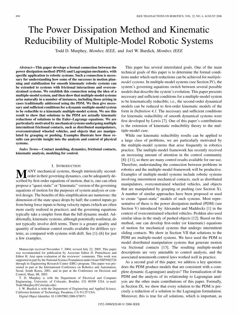
To show the potential breadth of applications for our results,here we summarize four typical robotic and physical systemsto which our theory applies (see Fig. 1): a wheeled bicycle, theRocky 7 prototype of the NASA Mars rover family, a distributedmanipulation system whose function is to manipulate a planarobject via roll-slide contacts, and a multifingered robotic hand.All of these systems are characterized by complex mechanicalinteractions involving contact mechanics and slip. More specif-ically, all of these systems can be modeled and analyzed usingthe multiple-model framework developed in this paper.

Consider the bicycle in Fig. 1(a). For simplicity, we assumethat the bicycle is constrained to move along a line and that bothwheels are actuated. (We will repeatedly return to this example,as it exhibits many of the features that are relevant to our discus-sions). If both wheels are actuated using nonbackdrivable mo-tors, driving both wheels at exactly the same velocity is a diffi-cult task, and thus, this bicycle would typically experience smallamounts of slipping in practice. More interestingly, this slippingis likely to change over time due to variability in contact fric-tion characteristics, leading to a multiple-model, or hybrid, me-chanical system. The multiple-model methodology introducedin this paper and companion papers is well suited to analyzesuch systems.

The NASA Mars rover family members have six indepen-dently driven wheels, as well as two wheels independentlysteered. As discussed in [14] and [15] and reviewed inSection X, this vehicle’s suspension is kinematically overcon-strained, implying some of these wheels are always slipping.Moreover, it can be difficult to predict which wheels slip atany given moment. There is already extensive literature onwheeled vehicles, establishing controllability based on a Liealgebra rank condition (LARC) [16], [17], stability based oncenter manifold theory [6] and hybrid systems theory [11],motion planning based on Voronoi diagrams [18], and RRTs[2]. However, all of these methods assume that the vehiclemotions are governed by smooth, kinematic equations of mo-tion. Because of the inherent and unpredictable switches inslipping, the governing dynamics are not smooth. Nevertheless,the methods developed in this paper show that such vehiclesare still kinematic systems, albeit nonsmooth ones. Moreover,

Fig. 1. (a) Bicycle with both wheels driven. (b) Mars rover Rocky 7 Sojournerprototype. (c) Distributed manipulation testbed developed at Caltech (see de-scription in the text). (d) Hand capable of grasping objects.

in related work, we have made progress on extending classicalnonlinear control concepts, such as the LARC, to the domain


of multiple-model systems [14]. We will discuss this more inSection X-B.

Distributed manipulation has received recent attention in therobotics community [19], [20]. Fig. 1(c) shows a distributed ma-nipulation testbed developed by the authors, in which nine ac-tuated wheels can be used to manipulate planar objects set uponthe manipulation surface. All of these wheels can be indepen-dently driven and steered, giving the system 18 control inputs,with only the position and orientation of the manipulated ob-ject as the output. Hence, this system is massively overactuated.The idea of many actuated devices interacting with an object toachieve some desired manipulation goal is appealing, partiallybecause of its scalability and the possibility of using many inex-pensive actuators rather than a few expensive ones. Moreover,microelectromechanical system (MEMS) fabrication technolo-gies potentially enable distributed manipulation to be a leadingcandidate for micromanipulation. We have shown in prior workhow distributed manipulators that employ frictional contacts fallinto the multiple-model domain [13]. The multiple-model kine-matic reducibility theory developed in this paper provides asimple but rigorous framework for the design of stabilizing con-trol laws that take into account the nonsmooth effects of friction.We have used kinematic reductions both to show the potentialshortcomings of control laws based on smooth idealizations, andto explicitly compute stabilizing control laws that work well ex-perimentally (see [13]).

Grasping and locomotion continue to be active areas ofrobotics research. Current methods often use kinematic models[3] to represent the system dynamics, yet grasping implicitlycontains many of the previously mentioned difficulties. Inparticular, although stick/slip phenomena occur in a graspingproblem, there are not very convincing ways to show thatthe kinematic methods typically used for grasping are robustwith respect to the variation in stick and slip states for a givencontact. The analytical methods presented here create a methodfor analyzing these difficulties without resorting to dynamic,second-order analysis.

In Section X, we will revisit these examples in order to showhow the kinematic reduction theory of this paper can providesimplification or insight.

III. BACKGROUND: LAGRANGIAN MODELS

WITH FRICTIONAL CONTACTS

This study has been largely motivated by the problem ofmodeling and controlling mechanical systems that experiencemultiple, possibly intermittent, contacts that involve friction,particularly Coulomb friction. Clearly, the contacts placeconstraints on the system’s evolving motions. Constrainedmechanical systems can be modeled using conventionalLagrangian mechanics through the use of Lagrange multipliers.Consider a generic mechanical system with up to frictionalcontacts between rigid body surfaces, where the contacts canbe intermittently slide or stick. Such a system admits up topossible contact states which represent all possible permuta-tions of sliding and sticking. Let denote the system’sLagrangian (kinetic minus potential energy), wheredenotes the configuration of the mechanical system, and is

the -dimensional configuration manifold. If the th physicalcontact does not slip, the contact imposes a nonholonomicconstraint on the mechanical system’s motion. This constraintcan be expressed in the form . If the th contact slips,the Coulomb friction law (which is reasonably accurate forlow-speed/low-acceleration maneuvering) states that the tan-gential reaction force at that contact is ,where , , and are, respectively, the Coulomb frictioncoefficient, normal force to the contacting surface, and slippingvelocity of the contact at the th contact. Hence, the mechanicalsystem’s overall equations of motion can described by

(1)

where is the slipping contact set, the are undeterminedLagrange multipliers, and are the generalized applied forces,that is, if the th contact is slipping. If the th contact isnot slipping, corresponds to the tangential reaction force thatis needed to maintain the no-slip constraint at the th contact.We generally assume in this paper that the contact normal forces

are known. If this is not the case, then solving for the re-action forces can be difficult, involving algebraic relationships[17]. However, additional Lagrange multipliers may often beadded to solve for these normal forces. Note that this descriptioninvolves a choice of coordinates. The equivalent, coordinate-in-dependent representation is the formalism in which we addressthese problems, and is briefly reviewed in the Appendix.

There are two primary practical problems with theLagrangian modeling approach. First, one must solve forthe Lagrange multipliers, a tedious task that often leads tocomplex equations. Second, an additional (and often sensitive)analysis is necessary to determine which contacts are slip-ping at any given instant. Consequently, the practical need toanalyze such systems in a tractable way motivates the use ofquasi-static or kinematic approximations, and, in particular,the PDM that is reviewed in Section V. A natural questionarises when using quasi-static analysis: what is the relationshipbetween the equations of motion predicted by quasi-static anal-ysis and those generated by Lagrangian analysis? Moreover,can the quasi-static equations properly predict the motions ofthe true system? Section IV briefly reviews the concept of amultiple-model system, which is the appropriate mathematicalsetting for this question in the case of intermittent frictionalcontacts. We describe a method for finding quasi-static equa-tions of motion in Section V, and we answer these questions inSection IX.

IV. BACKGROUND: MULTIPLE-MODEL SYSTEMS

We use the formalism of multiple-model systems to addresskinematic reducibility of systems involving frictional and inter-mittent contact.

Definition 4.1: A control system evolving on a smooth-dimensional manifold with inputs is said to be a mul-

tiple-model driftless affine (MMDA) system if it can be ex-pressed in the form

(2)


where . For any and , the vector field assumes a valuein a finite set of vector fields: , where isan index set. The vector fields are assumed to be analytic in

for all , and the controls are piecewise constantand bounded for all . Moreover, letting denote the “switchingsignals” associated with

the is measurable in .Definition 4.1 implies that the control vector fields may

change, or switch, among a finite collection of vector fields,each representing a single smooth model in a set of models .An example of such a system is a vehicle whose wheels canpotentially skid. The system’s governing dynamics will varywhen the wheels slip or do not slip. Such systems are intimatelyrelated to multiple-model systems, such as those studied in[11]. However, we should emphasize that the “switching” isnot like the switching phenomena found in [21]–[24], or astypically studied in the hybrid control systems literature (e.g.,[25] and [26]). In these studies, the switching phenomena ispart of a control strategy to be implemented in the controller.In our case, the switching is induced by environmental factors,such as variations in the contact state between rigid bodies.Since the phenomena which govern the switching behaviormay not be precisely characterized, we make no assumptionsabout the nature of the switching functions, except that theyare measurable (i.e., is a Lesbesgue measurable function inDefinition 4.1). A long-term goal of our work is to developsystematic methods for analyzing control systems with thetype of hybrid (and therefore, nonsmooth) structure seen inDefinition 4.1.

To distinguish between the overall control system andthe smooth control systems that comprise it, we define theindividual control systems to be the smooth control sys-tems making up the multiple-model system, comprisedoffor for some . A system will betermed a multiple-model affine system if it has the form

,where the vector field (or “drift term”) is also selectedfrom a set of analytic vector fields .

V. OVERVIEW OF THE PDM

The idea that many systems minimize power or energy dis-sipation during their state evolution is an old one, but, to thebest of the authors’ knowledge, was first applied in a roboticscontext in [1]. This idea, called the PDM, is a powerful one be-cause it gives an alternate method for deriving equations of mo-tion. In fact, the equations of motion it predicts are first-order,as we shall see. Moreover, the resulting equation of motion havesome unintuitive properties; they are discontinuous and some-times set-valued, and do not typically have unique solutions.Despite these technicalities, the equations of motion are veryuseful for resolving overconstrained systems’ equations of mo-tion. This section describes the principle in the form relevant to

multiple point contact. Section VI goes through a detailed ex-ample as an illustration, and as a way of comparing the PDMto the more traditional Lagrangian mechanics. Section VII thendiscusses some basic properties of the PDM, primarily focusingon uniqueness of solutions. Then, after developing some rele-vant mathematical machinery in Section VIII, we show that so-lutions to the PDM can be directly related to solutions of theLagrangian formulation of the equations of motion.

Now we consider the mathematical statement of the PDM.Let again denote a system configuration. This configura-tion will potentially consist of both group variables (that cor-respond to the unknowns in the state evolution) and shape vari-ables (that correspond to the control inputs in the system).In this case, the configuration manifold can be written as theproduct of and (i.e., ). The relative mo-tions between moving objects at a point contact can be writtenin the form . If , then the contact point is notslipping, while if , then describes the contactpoint’s slipping velocity. The power dissipation function mea-sures the object’s total frictional energy dissipation due to con-tact slippage.

Definition 5.1: Consider a mechanical system (which con-sists of a single rigid body or a set of rigid bodies) that main-tains frictional contacts, where some or all of the contacts maybe slipping. The dissipation or friction functional for -contactstates that are governed by Coulomb friction is defined to be

(3)

where describes the relative slipping velocity, is theCoulomb friction coefficient, and is the normal force at theth contact.

The form of this function reflects the Coulomb friction model,but it can easily be extended to different friction models (see[27]) by replacing the linear term with a more generalstate-dependent function . Now, it is clear from the formof that if , then , that is, whenevera contact slip’s energy is dissipated. Based on this observation,Alexander and Maddocks [1] proposed the following axiomaticstatement of the PDM for an contact system.

Power Dissipation Principle: Given a system withconfiguration and fixed,a system’s motion at any given instant is the one thatminimizes [see (3)] with respect to , that is, find

such that

The PDM is built upon this axiom. It allows one to computeequations of motion purely based on the dissipation functional

. Note that because the minimization occurs over, the solution to the minimization problem is an element

of . Therefore, the equations one gets using this method arenecessarily first-order equtaions. Hence, we may get rid of someof the complexities associated with the Lagrangian mechanics.However, simple is not always correct, so we must understand


the relationship between the Euler–Lagrange equations, whichare known to be equivalent to Newton’s laws, and solutions tothe PDM. In Section IX, we draw this connection by showingthat solutions to the PDM are in one-to-one correspondence to aspecial subset of the solutions to the Euler–Lagrange equations.The fact that solutions to the PDM cannot represent all pos-sible solutions to the Lagrangian formulation can be easily seenby considering the following example. Consider a particle con-strained to move on a surface, with friction between the particleand the surface. There are no controls, so . Lagrangiananalysis suggests that there are two possible contact states, oneslipping and one not slipping. Because and

is the unique minimizer for , the PDM

predicts that the particle will not slip. Hence, it misses some ofthe contact states predicted by the Lagrangian framework. How-ever, the nonslip motion that it does predict is consistent with aLagrangian analysis.

For overconstrained systems with control inputs, the PDMleads to more interesting and useful results. When a configura-tion can be decomposed into two components

, then andthe PDM minimization becomes , that is, the

PDM will predict given . In most cases of interest, the vari-able corresponds to the control inputs, while the variablecorresponds to the system motion of interest. In Section VI, weconsider this case using the simple example of a two-wheel-drive bicycle constrained to move on a line.

VI. EXAMPLE: A TWO-WHEELED BICYCLE

Here, we consider in detail an example to illustrate the sim-ilarities and differences between the Lagrangian and PDM for-mulations of the equations of motion. Consider the planar bi-cycle [see Fig. 1(a)] which is constrained to move along a line.We will revisit this example shortly using the PDM formalism,but for now, we treat it in the Lagrangian framework. Let

, where is the front wheel angle, is the rearwheel angle, and denotes the bicycle’s relative translationof its body frame along the -axis of the world frame .The downward normal force on each wheel depends uponthe bicycle’s weight distribution and, at each point of contact,the coefficient of friction is . Assume that each wheel is ac-tuated, with torques and , and that each wheel may pos-sibly slip. Each wheel has the same moment of inertia

, where is the radius of the wheel andis the mass of the wheel. Finally, the bicycle’s total mass is .Hence, the Lagrangian for this system is

. There are two nonholonomic constraints associ-ated with this sytem, one for the nonslip constraint associatedwith the front wheel and one for the back wheel. These non-slip constraints can be written as and

.Using (1) and solving for the Lagrange multipliers, there are

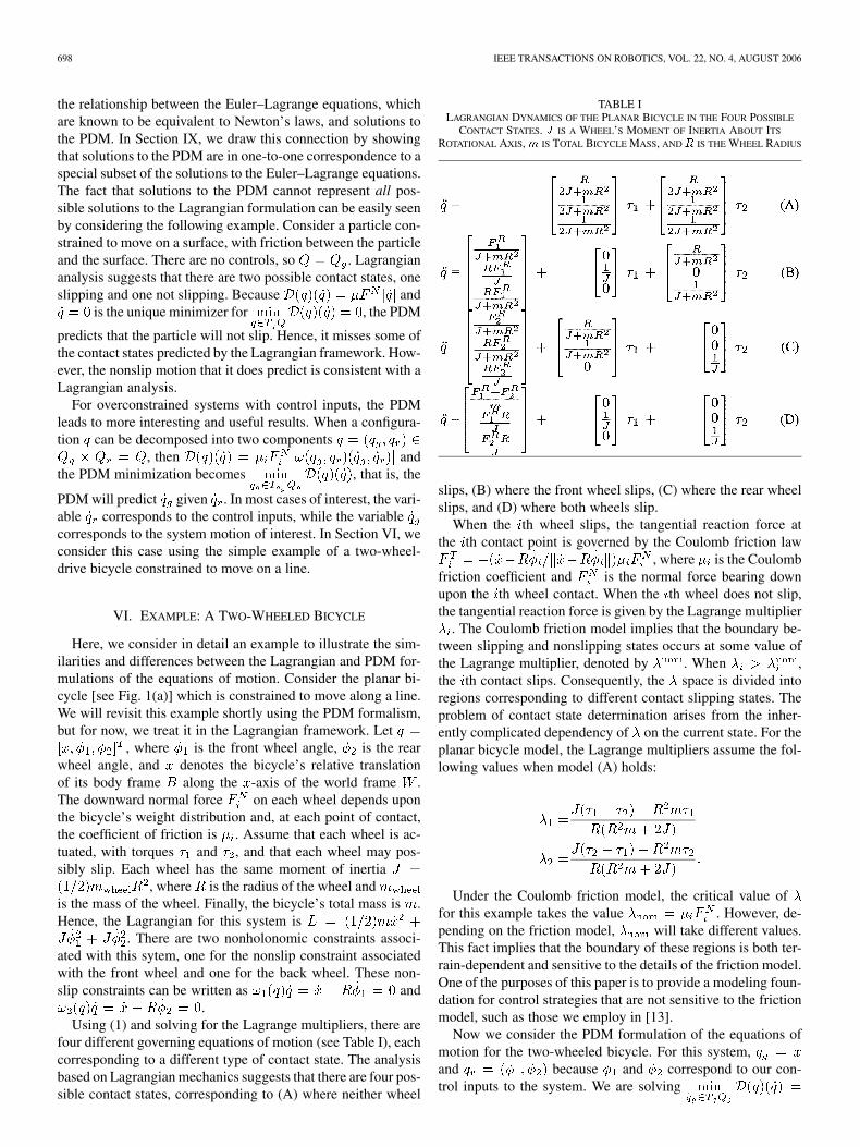
four different governing equations of motion (see Table I), eachcorresponding to a different type of contact state. The analysisbased on Lagrangian mechanics suggests that there are four pos-sible contact states, corresponding to (A) where neither wheel

TABLE ILAGRANGIAN DYNAMICS OF THE PLANAR BICYCLE IN THE FOUR POSSIBLE

CONTACT STATES. J IS A WHEEL’S MOMENT OF INERTIA ABOUT ITS

ROTATIONAL AXIS,m IS TOTAL BICYCLE MASS, ANDR IS THE WHEEL RADIUS

slips, (B) where the front wheel slips, (C) where the rear wheelslips, and (D) where both wheels slip.

When the th wheel slips, the tangential reaction force atthe th contact point is governed by the Coulomb friction law

, where is the Coulombfriction coefficient and is the normal force bearing downupon the th wheel contact. When the th wheel does not slip,the tangential reaction force is given by the Lagrange multiplier

. The Coulomb friction model implies that the boundary be-tween slipping and nonslipping states occurs at some value ofthe Lagrange multiplier, denoted by . When ,the th contact slips. Consequently, the space is divided intoregions corresponding to different contact slipping states. Theproblem of contact state determination arises from the inher-ently complicated dependency of on the current state. For theplanar bicycle model, the Lagrange multipliers assume the fol-lowing values when model (A) holds:

Under the Coulomb friction model, the critical value offor this example takes the value . However, de-pending on the friction model, will take different values.This fact implies that the boundary of these regions is both ter-rain-dependent and sensitive to the details of the friction model.One of the purposes of this paper is to provide a modeling foun-dation for control strategies that are not sensitive to the frictionmodel, such as those we employ in [13].

Now we consider the PDM formulation of the equations ofmotion for the two-wheeled bicycle. For this system,and because and correspond to our con-trol inputs to the system. We are solving


, which implies that

or . Hence, the equations of motion may bewritten as

(4)

where can change over time. Therefore, this is a multiple-model system as described in Definition 4.1. Note that when

, this minimization does not have a unique so-lution. In fact, all values in the convex hull of andminimize . We should add, however, that this same inde-terminate situation occurs in the Lagrangian dynamics when

at the th contact. Therefore, the PDM has onlytwo dynamic states, while the Lagrangian dynamics have four.We will see in Section IX that the two dynamic states comingfrom the PDM correspond to (B) and (C) in Table I. Moreover,they include (A) as a degenerate case (when , im-plying that ). Only (D) is not included in the PDMrepresentation.

In Section VII, we will turn to some of the more mathematicalproperties of the PDM that generalize some of our observationsabout the two-wheeled bicycle. In particular, we show that thePDM leads to multiple-model systems, and show that, in gen-eral, the model determination is unique, with only occassionaloccurance of indeterminant solutions.

VII. CHARACTERISTICS OF THE PDM

Here, we formalize the PDM and show that the PDM generi-cally gives rise to MMDA systems, as described in Section IV.Specifically, the PDM generically yields unique solutions, andwhen the equations of motion are not unique, they can still bebounded.

Before proceeding, let us recall a few facts that were alreadyestablished by Alexander and Maddocks [1]. They showed thatthe dissipation function of (3) is convex, so that its local minimaare also its global minima, should they exist. They also showthat, if such a minimum exists, it must exist at a point of nondif-ferentiability of due to the piecewise continuity of .

Let denote the constraint 1-forms. Forour purposes, these constraint 1-forms generally will representthe nonholonomic constraints associated with point contact.Furthermore, let consist of the velocitiesthat have the property that is a kinematicsolution to a nonoverconstrained subset consisting ofconstraints, i.e.,

...

It is straightforward to show that at least one minimizer ofmust ben an element of . See, for instance, [1] and [28]. Re-order so that . Al-though is associated with at least one of the minima achievedby , it does not necessarily contain all of them. In fact, ifmore than one element of is a minimum, then every elementof the convex hull of these minima are also minima. Hence, if

there is more than one solution, there are an infinite number ofsolutions.

Proposition 7.1: If and both minimize the dissipationfunctional found in Definition 5.1, then so does .

Proof: Assume and .Then

Moreover, equality must hold because we know that the min-imum is in . Therefore, the convex hull of and minimizes

. The proof for higher numbers of having equal dissipa-tion is by induction on this argument.

This result formalizes the intuition that if the power dissipatedis equal for two velocities , then all possible trajectories whosevelocity lies in the convex hull of the will satisfy the minimumalso; that is, in the nongeneric case when does not have aunique minimum, we can still bound the object’s motion. Let usconsider the extent to which the function having a uniqueminimum over is generic. We denote the function space ofthe coefficient of friction by and the function space of normalforces by . The following is a rephrasing of a result in [1]using the notation developed here.

Proposition 7.2: Assume : is ofthe form in Definition 5.1. Then, given , the dissipation func-tional almost always has a unique minimum with respectto (i.e., except on a set of measure zero1 relative to the space

).This result states that solving for equations of motion using

the PDM will almost always yield a unique solution. However,whenever the system is transitioning from one solution to an-other because of a change in or , the solution will becomea set instead of a singleton. This set is bounded by the elementsof that minimize . This makes the comment made in[1] rigorous, referring to the physical expectation of continuallyswitching back and forth between the dominance of one wheelor another, rather than staying in an indeterminate state. Propo-sition 7.2 additionally establishes a relationship between solu-tions that minimize and MMDA systems. Moreover, wewill see that the contact states predicted by the PDM arereductions of a class of mechanical control systems on .

1Intuitively, sets of measure zero can be as sparse as disjoint points in Q oras replete as a submanifold of Q. For example, consider a vehicle moving onsmooth terrain. In its ambient Euclidean space, a vehicle is always constrainedto a set of measure zero, yet that set is precisely where the interesting dynamicsoccur. On the other hand, sets of measure zero can represent arbitrary alge-braic relationships between parameters and the state space. Unless there is somereason to believe that these relationships are necessarily satisfied, we can feelphysically motivated in asserting they will not occur in practice. This is the casethat we are considering, and therefore, we feel that the ensuing results do implythe genericity we assert. Nevertheless, whether or not these sets are important inthe analysis is a physical assumption, not a mathematical result. For a referenceon measure theory, see [29].


Proposition 7.2 also implies that multiple-model systems area natural result of frictional interactions. Consequently, mul-tiple-model modeling and control techniques should be devel-oped for systems involving frictional contact. In Section IX, wewill explore more formally the relationship between solutions tothe PDM and solutions to the Lagrangian dynamics. However,before we can do that, we must explore in detail the notion ofkinematic reducibility for mechanical systems and how it canbe extended to multiple-model systems.

VIII. KINEMATIC REDUCIBILITY FOR

MULTIPLE-MODEL SYSTEMS

Here, we introduce the formal tools and results requiredto relate solutions arising from the PDM to solutions arisingfrom the full Lagrangian analysis. A rigorous understanding ofthe PDM’s properties and its relationship to conventional La-grangian mechanical analysis has heretofore been missing. Westructure our analysis of this issue in two steps. In the previoussection, we developed a more formal mathematical frameworkfor the PDM. In particular, we showed that the PDM leadsgenerically to multiple-model systems. This section introduceskinematic reducibility theory for multiple-model systems. Wethen use our multimodel reduction theory to formally study therelationship between the properties of the PDM solutions andthose of the associated Lagrangian models (in Section IX-B).

A. Review of Kinematic Reducibility for Smooth Systems

We briefly review the relevant notions of kinematic reductionhere, without going into detail on the underlying formalism. Forsome of these details, refer to the Appendix and to [7]. The no-tion of -reducibility formalizes what is meant by kine-matic reducibility. For mechanical systems, we consider inputs

: that are essentially bounded and Lebesgue inte-grable. In [7], it was assumed that inputs are absolutely contin-uous functions, since piecewise continuity implies that instanta-neous changes in system velocity are possible. In the presenceof inertial effects, such changes can only occur when infiniteforces are allowed. We keep this assumption on the inputs. How-ever, here state transitions are being approximated with piece-wise continuous signals. This is a common approximation inmany areas of physical modeling [30], such as impacting bodies.Therefore, we only require that absolute continuity hold locallyrather than globally.

Definition 8.1: : is absolutely continuous, iffor each such that for every finite collection

of nonoverlapping intervals in with theproperty that

we have

This definition implies that exists almost everywhere.Like [7], we restrict our attention to systems that can be

modeled as simple mechanical systems in a piecewise sense.In simple mechanical systems, the Lagrangian takes the form

. Assume that is an -dimensional configu-ration manifold, and is a Riemannian metric on definingthe kinetic energy. Since many of the applications of interest

are systems with no potential energy, let us simplify to the casewhere (i.e., ). Denote by elements in thetangent space of at , . With zero potential energy, thesystem Lagrangian takes the form .

Given a metric on the manifold , constraints modeled as1-forms in , and inputs , it is possible to show that theEuler–Lagrange dynamical equations can be written in the form

(5)

where is a path on and , andis the constrained affine connection associated with the metric(see the Appendix). Note that (5) is a second-order differentialequation evolving on the manifold . On the other hand, giveninput velocities , kinematic equations can be written in theform

(6)

Our goal is to formally reduce (5) to (6). Moreover, ifare kinematic vector fields and are dynamic vector fields,we let the distributions and be defined byspan and span . Relating these two sets ofvector fields will be of primary importance to us. Now, we saywhat we mean by a solution to a control system.

Definition 8.2: Let be a smooth control systemon a smooth manifold , and let . A

solution to is a pair , where : and: satisfy .

Note that Definition 8.2 only makes sense for first-order equa-tions evolving on , and (5) is a second-order differential equa-tion evolving on . Hence, we must rewrite (5) as a first-orderequation evolving on . To do this, we must introduce the ver-tical lift, defined by

(where is a vector field on ) and the geodesic spray, definedin coordinates by

where are the Christoffel symbols associated with (seethe Appendix). Let

denote the tangent bundle projection. Then, (5) written as a first-order system evolving on is

(7)

where . We now can define what it means for a me-chanical system of the form in (5) to be reducible to (6).


Definition 8.3: Let be an affine connection on (see theAppendix), and let and be two families of control functions.The system in (5) is -reducible to the system in (6) if thefollowing two conditions hold.

1) For each solution of the dynamic equation(5), with initial conditions in the distribution ,there exists a solution of the kinematic (6)with the property that .

2) For each solution of the kinematic (6), thereexists a solution of the dynamic (5), with theproperty that for almost every .

Condition 1) says that for every solution of a dynamic system,there must exist a kinematic solution that is the projection ofthe dynamic system. In the case of a vehicle, this correspondsto requiring that for every trajectory of the vehicle, there ex-ists a corresponding path that can be obtained from kinematicconsiderations alone. Condition 2) says that for every kinematicsolution, there must exist a dynamic solution that is equal to thekinematic solution coupled with its time derivative (so that itlies in ). This means that there must exist a dynamic solu-tion for every feasible kinematic path. We should point out herethat this is related to the classes of admissible inputs. Becausekinematic inputs must be essentially integrals of dynamic in-puts, they must be absolutely continuous if the dynamic inputsare integrable. Otherwise, infinite forces would be required (see[7]).

Let denote those vector fields taking values in adistribution . The following theorem states the local test for(5) to be , reducible to (6).

Theorem 8.1 [7]: Let be an affine connection, and letand be vector fields on a manifold .

The control system in (5) is -reducible to a system of theform in (6) if and only if (iff) the following two conditions hold.

1) span spanfor each (in particular, ).

2) for everywhere is the symmetric product of vector fields, de-fined in the Appendix.

This theorem says that if the input distributions of both thekinematic and dynamic systems are the same, and the dynamicsystem is closed under symmetric products, then the systemis kinematic. Some other things to note about kinematic re-ducibility include the following. First, all fully actuated sys-tems are automatically kinematically reducible, because theirdynamic input vector fields are always closed under symmetricproducts. For instance, the forward kinematics of a robotic ma-nipulator are kinematic whether moving in air (where the kine-matic approximation is obvious), or in a viscous fluid of somesort.

Note that kinematic reducibility is not the same thing as the“quasi-static” assumption commonly made in robotics. This isbecause kinematic reducibility only requires that there be a com-plete correspondence between dynamic motions and kinematicmotions. This implies that systems operating at high speedswith large forces can still be kinematic. On the other hand,quasi-static assumptions, when formalized at all, typically re-quire that the system be moving slowly in some sense, or tohave forces balance such that the net force is zero. We will see

that the quasi-static motions predicted by the PDM are indeedkinematic, but kinematic motions need not be quasi-static.

B. Main Result on Reducibility of Multiple-Model Systems

We now consider the problem of whether or not a dynamicmultiple-model system is kinematically reducible to an MMDAsystem. Lemma 8.2 states that if switches in system dynamicsare separated by a small amount of time (making the switchingsignal piecewise continuous), then the resulting solution is alsokinematically reducible.

Lemma 8.2: Let be a multiple-model system where theindividual model components are of the form in (5),and whose switching signal is piecewise constant. Then, is

-reducible iff the individual model componentsare all -reducible.

Proof: Since is piecewise constant, switches a count-able number of times. Therefore, let the times when changesits value be denoted for in some index set .Then, on the intervals , is -reducible, makingit -reducible almost always.2 It therefore satisfies the re-quirements of Definition 8.3.

We will use this lemma to prove Theorem 8.4, which says thatsolutions to the differential inclusion defined by multiple-modelsystems are kinematically reducible iff the individual models arekinematically reducible. Before proving that this is true, we willneed the following result from [31].

Theorem 8.3 [31]: Let : be acompact, set-valued map, and let be a sequence of solu-tions to the differential inclusion

(8)

such that . Then, is also a solution to (8).

Note that solutions to the differential inclusion are, in gen-eral, not unique, meaning that there is often an infinite familyof solutions. This theorem says that for a compact differentialinclusion, a converging sequence of solutions converges to asolution. Theorem 8.3 will be used several times in the proofof Theorem 8.4. Roughly speaking, piecewise continuous

-reducible solutions of the multiple-model mechanicalsystem can be used as approximations to flows of elements in ,where assumes the form of the right-hand side of (9). Theorem8.3 can then be used to show that their kinematic counterpartson must also converge to an element of the differentialinclusion defined on . This brings us to our main result.

Theorem 8.4: A multiple-model system where theindividual model components are of the formin (5) [or equivalently, the first-order form in (7)] is

-reducible iff the individual dynamical modelsare all -reducible.

Proof: First, note that it is obviously necessary that allof the individual models be -reducible in order for theresulting multiple-model system to be reducible. Otherwise, avalid solution to a multiple-model system is the smooth, nonre-ducible solution of one of the models in the set of models. Toshow sufficiency, we must show that when the individual models

2That is, it is reducible everywhere except for a set of measure zero.


are -reducible, all solutions to the MMDA system are-reducible. We show this in two steps. The first step con-

structs kinematic solutions given dynamic ones, and the secondstep constructs dynamic solutions given kinematic ones.

1) A multiple-model mechanical system has the form

(9)

where is the index for a given model, isthe metric appropriate to that model, is the affineconnection associated with the metric , and is thevector field representing the force input correspondingto of the th model of the multiple-model system. Incoordinates, (9) is equivalent to

(10)

where are the Christoffel symbols associated withthe metric . Expressed as a first-order system evolvingon in natural coordinates , these equa-tions take the form

Using these coordinates on , setand ,

with denoting the convex hull. In [31], itwas shown that solutions to a discontinuous systemcoincide with solutions of a differential inclusion of theconvex hull of the discontinuous system. Applying thisto our systems of interest, we see that solutions to amultiple-model system (viewed as a first-order systemon ) coincide with solutions to the differentialinclusion for , or in vector notation

(11)

Then, for a given solution of (11), we know that. Therefore, we can choose a selection

(an element) of , denoted , such thatlocally approximates the flow . Because is convex,we can rewrite a selection of as

(12)

for any such that and .Now we need to approximate solutions of the differen-tial inclusion in (11) using a piecewise constant . Let

be the flow of a smooth vector field for time .

Moreover, let . In [32],it was shown that we can choose the following map to

approximate (in the sense of pointwise convergence to aset) the flow of a selection :

(13)

Each of the component flows contributingto the flow consists of a flow along a -re-ducible mechanical system. Moreover, is a so-lution of (11) on , which is absolutely continuousfor every . This is due to the fact that we assume thatthe switching and forces are measurable, and that theLebesgue integral of measurable signals is absolutelycontinuous. This construction is useful because it allowsone to produce a solution (with piecewise constant)that approximates the flow along any selection of .More precisely, it converges to the flow of the selection

as ; that is, by applying Theorem 8.3 to theTaylor expansion of , we locally get

By assumption, we know that each segmentof is -reducible. Therefore, for every choiceof , is -reducible by Lemma 8.2. Theseresults then yield us, for each , a corresponding mapon

(14)

where . Here, eachis the flow of equations that are -reductions [asin (6)] from equations that generate the flow .Moreover, from Theorem 8.3, we know that

exists, and that its limit is a solution to

(15)

where , and the comefrom the reduced equations in (6). Therefore, part 1) ofDefinition 8.3 is satisfied.

2) The analysis of this second condition uses the same es-sential steps as above, but begins with the solution tothe kinematic equations and works towards a dynamicsolution. Starting with the solutions from (6), we knowthat for an individual model with index , we have

, or in vector form

(16)

Therefore, this MMDA system can be written in theform of (15). Again, for any given solution of (15),we have , so we can choose a selection

such that locally approximates the flow for


that solution. We can, moreover, construct a sequence ofsolutions converging to .

From Definition 8.3, we know we must show there exists ansolution with

By our construction, we know that

By assumption, for every and , there exists a corre-sponding such that . In thelimit

for some selection of the differential inclusion . Conse-quently, is a solution to (11), again by Theorem 8.3.Taking the derivative of both sides, we get

so part 2) is satisfied. This ends the proof.Notice that the proof of Theorem 8.4 relied heavily on specif-

ically constructing a solution with the desired properties basedon known solutions to the individual models comprising themultiple-model system. This result shows that determining thekinematic properties of the individual models in a multiple-model system is sufficient for determining the kinematic prop-erties of the entire system. Moreover, the transitions betweenmodels as the state evolves are also kinematic if the individualmodels are all kinematic.

IX. PDM AND -REDUCIBILITY

Here, we address the relationship between the models pro-duced by the PDM and the kinematically reducible states of ageneric mechanical system. An informal restatement of this isthe question: does the PDM produce equations of motion thatare kinematic reductions of Euler–Lagrange equations? First,we derive a result that will be shortly used to show the rela-tionship between PDM solutions and solutions of mechanical,second-order systems.

Proposition 9.1: Given a configuration manifold and a setof constraints which span the cotangent space , thenthe input distribution minimizing will always sat-isfy Null where is some collectionof which satisfy for .

Proof: Suppose that this was not the case. Then therewould exist , which minimizes such that, ifare the constraints which are satisfied, then Null and

. This implies that, for the choice of , stillminimizes . However, because the span , zero is

the unique minimizer, since is convex in . This contradictsthe assumption that and is a minimizer of .

This result roughly corresponds to the intuition that the min-imum dissipation in any unactuated direction is to not move atall in that direction. We should comment that this can still leadto a solution of no motion in the group variables; if the unactu-ated constraints dominate the motion, then the actuators will allslip.

Next, we consider the case where we are given a metric forsome mechanical system and a set of constraints described by1-forms . What are sufficient conditions for the resultingsystem to be -reducible? Lemma 9.2 gives one sufficientcondition which is invariant with respect to the metric , and isa simple corollary to the work found in [33] and [34].

Lemma 9.2: Given a “constraint distribution”which annihilates the constraints and an input distribution

, if , the mechanical system described byis -reducible.

Proof: Denote by the connection and by the con-strained connection defined by the Lagrange–dÁlembert prin-ciple (see the Appendix and [7] for details of this construction).We know that

and

which implies , .This, in turn, implies by Theorem 8.1 that is

-reducible.Therefore, -reducibility of a multiple-model mechan-

ical system is guaranteed regardless of the metric whenthe constraint distribution is equal to the input distribution.Moreover, we already know that the power-dissipation modelonly admits solutions where this is true. This allows us tointerpret the use of the PDM. The PDM is a way of choosing amore tractable subset of contact states from the full Lagrangiancontact mechanics. In other words, when we make the “kine-matic” assumption, we are merely restricting our attention to

-reducible systems. Moreover, when the reaction forcesdue to friction do not lie in , then those contact states arenot -reducible. However, we should be very clear thatthis only shows that the PDM captures -reducible stateswhen . That is, the correspondence only goesone direction: all PDM contact states are kinematic states, butnot all kinematic states can necessarily be predicted by thePDM. There are examples of mechanical systems which are

-reducible by virtue of properties of the metric . Forexamples of such systems, see [7].

In summary, we have shown the following.Theorem 9.3: Given a configuration manifold with tan-

gent space and constraints represented by 1-forms , thenall solutions to the PDM are -reductions of solutions toEuler–Lagrange equations on , constrained by a subset of

.We should also remark on the relationship between The-

orem 8.1 (reduction for smooth systems) and Theorem 8.4(reduction for multiple-model systems). In the smooth case,

-reducibility is equivalent to geodesic invariance (fordetails, see [7]). However, in the nonsmooth case, there is no


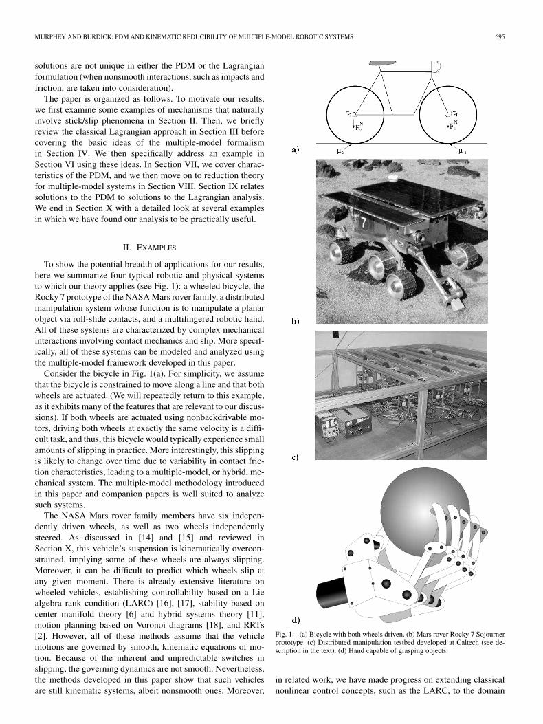
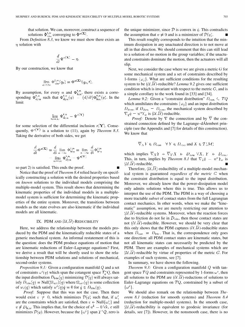
Fig. 2. Planar bicycle.

well-defined notion of geodesic invariance because the metricchanges over time. Nevertheless, we were able to extend thenotion of -reducibility relatively easily. Therefore, theconcept of -reducibility is, in some sense, more generalthan that of geodesic invariance.

X. EXAMPLES

To illustrate how the results presented in this paper are usefuland point towards more general applications of theories devel-oped here, we now revisit the examples from Section II. First,we come back to the bicycle example to illustrate all of thetheory details. We study the bicycle example in detail as il-lustration, and then quickly summarize several applications inother related work. For instance, we show how this analysishelps to establish controllability characteristics for the Marsrover family of vehicles and stability analysis for distributed ma-nipulation problems. We end this section with a brief discussionof how the method presented here can be applied to grasping andlocomotion.

A. Bicycle

Now, we return to the bicycle example of Section II (seeFig. 2) in detail. Assume that the bicycle is constrained to moveon a line. Recall that the bicycle has a total mass of , eachwheel has a moment of inertia and radius , and that the re-action forces are at the point of contact between the wheeland the ground. Using the mechanics formulation as describedin the Appendix, the configuration space is(where ), and the Riemannian metric describingthe kinetic energy is

The two nonrolling constraints are

and the constraint covectors can be written as

As inputs, we have

Now, for each combination of slipping and no slipping of thewheels, we have a set of equations to solve. Therefore, we havefour sets of equations to solve. Note that because the metric doesnot depend on the configuration, the Christoffel symbolsare all identically zero for this problem. Moreover, as we shallsee, the -orthogonal projection operator onto also doesnot depend on the configuration, indicating that the Christoffelsymbols for the constrained system [found in (26)] arealso identically zero. Therefore, the equations depend entirelyon the input forces and external forces due to friction.

1) No Slipping: When both wheels do not slip, both con-straints and are satisfied. This implies that the constraintdistribution is one-dimensional, spanned by

Moreover, one can compute that the -orthogonal complementof is

span

If we compute the -orthogonal projection onto the distribu-tion , we get

. The unprojected input vector fields are

Hence, the projected input vector fields are

and the equations of motion are therefore

It is easy to see that , so this is a kinematicsystem [i.e., it is reducible to (4)].

2) One Wheel Slipping: In the case where one wheel slips, wemay assume without loss of generality that the slipping wheelis wheel number 2. In this case, the constraint distribution is

Moreover, one can compute that the orthogonal complement ofis

To compute the reaction force due to the other wheel slipping,note that such a reaction force can be considered an externalforce, and can therefore be added to the right-hand side of (5),with the associated control assuming constant unity value


. If we compute the -orthogonal projection onto the distri-bution , we get

. The un-projected nominal inputs vector fields are the same as before

and the projected inputs vector fields are

The unprojected reaction force coming from the friction reac-tion force is

which, when projected onto the distribution , becomes

The equations of motion are therefore

To determine whether this system is kinematically reducible ornot, we first note that is again identically zero.Moreover, note that although Theorem 8.1 does not directly ad-dress the case of external forces, we can, by direct inspectionof Definition 8.3, see that if span , then the systemcannot, in general, be reducible. However, if span andthe satisfy the conditions for reducibility, then the systemis automatically reducible, because the external forces are “cov-ered” by the inputs. Therefore, we need only check that liesin the span of and . Indeed, span for this ex-ample. Therefore, this system is kinematically reducible. Notethat this property does not depend on the particular descriptionof the reaction force, and is, moreover, invariant with respect tothe reaction forces’ differentiability.

3) Both Wheels Slipping: When both wheels slip, there areno constraints to enforce. In this case, the constraint distributionis identically zero and the orthogonal complement is trivially theentire tangent space. Moreover, we can compute the reactionforce due to the wheels slipping to be and .The associated input vector fields and external vector fields are

and the equations of motion are therefore

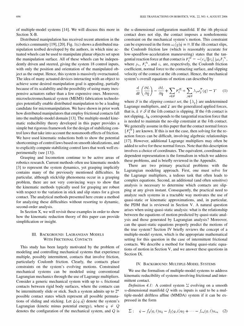
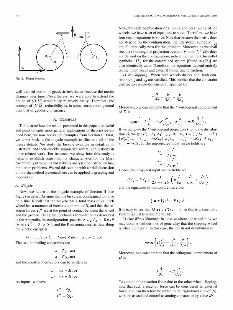
Fig. 3. Simplified Rocky 7: (a) Schematic of a six-wheeled rover.(b) Schematic of a simplification of the rover. The configuration of thisvehicle consists of the x, y, and � coordinates and the steering angle

(shown), as well as the three wheel angles (� ; � ; � ) (not shown).

In this case, it is clear that span . Therefore, thissystem (not surprisingly) is not kinematically reducible, at leastfor generic .

B. Simplified Mars Rover

Next, we revisit the example of Fig. 1(b), the geometry ofwhich we simplify here in Fig. 3 for the sake of discussion. Thissimplification has three wheels, with all three wheels driven.This model can be interpreted as a simplification of the Marsrover Rocky 7 vehicle, also seen in Fig. 1. The three-wheeled ve-hicle seen in the schematic has a configuration space consistingof . Hence,in this example, (the Special Euclidean group ofdistance preserving transformation in the plane) and(the four-dimensional input set). This system has six nonholo-nomic constraints (one associated with each wheel having both ano-roll constraint and a no-sideways-slip constraint). Therefore,there are possible models governing the dynamics ofthe vehicle. For this reason, we do not relate all of the calcula-tions for this vehicle. However, one can show, using a symbolicmathematics package such as Mathematica, that this system alsohas a subset of kinematic solutions, and that these solutions cor-respond to the the solutions to the PDM for this system. Onecan show that there only exist kinematic solutionsfor this system. Such a correspondence is important, becausethe PDM is very straightforward to solve, and these solutionscan be used for both controllability analysis and for purposes ofmotion planning (we have carried out this analysis in [14] and[15]).

In [14] and [15], we showed that this system’s controlla-bility properties can be analyzed using a set-valued extensionof the Lie bracket (the prerequisite calculation for understandingcontrollability using the classical LARC that arises naturally inMMDA analysis). Controllability is important for systems likethe Rocky 7, primarily because many motion-planning algo-rithms for vehicles are based on controllability properties. Forinstance, rapidly exploring random trees (RRTs) have been used


with much success to develop motion-planning strategies. How-ever, the computational intensity of these calculations is formi-dable, and recently [2] showed that significant advantage can betaken by reducing mechanical systems to kinematic ones whenusing RRTs for motion planning. Work is currently underwayto extend RRTs to the multiple-model systems of this paper.See [32] for a preliminary motion planning that is based on theMMDA structure found here.

We should comment on the relationship between kinematicreducibility results and controllability results which can be ob-tained for multiple-model systems [14], [15]. One of the intu-itive aspects of Theorem 8.4 is precisely that it is sufficient foreach model to be -reducible in order to guarantee thatthe multiple-model mechanical system is -reducible, i.e.,piecewise -reducibility is enough to guarantee -re-ducibility across discontinuities. However, in the case of con-trollability, this no longer holds. An MMDA system can switchamong individually controllable systems in such a way as to de-stroy controllability [15]. Thus, controllability of each model inan MMDA is not sufficient for overall controllability.

The fact that there is such a high number of models for theRocky 7 suggests the need for a reduction theory for multiple-model systems. Indeed, for a six-wheeled system like the actualRocky 7, there are possible models governing itsdynamics, which is a completely unmanageable number. For thethree-wheeled vehicle in the schematic, 20 kinematic models isalso perhaps an unreasonably large number of models to ana-lyze. In [15] we did an ad hoc reduction of this model, whichturned it into a two-model multiple-model system (although itcan be shown that no additional reduction is possible). Com-bining kinematic reduction with this multiple-model reductionreduced the number of models from 4096 to 2. Therefore, for-mally using reductions (both discrete and continuous) to reducethe dimensionality of the problem will be very useful, both formotion planning and estimation purposes. This will be a focusof future research.

C. Distributed Manipulation With Changing Contacts

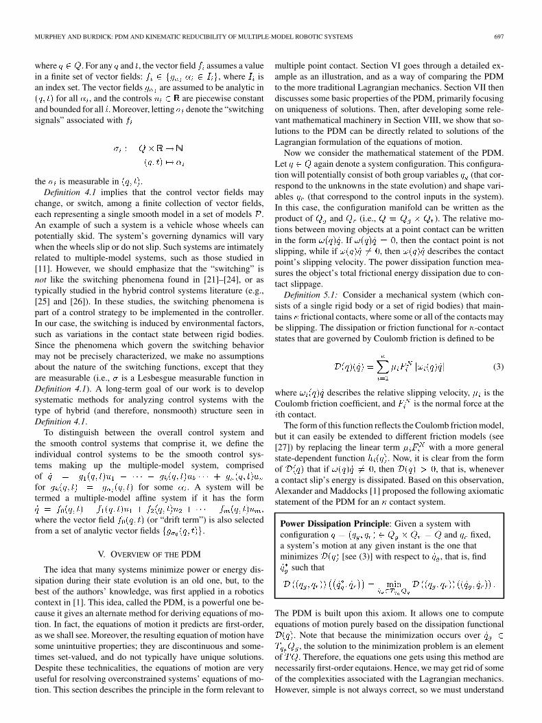
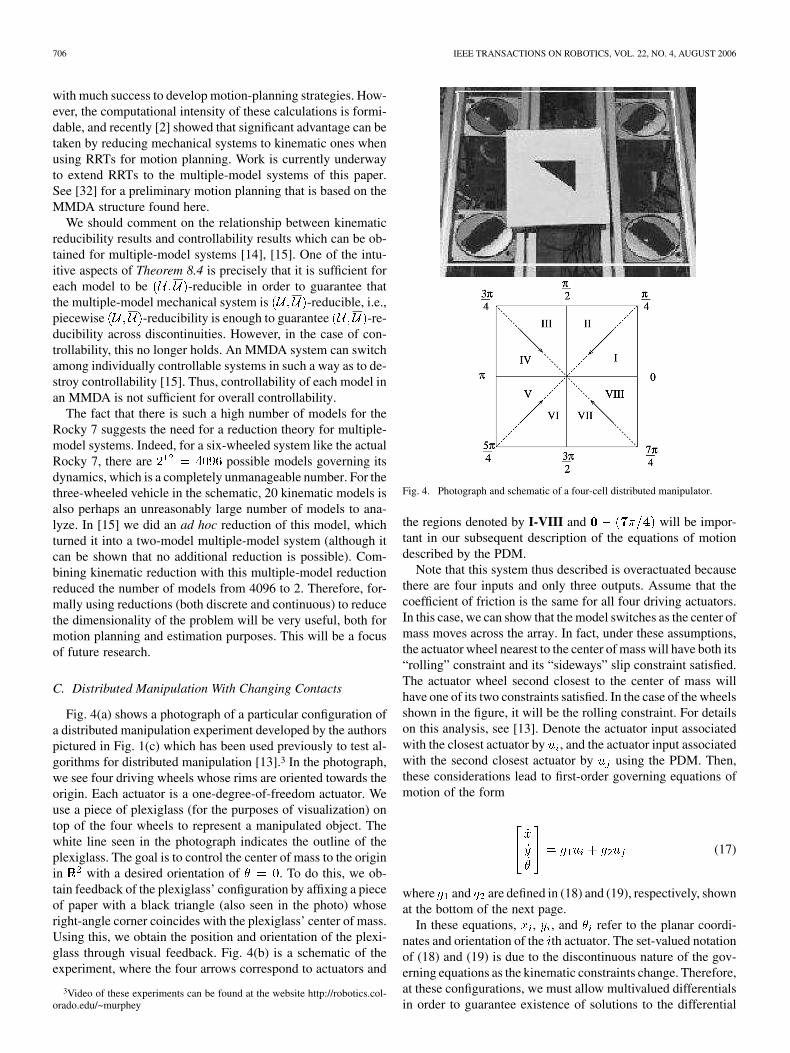
Fig. 4(a) shows a photograph of a particular configuration ofa distributed manipulation experiment developed by the authorspictured in Fig. 1(c) which has been used previously to test al-gorithms for distributed manipulation [13].3 In the photograph,we see four driving wheels whose rims are oriented towards theorigin. Each actuator is a one-degree-of-freedom actuator. Weuse a piece of plexiglass (for the purposes of visualization) ontop of the four wheels to represent a manipulated object. Thewhite line seen in the photograph indicates the outline of theplexiglass. The goal is to control the center of mass to the originin with a desired orientation of . To do this, we ob-tain feedback of the plexiglass’ configuration by affixing a pieceof paper with a black triangle (also seen in the photo) whoseright-angle corner coincides with the plexiglass’ center of mass.Using this, we obtain the position and orientation of the plexi-glass through visual feedback. Fig. 4(b) is a schematic of theexperiment, where the four arrows correspond to actuators and

3Video of these experiments can be found at the website http://robotics.col-orado.edu/~murphey

Fig. 4. Photograph and schematic of a four-cell distributed manipulator.

the regions denoted by I-VIII and will be impor-tant in our subsequent description of the equations of motiondescribed by the PDM.

Note that this system thus described is overactuated becausethere are four inputs and only three outputs. Assume that thecoefficient of friction is the same for all four driving actuators.In this case, we can show that the model switches as the center ofmass moves across the array. In fact, under these assumptions,the actuator wheel nearest to the center of mass will have both its“rolling” constraint and its “sideways” slip constraint satisfied.The actuator wheel second closest to the center of mass willhave one of its two constraints satisfied. In the case of the wheelsshown in the figure, it will be the rolling constraint. For detailson this analysis, see [13]. Denote the actuator input associatedwith the closest actuator by , and the actuator input associatedwith the second closest actuator by using the PDM. Then,these considerations lead to first-order governing equations ofmotion of the form

(17)

where and are defined in (18) and (19), respectively, shownat the bottom of the next page.

In these equations, , , and refer to the planar coordi-nates and orientation of the th actuator. The set-valued notationof (18) and (19) is due to the discontinuous nature of the gov-erning equations as the kinematic constraints change. Therefore,at these configurations, we must allow multivalued differentialsin order to guarantee existence of solutions to the differential


Fig. 5. Underactuated distributed manipulation feedback control.

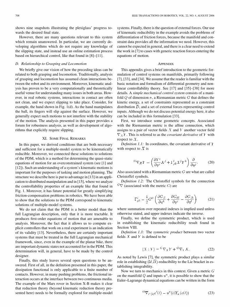
Fig. 6. Underactuated distributed manipulation movie snapshots. The goal is toalign the black triangle affixed to the plexiglass with the superimposed triangle.

equation in (17). It should be noted that here, the index notationshould be thought of as mapping pairs to equations of mo-tion in some neighborhood (not necessarily small) around theth and th actuators. In each region I-VIII, between the kine-

matics are smooth, but when a trajectory crosses a boundary, there is a discontinuity in the kinematics. It is pos-

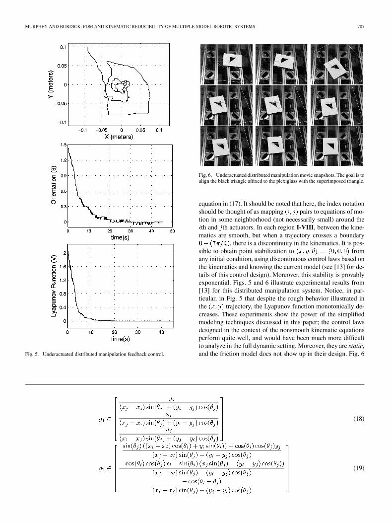
sible to obtain point stabilization to fromany initial condition, using discontinuous control laws based onthe kinematics and knowing the current model (see [13] for de-tails of this control design). Moreover, this stability is provablyexponential. Figs. 5 and 6 illustrate experimental results from[13] for this distributed manipulation system. Notice, in par-ticular, in Fig. 5 that despite the rough behavior illustrated inthe trajectory, the Lyapunov function monotonically de-creases. These experiments show the power of the simplifiedmodeling techniques discussed in this paper; the control lawsdesigned in the context of the nonsmooth kinematic equationsperform quite well, and would have been much more difficultto analyze in the full dynamic setting. Moreover, they are static,and the friction model does not show up in their design. Fig. 6

(18)

(19)


shows nine snapshots illustrating the plexiglass’ progress to-wards the desired final state.

However, there are many questions relevant to this systemwhich remain unanswered. In particular, we are currently de-veloping algorithms which do not require any knowledge ofthe slipping state, and instead use an online estimation processbased on hierarchical control, like that found in [8]–[11].

D. Relationship to Grasping and Locomotion

We briefly give our vision of how the preceding ideas can berelated to both grasping and locomotion. Traditionally, analysisof grasping and locomotion has assumed clean interactions be-tween the robot and its environment. Moreover, kinematic anal-ysis has proven to be a very computationally and theoreticallyuseful venue for understanding many issues in both areas. How-ever, in real robotic systems, interactions in contact are oftennot clean, and we expect slipping to take place. Consider, forexample, the hand shown in Fig. 1(d). As the hand manipulatesthe ball, its fingers will slip against the surface. However, wegenerally expect such motions to not interfere with the stabilityof the motion. The analysis presented in this paper provides aforum for robustness analysis, as well as development of algo-rithms that explicitly require slipping.

XI. SOME FINAL REMARKS

In this paper, we derived conditions that are both necessaryand sufficient for a multiple-model system to be kinematicallyreducible. Moreover, we connected these solutions to solutionsof the PDM, which is a method for determining the quasi-staticequations of motion for an overconstrained system (see [1] and[12]). Such an understanding of a system’s kinematic motions isimportant for the purposes of tasking and motion planning. Thestructure we describe here is put to advantage in [13] in an appli-cation to distributed manipulation and in [15], where we analyzethe controllability properties of an example like that found inFig. 1. Moreover, it has future potential for greatly simplifyingfriction-compensation problems in robotics. We have been ableto show that the solutions to the PDM correspond to kinematicsolutions of multiple-model systems.

We do not claim that the PDM is a better model than thefull Lagrangian description, only that it is more tractable. Itproduces first-order equations of motion that are amenable toanalysis. Moreover, the fact that it allows us to compute ex-plicit controllers that work on a real experiment is an indicationof its validity [13]. Nevertheless, there are certainly importantsystems that must be treated in the full Lagrangian mechanicalframework, since, even in the example of the planar bike, thereare important dynamic states not accounted for in the PDM. Thisdetermination will, in general, have to be made by the controldesigner.

Finally, this study leaves several open questions to be an-swered. First of all, in the definition presented in this paper, thedissipation functional is only applicable to a finite number ofcontacts. However, in many pushing problems, the frictional in-teraction occurs at the interface between two continuous media.The example of the Mars rover in Section X-B makes it clearthat reduction theory (beyond kinematic reduction theory pre-sented here) needs to be formally explored for multiple-model

systems. Finally, there is the question of external forces. Our useof kinematic reducibility in the example avoids the problems ofdifferentiation of friction forces, because the manifold and con-straint data provides all the information we need. However, thiscannot be expected in general, and there is a clear need to extendthe work in [7] to cases with generic reaction forces entering theequations of motion.

APPENDIX

This appendix gives a brief introduction to the geometric for-mulation of control systems on manifolds, primarily following[7], [33], and [34]. We assume that the reader is familiar with thebasic notation and formalism of differential geometry and non-linear controllability theory. See [17] and [35]–[38] for moredetails. A simple mechanical control system consists of a mani-fold of dimension , a Riemannian metric that defines thekinetic energy, a set of constraints represented as a constraintdistribution , and a set of external forces representing controlinputs. Although we do not discuss potential energy here, it alsocan be included in this formulation [33].

First, we introduce some geometric concepts. Associatedwith the Riemannian metric is the affine connection, whichassigns to a pair of vector fields and another vector field

. This is referred to as the covariant derivative of withrespect to .

Definition 1.1: In coordinates, the covariant derivative ofwith respect to is

(20)

Also associated with a Riemannian metric are what are calledChristoffel symbols.

Definition 1.2: The Christoffel symbols for the connection(associated with the metric ) are

(21)

where summation over repeated indexes is implied used unlessotherwise stated, and upper indexes indicate the inverse.

Finally, we define the symmetric product, which is usedin establishing the kinematic reducibility result found inSection VIII.

Definition 1.3: The symmetric product between two vectorfields and is defined to be

(22)

As noted by Lewis [7], the symmetric product plays a similarrole in establishing -reducibility to the Lie bracket in es-tablishing integrability.

Now we turn to mechanics in this context. Given a metricon the manifold and inputs , it is possible to show that theEuler–Lagrange dynamical equations can be written in the form

(23)


where is a path on and . Incoordinates, this is written as

(24)

Constrained systems, which are those control systems whosetrajectories must lie in some distribution , can also be de-scribed by (23). However, the affine connection must be mod-ified in order to incorporate the constraints. Let be a distri-bution on , and let denote the -orthogonal complementof . Moreover, let : be a -orthogonal projec-tion operator onto , and let : be a -orthogonalprojection onto . Last, let be any invertible (1,1) tensorfield on , and let be its inverse. Then, the Euler–Lagrangeequations can be written as (24), where the Chrisoffel symbolsare

where, again, is any invertible (1,1) tensor on . In orderto add forces, we must ensure the forces comply with the con-straints. Hence, the final equations of motion are

(25)

or in coordinates

(26)

Therefore, simple mechanical control systems all can be repre-sented using an affine connection. For more details and exam-ples worked out in detail, refer to [33].

REFERENCES

[1] J. Alexander and J. Maddocks, “On the kinematics of wheeled mobilerobots,” Int. J. Robot. Res., vol. 8, no. 5, pp. 15–27, Oct. 1989.

[2] P. Choudhury and K. Lynch, “Trajectory planning for kinematicallycontrollable underactuated mechanical systems,” in Algorithmic Foun-dations of Robotics V, ser. Springer Tracts in Advanced Robotics 7.Berlin, Germany: Springer-Verlag, 2004, pp. 559–575.

[3] B. Goodwine and J. Burdick, “Controllability of kinematic control sys-tems on stratified configuration spaces,” IEEE Trans. Autom. Control,vol. 46, no. 3, pp. 358–368, Mar. 2000.

[4] V. Kumar and J. Gardner, “Kinematics of redundantly actuated kine-matic chains,” IEEE J. Robot. Autom., vol. 6, no. 2, pp. 269–274, Apr.1990.

[5] R. Murray and S. Sastry, “Nonholonomic motion planning: Steeringusing sinusoids,” IEEE Trans. Autom. Control, vol. 38, no. 5, pp.700–716, May 1993.

[6] A. Teel, R. Murray, and G. Walsh, “Nonholonomic control systems:From steering to stabilization with sinusoids,” Int. J. Control, vol. 62,no. 4, pp. 849–870, 1995.

[7] A. Lewis, “When is a mechanical control system kinematic?,” in Proc.38th IEEE Conf. Decision Control, Dec. 1999, pp. 1162–1167.

[8] B. Anderson, T. Brinsmead, F. D. Bruyne, J. Hespanha, D. Liberzon,and A. Morse, “Multiple model adaptive control. I. Finite controllercoverings,” Int. J. Robust Nonlinear Control, vol. 10, George ZamesSpecial Issue, no. 11–12, pp. 909–929, Sep. 2000.

[9] J. Hespanha, D. Liberzon, A. Morse, B. Anderson, T. Brinsmead, andF. D. Bruyne, “Multiple model adaptive control. II. Switching,” Int.J. Robust Nonlinear Control , vol. 11, Special Issue on Hybrid Syst.Control, no. 5, pp. 479–496, Apr. 2001.

[10] J. Hespanha and A. S. Morse, “Stability of switched systems with av-erage dwell-time,” in Proc. IEEE Int. Conf. Decision Control, 1999,pp. 2655–2660.

[11] J. Hespanha, D. Liberzon, and A. Morse, “Logic-based switching con-trol of a nonholonomic system with parametric uncertainty,” Syst. Con-trol Lett., vol. 38, pp. 167–177, 1999.

[12] M. A. Peshkin and A. C. Sanderson, “Minimization of energy in qua-sistatic manipulation,” IEEE Trans. Robot. Autom., vol. 5, no. 1, pp.53–60, Feb. 1989.

[13] T. D. Murphey and J. W. Burdick, “Feedback control for distributedmanipulation with changing contacts,” Int. J. Robot. Res., vol. 23, no.7/8, pp. 763–782, Jul. 2004.

[14] ——, “A local controllability test for nonlinear multiple model sys-tems,” in Proc. IEEE Amer. Control Conf., Anchorage, AK, 2002, pp.4657–4661.

[15] ——, “Nonsmooth controllability and an example,” in Proc. IEEEConf. Decision Control, Washington, DC, 2002, pp. 370–376.

[16] I. Kolmanovsky and N. McClamroch, “Developments in nonholonomiccontrol problems,” IEEE Control Syst. Mag., pp. 20–36, Dec. 1995.

[17] R. Murray, Z. Li, and S. Sastry, A Mathematical Introduction to RoboticManipulation. Boca Raton, FL: CRC, 1994.

[18] H. Choset and J. Burdick, “Sensor-based exploration: The hierarchicalgeneralized Voronoi graph,” Int. J. Robot. Res., vol. 19, no. 2, pp.96–125, 2000.

[19] K. Böhringer and H. Choset, Eds., Distributed Manipulation. Nor-well, MA: Kluwer, 2000.

[20] J. Luntz, W. Messner, and H. Choset, “Distributed manipulation usingdiscrete actuator arrays,” Int. J. Robot. Res., vol. 20, no. 7, pp. 553–583,Jul. 2001.

[21] M. Branicky, “Multiple Lyapunov functions and other analysis toolsfor switched and hybrid systems,” IEEE Trans. Autom. Control, vol.43, no. 4, pp. 475–482, Apr. 1998.

[22] D. Liberzon and A. Morse, “Basic problems in stability and design ofswitched systems,” IEEE Control Syst. Mag., vol. 19, no. 5, pp. 59–70,1999.

[23] W. Dayawansa and C. Martin, “A converse Lyapunov theorem for aclass of dynamical systems which undergo switching,” IEEE Trans.Autom. Control, vol. 44, no. 4, pp. 751–760, Apr. 1999.

[24] M. Zefran and J. Burdick, “Design of switching controllers for systemswith changing dynamics,” in Proc. Conf. Decision Control, 1998, pp.2113–2118.

[25] G. Pappas, G. Laffierier, and S. Sastry, “Hierarchically consistentcontrol sytems,” IEEE Trans. Autom. Control, vol. 45, no. 6, pp.1144–1160, Jun. 2000.

[26] E. Asarin, O. Bournez, T. Dang, O. Maler, and A. Pneuli, “Effectivesynthesis of switching controllers for linear systems,” Proc. IEEE, vol.88, no. 7, pp. 1011–1025, Jul. 2000.

[27] H. Olsson, K. Astrom, C. C. de Wit, M. Gafvert, and P. Lischinsky,“Friction models and friction compensation,” Eur. J. Control, vol. 4,no. 3, pp. 176–195, 1998.

[28] F. Clarke, Optimization and Nonsmooth Analysis. Philadelphia, PA:SIAM, 1990.

[29] M. Adams and V. Guillemin, Measure Theory and Probability. Cam-bridge, MA: Birkhäuser, 1996.

[30] A. van der Schaft and H. Schumacher, An Introduction to Hybrid Dy-namical Systems, ser. Lecture Notes in Control and Information Sci-ences. Berlin, Germany: Springer-Verlag, 2000, vol. 251.

[31] A. Filippov, Differential Equations with Discontinuous Right-HandSides. Norwell, MA: Kluwer, 1988.

[32] T. D. Murphey and J. W. Burdick, “Issues in controllability and mo-tion planning for overconstrained wheeled vehicles,” in Proc. Int. Conf.Math. Theory Netw. Syst. (MTNS), Perpignan, France, 2000 [Online].Available: http://www.univ-perp.fr/mtns2000/.

[33] F. Bullo and A. Lewis, Geometric Control of Mechanical Systems, ser.#49 in Texts in Applied Mathematics. Berlin, Germany: Springer-Verlag, 2004.

[34] ——, “Low-order controllability and kinematic reductions for affineconnection control systems,” SIAM J. Control Optim., vol. 44, no. 3,pp. 885–908, 2005.

[35] S. Sastry, Nonlinear Systems: Analysis, Stability, and Con-trol. Berlin, Germany: Springer-Verlag, 1999.

[36] R. Abraham, J. Marsden, and T. Ratiu, Manifolds, Tensor Analysis, andApplications. Reading, MA: Addison-Wesley, 1988.


[37] W. Boothby, An Introduction to Differentiable Manifolds and Rie-mannian Geometry. New York: Academic, 1986.

[38] F. Warner, Foundations of Differentiable Manifolds and Lie Groups.Berlin, Germany: Springer-Verlag, 1971.

Todd D. Murphey (M’01) received the B.S. degreein mathematics from the University of Arizona,Tucson, in 1997, and the Ph.D. degree in control anddynamical systems from the California Institute ofTechnology, Pasadena, in 2002.

He has been an Assistant Professor with the De-partment of Electrical and Computer Engineering,University of Colorado, Boulder, since 2004. Hiscurrent research interests include robotics, symbolicdynamics, the role of uncertainty in cooperating sys-tems, and friction-dominated mechanical systems.

Joel W. Burdick (M’95) received the B.S. degreefrom Duke University, Durham, NC, in 1981, and theM.S. and Ph.D. degrees from Stanford University,Stanford, CA, in 1982 and 1988, respectively, all inmechanical engineering.

Since 1988, he has been with the Division of En-gineering and Applied Science, California Instituteof Technology, Pasadena, where he is currently aProfessor with the Departments of Mechanical En-gineering and BioEngineering. His current researchinterests include robotic manipulation, sensor-based

motion planning, neural prosthetics, and rehabilitation of spinal cord injuries.

Date post:	22-Jul-2018
Category:	Documents
Upload:	truongkhanh
View:	214 times
Download:	0 times

694 IEEE TRANSACTIONS ON ROBOTICS, VOL. 22, NO....

Documents