7-1

Probabilistic Robotics: Kalman Filters

Slide credits: Wolfram Burgard, Dieter Fox, Cyrill Stachniss, Giorgio Grisetti, Maren Bennewitz, Christian Plagemann, Dirk Haehnel, Mike Montemerlo, Nick Roy, Kai Arras, Patrick Pfaff and others

Sebastian Thrun & Alex TeichmanStanford Artificial Intelligence Lab

7-2

Bayes Filters in Localization

111 )(),|()|()( tttttttt dxxBelxuxPxzPxBel

• Prediction

• Measurement Update

Bayes Filter Reminder

111 )(),|()( tttttt dxxbelxuxpxbel

)()|()( tttt xbelxzpxbel

Gaussians

2

2)(

2

1

2

2

1)(

:),(~)(

x

exp

Nxp

-s s

m

Univariate

)()(2

1

2/12/

1

)2(

1)(

:)(~)(

μxΣμx

Σx

Σμx

t

ep

,Νp

d

m

Multivariate

),(~),(~ 22

2

abaNYbaXY

NX

Properties of Gaussians

22

21

222

21

21

122

21

22

212222

2111 1

,~)()(),(~

),(~

NXpXpNX

NX

• We stay in the “Gaussian world” as long as we start with Gaussians and perform only linear transformations.

),(~),(~ TAABANY

BAXY

NX

Multivariate Gaussians

€

X1 ~ N(μ1,Σ1)

X2 ~ N(μ2,Σ2)

⎫ ⎬ ⎭⇒ p(X1) ⋅ p(X2) ~ N

Σ1−1

Σ1−1 + Σ2

−1μ1 +

Σ2−1

Σ1−1 + Σ2

−1μ2,

1

Σ1−1 + Σ2

−1

⎛

⎝ ⎜

⎞

⎠ ⎟

7-7

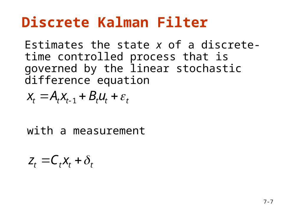
Discrete Kalman Filter

tttttt uBxAx 1

tttt xCz

Estimates the state x of a discrete-time controlled process that is governed by the linear stochastic difference equation

with a measurement

7-8

Components of a Kalman Filter

t

Matrix (nxn) that describes how the state evolves from t to t-1 without controls or noise.

tA

Matrix (nxl) that describes how the control ut changes the state from t to t-1.tB

Matrix (kxn) that describes how to map the state xt to an observation zt.tC

t

Random variables representing the process and measurement noise that are assumed to be independent and normally distributed with covariance Rt and Qt respectively.

7-9

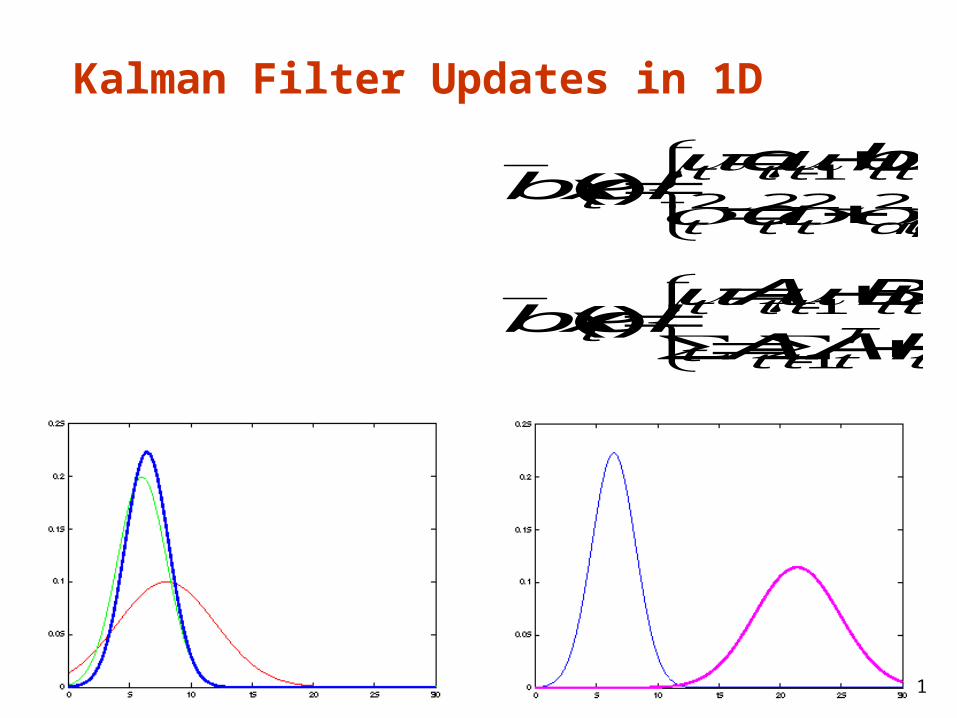
Kalman Filter Updates in 1D

7-10

Kalman Filter Updates in 1D

1)(with )(

)()(

tTttt

Tttt

tttt

ttttttt QCCCK

CKI

CzKxbel

2,

2

2

22 with )1(

)()(

tobst

tt

ttt

tttttt K

K

zKxbel

Kalman Filter Updates in 1D

tTtttt

tttttt RAA

uBAxbel

1

1)(

2

,2221)(

tactttt

tttttt a

ubaxbel

Kalman Filter Updates

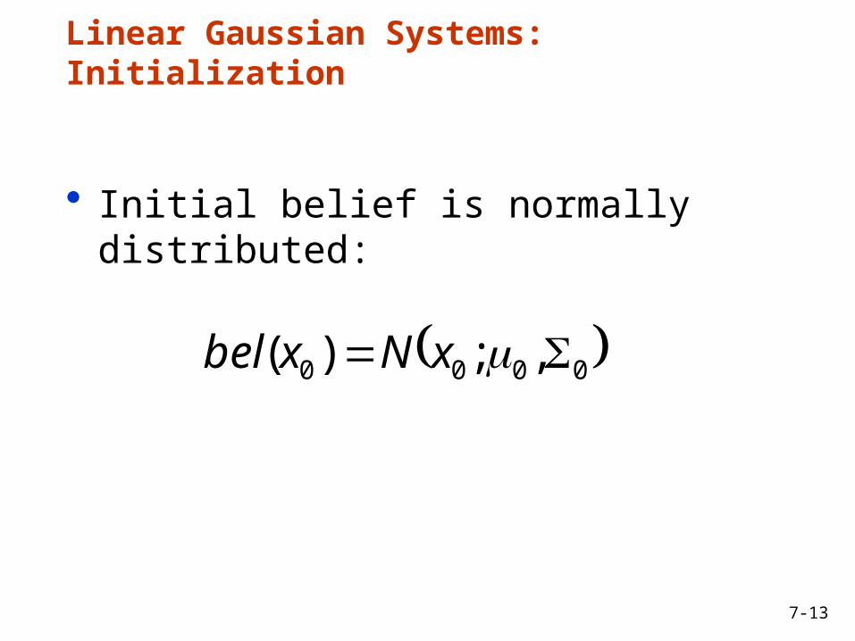
0000 ,;)( xNxbel

Linear Gaussian Systems: Initialization

• Initial belief is normally distributed:

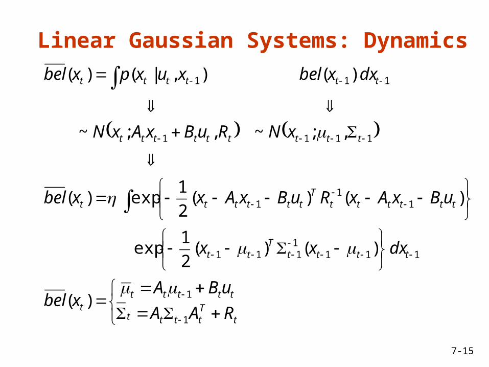
• Dynamics are linear function of state and control plus additive noise:

tttttt uBxAx 1

Linear Gaussian Systems: Dynamics

ttttttttt RuBxAxNxuxp ,;),|( 11

1111

111

,;~,;~

)(),|()(

ttttttttt

tttttt

xNRuBxAxN

dxxbelxuxpxbel

Linear Gaussian Systems: Dynamics

tTtttt

tttttt

ttttT

tt

ttttttT

tttttt

ttttttttt

tttttt

RAA

uBAxbel

dxxx

uBxAxRuBxAxxbel

xNRuBxAxN

dxxbelxuxpxbel

1

1

1111111

11

1

1111

111

)(

)()(2

1exp

)()(2

1exp)(

,;~,;~

)(),|()(

• Observations are linear function of state plus additive noise:

tttt xCz

Linear Gaussian Systems: Observations

tttttt QxCzNxzp ,;)|(

ttttttt

tttt

xNQxCzN

xbelxzpxbel

,;~,;~

)()|()(

Linear Gaussian Systems: Observations

1

11

)(with )(

)()(

)()(2

1exp)()(

2

1exp)(

,;~,;~

)()|()(

tTttt

Tttt

tttt

ttttttt

tttT

ttttttT

tttt

ttttttt

tttt

QCCCKCKI

CzKxbel

xxxCzQxCzxbel

xNQxCzN

xbelxzpxbel

Kalman Filter Algorithm

1. Algorithm Kalman_filter( mt-1, St-1, ut, zt):

2. Prediction:3. 4.

5. Correction:6. 7. 8.

9. Return mt, St

ttttt uBA 1

tTtttt RAA 1

1)( tTttt

Tttt QCCCK

)( tttttt CzK

tttt CKI )(

Kalman Filter Algorithm

Kalman Filter Algorithm

• Prediction• Observation

• Matching• Correction

7-21

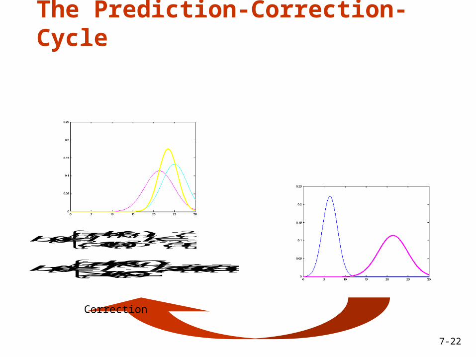
The Prediction-Correction-Cycle

tTtttt

tttttt RAA

uBAxbel

1

1)(

2

,2221)(

tactttt

tttttt a

ubaxbel

Prediction

7-22

The Prediction-Correction-Cycle

1)(,)(

)()(

tTttt

Tttt

tttt

ttttttt QCCCK

CKI

CzKxbel

2,

2

2

22 ,)1(

)()(

tobst

tt

ttt

tttttt K

K

zKxbel

Correction

7-23

The Prediction-Correction-Cycle

1)(,)(

)()(

tTttt

Tttt

tttt

ttttttt QCCCK

CKI

CzKxbel

2,

2

2

22 ,)1(

)()(

tobst

tt

ttt

tttttt K

K

zKxbel

tTtttt

tttttt RAA

uBAxbel

1

1)(

2

,2221)(

tactttt

tttttt a

ubaxbel

Correction

Prediction

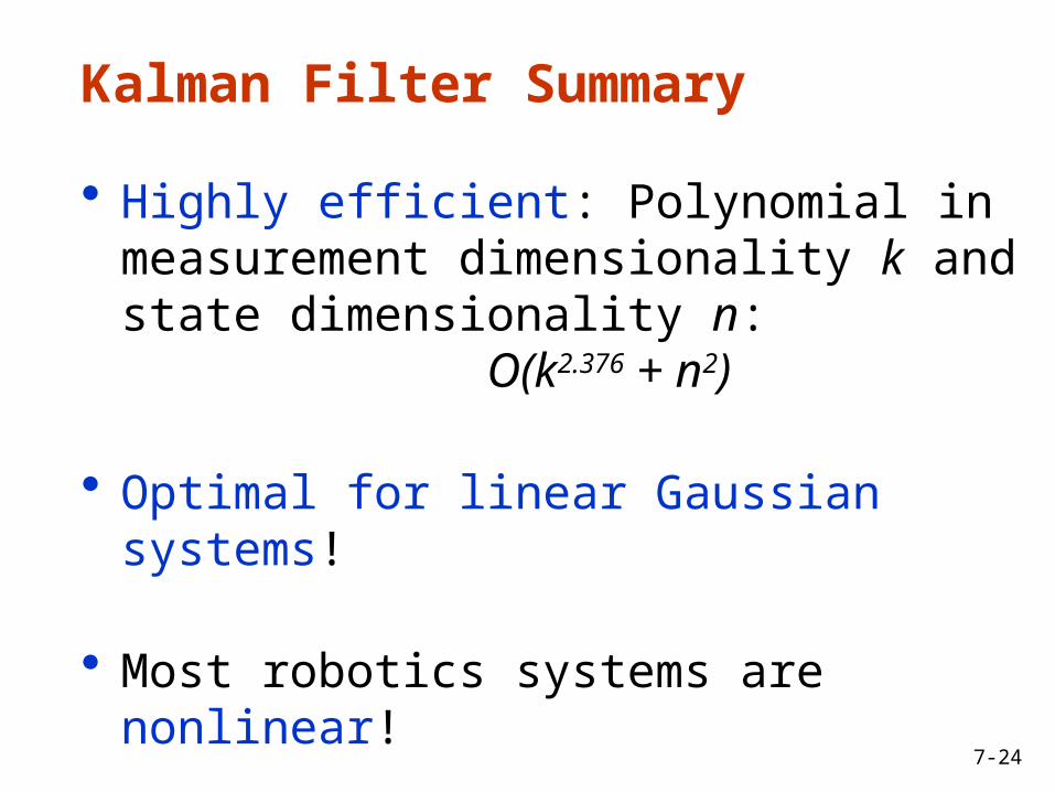
Kalman Filter Summary

• Highly efficient: Polynomial in measurement dimensionality k and state dimensionality n: O(k2.376 + n2)

• Optimal for linear Gaussian systems!

• Most robotics systems are nonlinear!

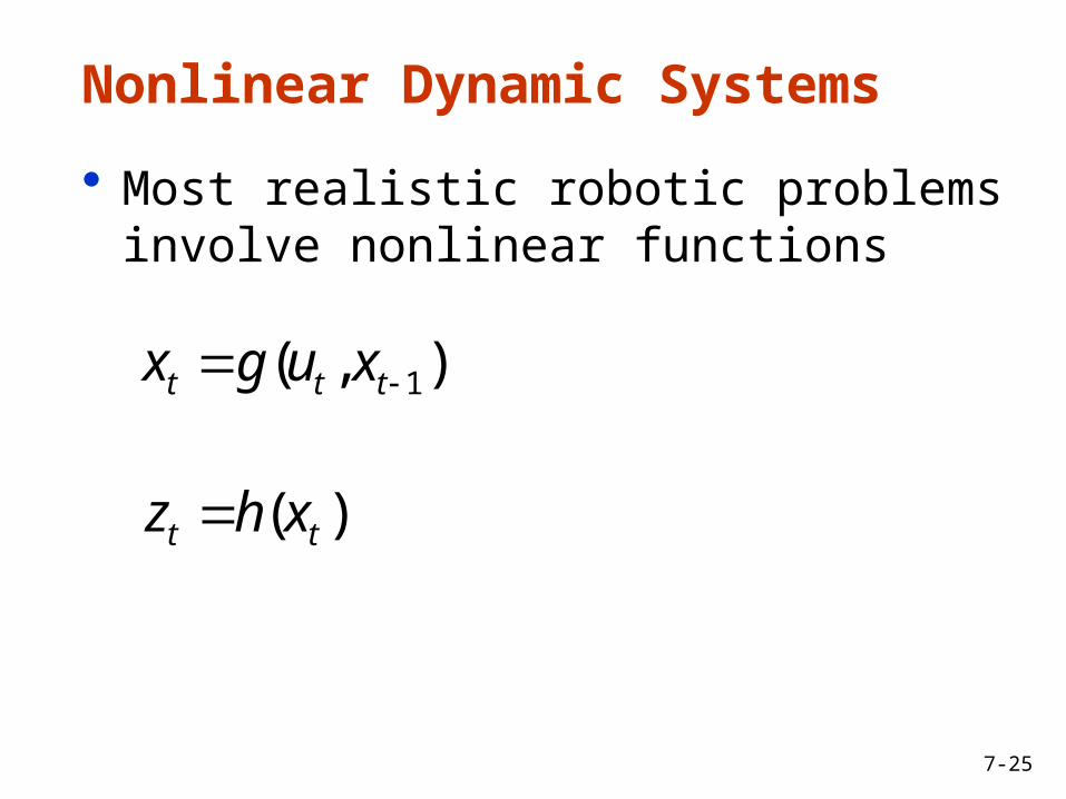
Nonlinear Dynamic Systems

• Most realistic robotic problems involve nonlinear functions

),( 1 ttt xugx

)( tt xhz

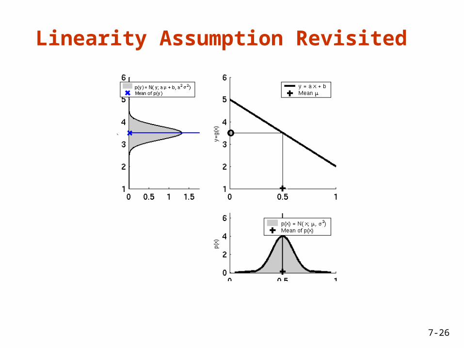
Linearity Assumption Revisited

Non-linear Function

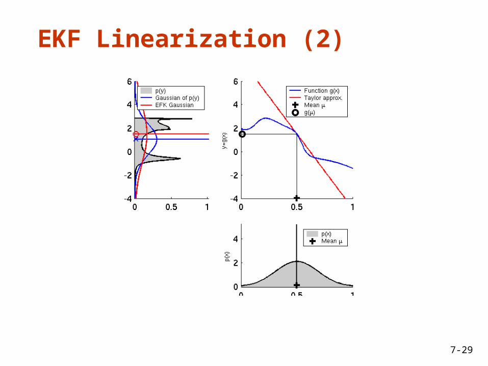
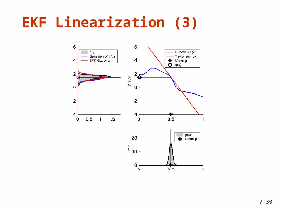
EKF Linearization (1)

EKF Linearization (2)

EKF Linearization (3)

• Prediction:

• Correction:

EKF Linearization: First Order Taylor Series Expansion

)(),(),(

)(),(

),(),(

1111

111

111

ttttttt

ttt

tttttt

xGugxug

xx

ugugxug

)()()(

)()(

)()(

ttttt

ttt

ttt

xHhxh

xx

hhxh

EKF Algorithm

1. Extended_Kalman_filter( mt-1, St-1, ut, zt):

2. Prediction:3. 4.

5. Correction:6. 7. 8.

9. Return mt, St

),( 1 ttt ug

tTtttt RGG 1

1)( tTttt

Tttt QHHHK

))(( ttttt hzK

tttt HKI )(

1

1),(

t

ttt x

ugG

t

tt x

hH

)(

ttttt uBA 1

tTtttt RAA 1

1)( tTttt

Tttt QCCCK

)( tttttt CzK

tttt CKI )(

Localization

• Given • Map of the environment.• Sequence of sensor measurements.

• Wanted• Estimate of the robot’s position.

• Problem classes• Position tracking• Global localization• Kidnapped robot problem (recovery)

“Using sensory information to locate the robot in its environment is the most fundamental problem to providing a mobile robot with autonomous capabilities.” [Cox ’91]

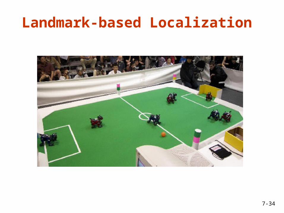
Landmark-based Localization

1. EKF_localization ( mt-1, St-1, ut, zt, m):

Prediction:

2.

3.

4. ),( 1 ttt ug

Tttt

Ttttt VMVGG 1

,1,1,1

,1,1,1

,1,1,1

1

1

'''

'''

'''

),(

tytxt

tytxt

tytxt

t

ttt

yyy

xxx

x

ugG

tt

tt

tt

t

ttt

v

y

v

y

x

v

x

u

ugV

''

''

''

),( 1

2

43

221

||||0

0||||

tt

ttt

v

vM

Motion noise

Jacobian of g w.r.t location

Predicted mean

Predicted covariance

Jacobian of g w.r.t control

1. EKF_localization ( mt-1, St-1, ut, zt, m):

Correction:

2.

3.

4.

5.

6.

)ˆ( ttttt zzK

tttt HKI

,

,

,

,

,

,),(

t

t

t

t

yt

t

yt

t

xt

t

xt

t

t

tt

rrr

x

mhH

,,,

2,

2,

,2atanˆ

txtxyty

ytyxtxt

mm

mmz

tTtttt QHHS

1 tTttt SHK

2

2

0

0

r

rtQ

Predicted measurement mean

Pred. measurement covariance

Kalman gain

Updated mean

Updated covariance

Jacobian of h w.r.t location

EKF Prediction Step

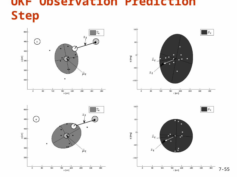
EKF Observation Prediction Step

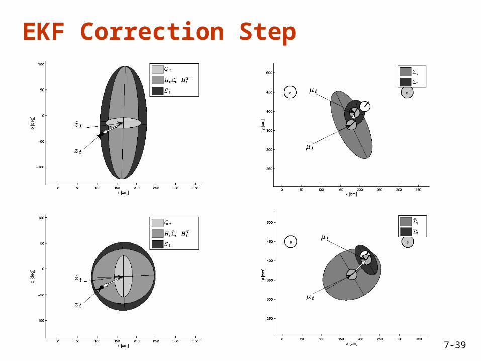
EKF Correction Step

Estimation Sequence (1)

Estimation Sequence (2)

Comparison to GroundTruth

EKF Summary

• Highly efficient: Polynomial in measurement dimensionality k and state dimensionality n: O(k2.376 + n2)

• Not optimal!• Can diverge if nonlinearities are large!• Works surprisingly well even when all

assumptions are violated!

EKF Localization Example

• Line and point landmarks

EKF Localization Example

• Line and point landmarks

EKF Localization Example

• Lines only (Swiss National Exhibition Expo.02)

Linearization via Unscented Transform

EKF UKF

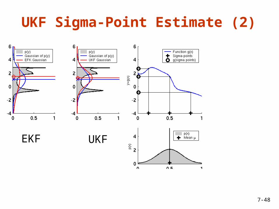
UKF Sigma-Point Estimate (2)

EKF UKF

UKF Sigma-Point Estimate (3)

EKF UKF

Unscented Transform

nin

wwn

nw

nw

ic

imi

i

cm

2,...,1for )(2

1 )(

)1( 2000

Sigma points Weights

)( ii g

n

i

Tiiic

n

i

iim

w

w

2

0

2

0

))(('

'

Pass sigma points through nonlinear function

Recover mean and covariance

UKF_localization ( mt-1, St-1, ut, zt, m):

Prediction:

2

43

221

||||0

0||||

tt

ttt

v

vM

2

2

0

0

r

rtQ

TTTt

at 000011

t

t

tat

Q

M

00

00

001

1

at

at

at

at

at

at 111111

xt

utt

xt ug 1,

L

i

T

txtit

xti

ict w

2

0,,

L

i

xti

imt w

2

0,

Motion noise

Measurement noise

Augmented state mean

Augmented covariance

Sigma points

Prediction of sigma points

Predicted mean

Predicted covariance

UKF_localization ( mt-1, St-1, ut, zt, m):

Correction:

zt

xtt h

L

iti

imt wz

2

0,ˆ

Measurement sigma points

Predicted measurement mean

Pred. measurement covariance

Cross-covariance

Kalman gain

Updated mean

Updated covariance

Ttti

L

itti

ict zzwS ˆˆ ,

2

0,

Ttti

L

it

xti

ic

zxt zw ˆ,

2

0,

,

1, tzx

tt SK

)ˆ( ttttt zzK

Tttttt KSK

1. EKF_localization ( mt-1, St-1, ut, zt, m):

Correction:

2.

3.

4.

5.

6.

)ˆ( ttttt zzK

tttt HKI

,

,

,

,

,

,),(

t

t

t

t

yt

t

yt

t

xt

t

xt

t

t

tt

rrr

x

mhH

,,,

2,

2,

,2atanˆ

txtxyty

ytyxtxt

mm

mmz

tTtttt QHHS

1 tTttt SHK

2

2

0

0

r

rtQ

Predicted measurement mean

Pred. measurement covariance

Kalman gain

Updated mean

Updated covariance

Jacobian of h w.r.t location

UKF Prediction Step

UKF Observation Prediction Step

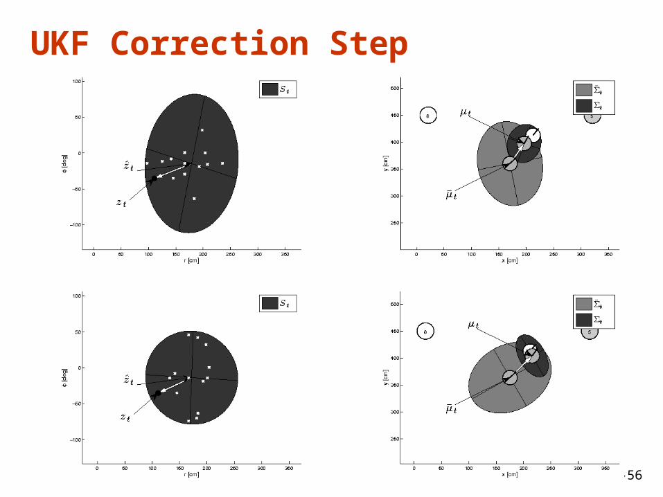
UKF Correction Step

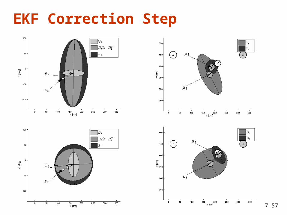
EKF Correction Step

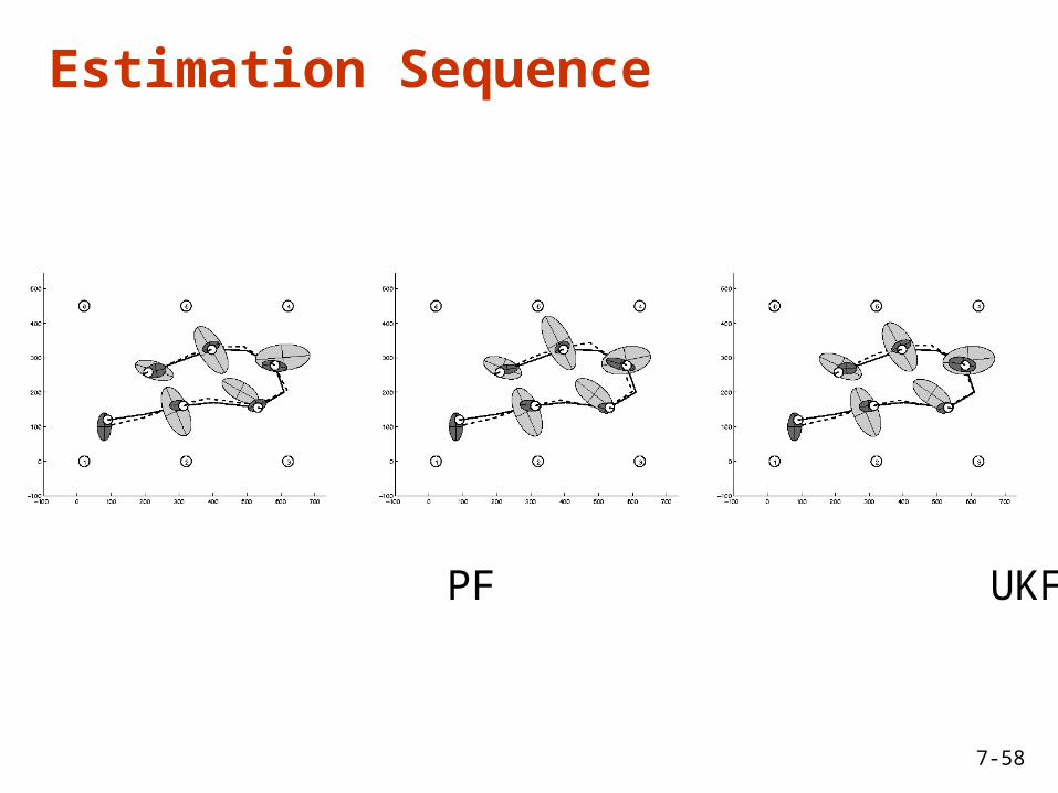
Estimation Sequence

EKF PF UKF

Estimation Sequence

EKF UKF

Prediction Quality

EKF UKF

7-61

UKF Summary

• Highly efficient: Same complexity as EKF, with a constant factor slower in typical practical applications

• Better linearization than EKF: Accurate in first two terms of Taylor expansion (EKF only first term)

• Derivative-free: No Jacobians needed

• Still not optimal!

• [Arras et al. 98]:

• Laser range-finder and vision

• High precision (<1cm accuracy)

Kalman Filter-based System

Courtesy of K. Arras

Multi-hypothesisTracking

• Belief is represented by multiple hypotheses

• Each hypothesis is tracked by a Kalman filter

• Additional problems:

• Data association: Which observation

corresponds to which hypothesis?

• Hypothesis management: When to add / delete

hypotheses?

• Huge body of literature on target tracking, motion

correspondence etc.

Localization With MHT

• Hypotheses are extracted from LRF scans• Each hypothesis has probability of being the correct

one:

• Hypothesis probability is computed using Bayes’ rule

• Hypotheses with low probability are deleted.

• New candidates are extracted from LRF scans.

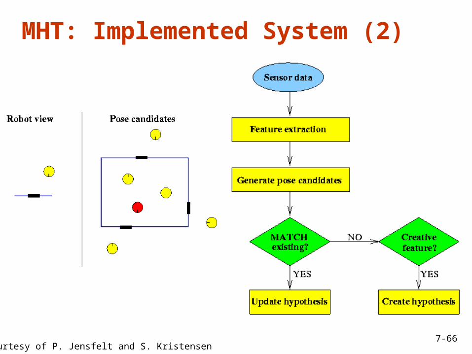
MHT: Implemented System (1)

)}(,,ˆ{ iiii HPxH

},{ jjj RzC

)(

)()|()|(

sP

HPHsPsHP ii

i

[Jensfelt et al. ’00]

MHT: Implemented System (2)

Courtesy of P. Jensfelt and S. Kristensen

MHT: Implemented System (3)Example run

Map and trajectory

# hypotheses

#hypotheses vs. time

P(Hbest)

Courtesy of P. Jensfelt and S. Kristensen

7-68

Summary: Kalman Filter

• Gaussian Posterior, Gaussian Noise, efficient when applicable

• KF: Motion, Sensing = linear• EKF: nonlinear, uses Taylor expansion• UKF: nonlinear, uses sampling• MHKF: Combines best of Kalman

Filters and particle filters

• A little challenging to implement