195 7 Introduction to Maple Programming Chemical engineers apply principles of chemistry, physics, and engineering to the design and oper- ation of industrial plants for the production of materials that are mixed and undergo other chemical changes during the manufacturing process. Reactors and reactor models can be used to synthesize and analyze the components that are combined to create products such as shampoos, cosmetics, plastics and drugs. The reactor model developed in this chapter’s application is based on the principle of conservation of mass. The use of Maple in the analysis of this model involves a user-defined procedure written in the Maple programming language. In addition to introducing the Maple programming language, you will find discussions on the use of conditional and looping statements. Solvents and Solutes
Transcript
195
7
Introduction to Maple Programming
C
hemical engineers apply
principles of chemistry, physics, and engineering to the design and oper-
ation of industrial plants for the production of materials that are mixed
and undergo other chemical changes during the manufacturing process.
Reactors and reactor models can be used to synthesize and analyze the
components that are combined to create products such as shampoos,
cosmetics, plastics and drugs. The reactor model developed in this
chapter’s application is based on the principle of
conservation of mass
.
The use of Maple in the analysis of this model involves a user-defined
procedure written in the Maple programming language. In addition to
introducing the Maple programming language, you will find discussions
on the use of conditional and looping statements.
Solvents and Solutes
196
MAPLE V FOR ENGINEERS
he first six chapters presented techniques for direct interactionwith Maple: enter a command, receive a response. While this is suf-ficient for many situations, there are times when repeatedly step-
ping through complicated multi-command sequences is inconvenient andinefficient. The main topic of this chapter is the use of Maple as a pro-gramming language to create user-defined commands, including loops,conditionals, input arguments, error handling, and return values.
The simplicity of Maple programs, more properly called
procedures
, isderived from the fact that the programming is done using standard Maplecommands. The power of the Maple programming language is evidencedby the fact that almost all Maple commands are implemented in the Mapleprogramming language. Moreover, as you will learn in Section 7.1, the def-initions can be viewed, and even modified, by the user.
Some of the examples and problems present a final look at examples andapplications from previous chapters. The application introduced in thischapter investigates some of the analytical techniques used by chemicalengineers in the design of reactors for the mixing of solvents and solutes.
7-1 VIEWING MAPLE PROCEDURES
Almost all Maple commands are written in Maple, and these definitionscan be viewed by the user. Thus, a natural way to begin to learn about theMaple programming language is by looking at the way these commandsare implemented. The
showstat
command (which is new in Release 4) dis-plays a procedure in a format that clearly illustrates the structure of theprocedure specified in the first argument.
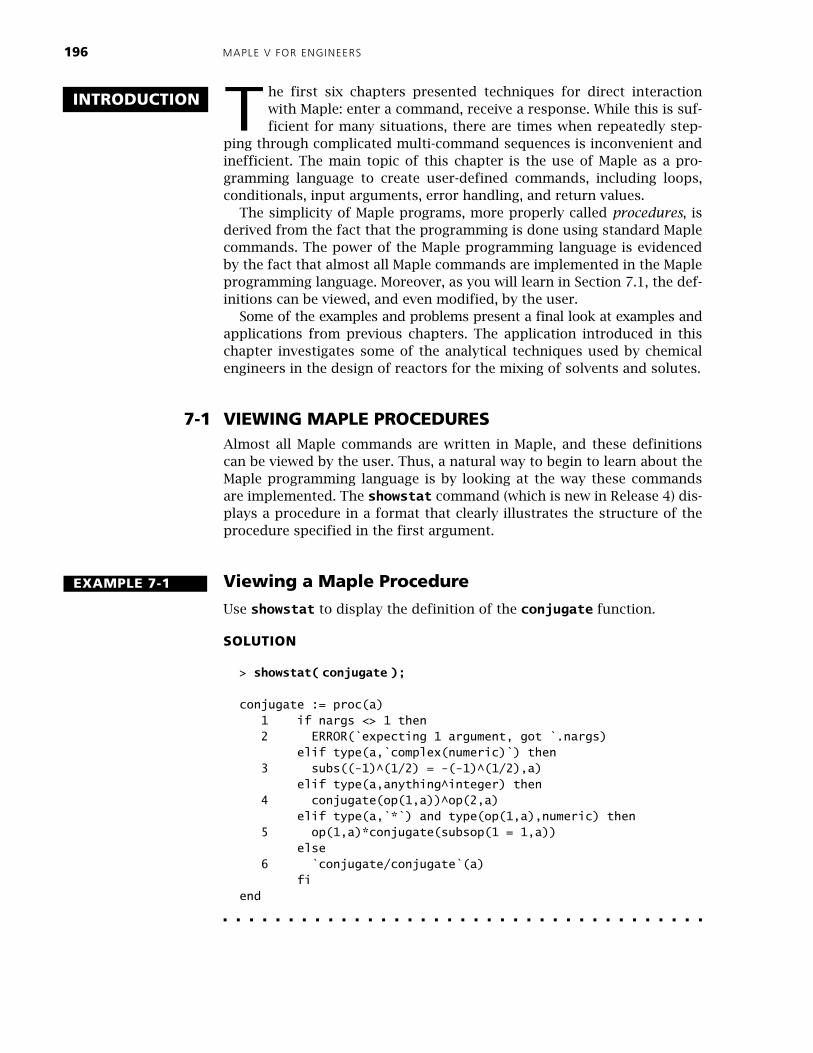
Viewing a Maple Procedure
Use
showstat
to display the definition of the
conjugate
function.
SOLUTION
>
showstat(
conjugate
);
conjugate := proc(a) 1 if nargs <> 1 then 2 ERROR(`expecting 1 argument, got `.nargs) elif type(a,`complex(numeric)`) then 3 subs((-1)^(1/2) = -(-1)^(1/2),a) elif type(a,anything^integer) then 4 conjugate(op(1,a))^op(2,a) elif type(a,`*`) and type(op(1,a),numeric) then 5 op(1,a)*conjugate(subsop(1 = 1,a)) else 6 `conjugate/conjugate`(a) fi
end
TINTRODUCTION
EXAMPLE 7-1
CHAPTER 7 INTRODUCTION TO MAPLE PROGRAMMING
197
Note that the first unnumbered line of the definition says that
conjugate
is defined to be a
procedure
(
proc
...
end
) with one formal argument (
a
).The body of the procedure, the lines numbered 1 through 6, illustratesMaple’s
conditional statement
(
if
...
then
...
elif
...
else
...
fi
). The
end
indi-cates the end of the procedure’s body. The value returned by
conjugate
is the value of the last command executed in the procedure.The conditional statement is not difficult to understand. The Boolean
expression in line 1 checks the arguments for errors. If
conjugate
iscalled with more than one argument, or no arguments, then
nargs<>1
willevaluate to
true
, execution of
conjugate
will terminate, and an errormessage will be generated. If there is exactly one argument, then process-ing continues by checking the Boolean expressions in the
elif
lines. If allof the Boolean expressions evaluate to
false
, then the commandfollowing the
else
is executed.
Determine input arguments that will be processed by each of the five dif-
ferent cases in the definition of
conjugate
.
Since a procedure is a Maple object, the
print
command provides a secondmethod for viewing the definition of a command. One complication withthe use of
print
is that, by default, Maple does not display the body of proce-dures. To override this default, the command
interface(
verboseproc=2):
should be executed. (The
eval
command produces the same outputas
print
.)
Another Method for Viewing a Maple Procedure
Use
print
to display the definition of
conjugate
. How does this comparewith the display produced by
showstat
?
SOLUTION
Before the interface default is changed, printing a procedure simplyshows that
conjugate
is a procedure with one formal parameter.
>
print(
conjugate
);
proc
(
a
) ... end
When the printing of procedure bodies is enabled, the result is
>
interface(
verboseproc=2
):
>
print(
conjugate
);
proc
(
a
)
option `Copyright (c) 1995 by Waterloo Maple Inc. All rights reserved.`;if nargs ≠ 1 then ERROR (`expecting 1 argument, got `.nargs)elif type (a, `complex(numeric)`) then subs(I=-I,a)elif type (a, anything^integer) then conjugate(op(1,a))^op(2,a)elif type (a, `*`) and type(op(1,a), numeric) thenop(1,a)*conjugate(subsop(1=1,a))
else `conjugate/conjugate`(a)fi
end
Try It
!
EXAMPLE 7-2
198 MAPLE V FOR ENGINEERS
Differences between the output produced by print and by showstatinclude the inclusion of line numbers by showstat and the use of differ-ent fonts and styles to distinguish names, functions, and reserved wordsby print. Note also that I is displayed by print, but showstat uses the
internal representation ((-1)^(1/2)).
For short procedures, the differences between print and showstat areoften a matter of personal taste. For longer procedures, however, the abil-ity to display selected lines from a procedure with showstat can beextremely useful. The line numbers correspond to the line numbers pro-duced by showstat and are specified in the optional second argument asa single number or as a range.
Viewing a Portion of a Procedure
Display the first three lines of the definition of conjugate.
SOLUTION
> showstat( conjugate, 1..3 );
conjugate := proc(a) 1 if nargs <> 1 then 2 ERROR(`expecting 1 argument, got `.nargs) elif type(a,'complex(numeric)') then 3 subs((-1)^(1/2) = -(-1)^(1/2),a) elif type(a,anything^integer) then ... elif type(a,`*`) and type(op(1,a),numeric) then ... else ... fiend
The proc and end lines are always displayed by showstat. The condi-tional command (line 1) includes the elif, else, and fi lines even though
they do not appear within the specified lines in the definition.
The definition of the dsolve command is quite long (93 numbered lines). The first few lines check the input arguments, then a conditional is used to determine the method to use to attempt to solve the equation. Use showstat to a) display the part of dsolve that looks for errors in the arguments and b) display the conditional statement that shows the tests Maple applies to determine the algorithm to use to attempt to solve the equation.
EXAMPLE 7-3
Try It
!
CHAPTER 7 INTRODUCTION TO MAPLE PROGRAMMING 199
The only commands that cannot be displayed using showstat, print, oreval are the built-in commands. These are typically the most fundamentalcommands and other commands whose Maple implementation would benoticeably inefficient. Examples of built-in commands include subs, op,sort, and diff.
7-2 FUNCTIONAL OPERATORSAs the examples in Section 7.1 illustrate, the proc ... end command isthe primary Maple command used to define a Maple procedure. The arrowoperator (->), which you first encountered in Chapter 3, can be used todefine simple procedures, called functional operators, which consist of asingle command. In general, while the arrow operator is somewhat sim-pler to use than proc ... end, its main use is for implementing mathe-matical functions, for example, f := (x,y) -> (x^2-y^2)/(x^2+y^2);.
Example 3-8 Revisited with Functional Operators
In Example 3-8 you created the sorted list of integers, through 1 million,that are both perfect squares and cubes. Use the arrow operator and themember command to define a procedure, checkSC, whose input argumentis a single integer, n, and returns true if n is both a perfect square andcube and false in all other cases.
SOLUTION
From the solution to Example 3-8, the following commands create thesorted list of perfect squares and cubes that do not exceed 1 million.
The simplest Maple procedure that meets the requirements of thisproblem is
> checkSC := n -> member( n, SClist );
checkSC := n -> member(n, SClist)
To test this procedure, call checkSC for a variety of input arguments.
> checkSC( 64 );
true
> checkSC( 65 );
false
EXAMPLE 7-4
200 MAPLE V FOR ENGINEERS
The implementation of checkSC in Example 7-4 assumes that the argu-ment is a single number. One means of overcoming this limitation is themap command, which applies a procedure, specified as its first argument,to each operand of the expression specified in the second argument. If theprocedure requires additional arguments, these can be specified asoptional arguments to map.
Determine, in a single statement, which powers of 2 are in SClist. (Hint: Use $ to create the list of all powers of 2 that do not exceed 1 million.)
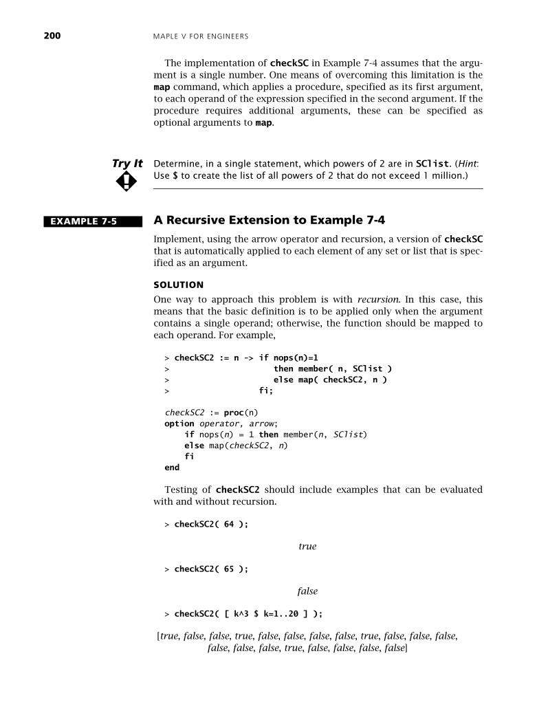
A Recursive Extension to Example 7-4
Implement, using the arrow operator and recursion, a version of checkSCthat is automatically applied to each element of any set or list that is spec-ified as an argument.
SOLUTION
One way to approach this problem is with recursion. In this case, thismeans that the basic definition is to be applied only when the argumentcontains a single operand; otherwise, the function should be mapped toeach operand. For example,
> checkSC2 := n -> if nops(n)=1> then member( n, SClist )> else map( checkSC2, n )> fi;
checkSC2 := proc(n)option operator, arrow; if nops(n) = 1 then member(n, SClist) else map(checkSC2, n) fiend
Testing of checkSC2 should include examples that can be evaluatedwith and without recursion.
It might seem that the simpler definitioncheckSC3 := n -> map(member,n,SClist); fulfills the requirements of Example 7-5, without resorting to recursion. Show that checkSC2 and checkSC3 are not equivalent by finding one argument for which different results are obtained.
Recursion can be very useful, but it should not be overused. In particular,one of the quickest ways to kill a Maple session is to define a recursivefunction whose stopping state is never satisfied. (See the Maple V Pro-gramming Guide, Section 1.2, for additional comments on the use ofrecursion in Maple.)
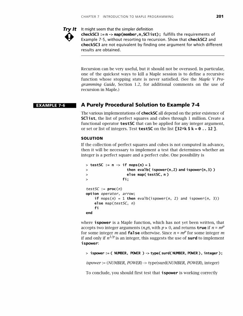
A Purely Procedural Solution to Example 7-4
The various implementations of checkSC all depend on the prior existence ofSClist, the list of perfect squares and cubes through 1 million. Create afunctional operator testSC that can be applied for any integer argument,or set or list of integers. Test testSC on the list [32^k $ k = 0 .. 12 ].
SOLUTION
If the collection of perfect squares and cubes is not computed in advance,then it will be necessary to implement a test that determines whether aninteger is a perfect square and a perfect cube. One possibility is
> testSC := n -> if nops(n) = 1> then evalb( ispower(n,2) and ispower(n,3) )> else map( testSC, n )> fi;
testSC := proc(n)option operator, arrow; if nops(n) = 1 then evalb(ispower(n, 2) and ispower(n, 3)) else map(testSC, n) fiend
where ispower is a Maple function, which has not yet been written, thataccepts two integer arguments (n,p), with p > 0, and returns true if n = mp
for some integer m and false otherwise. Since n = mp for some integer mif and only if n1/p is an integer, this suggests the use of surd to implementispower:
> ispower := ( NUMBER, POWER ) -> type( surd( NUMBER, POWER ), integer );
Thus, from this list of 13 integers, only 3 are perfect squares and cubes.
Compare the results obtained in Example 7-6 with those obtained by applying the appropriate version of checkSC to pow32.
The specific integers from pow32 that are perfect squares and cubes canbe found by careful counting. The select command provides a more gen-eral method of selecting elements of a list, set, sum, product, or functionthat meet a prescribed Boolean condition. The remove command is simi-lar, except that the output is formed by removing all elements that meetthe condition. For example, to extract the five entries from pow32 that areperfect cubes
Use select and testSC to identify the three elements of pow32 that were identified as perfect squares and cubes in Example 7-6.
Try It
!
Try It
!
CHAPTER 7 INTRODUCTION TO MAPLE PROGRAMMING 203
The map command, and its close relative map2, can be used for functionswith more than one argument. For example, map( ispower, pow32, 3 );checks if each element of the pow32 is an integer power of 3. Similarly,map2( ispower, 64, [ 2, 3, 4 ] ); determines if 64 is a perfect square,cube, or quartic power. Note that, for both map and map2, only one argu-ment of the function changes and the difference between map and map2 isthe location of the argument that changes.
7-3 TYPE CHECKING, ERROR, AND RETURNThe testSC procedure defined in Example 7-6 is written with the implicitassumption that the argument is an integer or a compound object whoseoperands are integers.
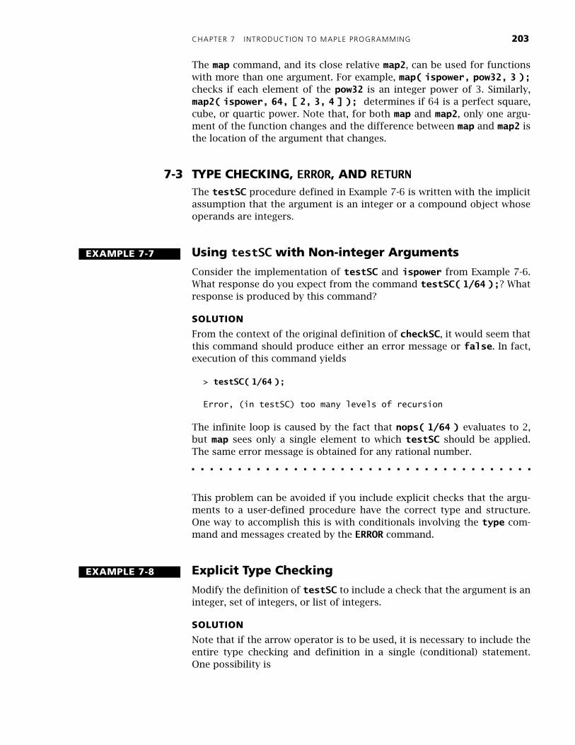
Using testSC with Non-integer Arguments
Consider the implementation of testSC and ispower from Example 7-6.What response do you expect from the command testSC( 1/64 );? Whatresponse is produced by this command?
SOLUTION
From the context of the original definition of checkSC, it would seem thatthis command should produce either an error message or false. In fact,execution of this command yields
> testSC( 1/64 );
Error, (in testSC) too many levels of recursion
The infinite loop is caused by the fact that nops( 1/64 ) evaluates to 2,but map sees only a single element to which testSC should be applied.
The same error message is obtained for any rational number.
This problem can be avoided if you include explicit checks that the argu-ments to a user-defined procedure have the correct type and structure.One way to accomplish this is with conditionals involving the type com-mand and messages created by the ERROR command.
Explicit Type Checking
Modify the definition of testSC to include a check that the argument is aninteger, set of integers, or list of integers.
SOLUTION
Note that if the arrow operator is to be used, it is necessary to include theentire type checking and definition in a single (conditional) statement.One possibility is
EXAMPLE 7-7
EXAMPLE 7-8
204 MAPLE V FOR ENGINEERS
> testSC := n ->> if not type(n,integer,set(integer),list(integer)) then> ERROR(`argument must be an integer or a list or set of integers`)> elif nops(n)=1 then> evalb( ispower(n,2) and ispower(n,3) )> else> map( testSC, n )> fi;
testSC := proc(n)option operator, arrow;if not type(n, list(integer), set(integer), integer) thenERROR(`argument must be an integer or a list or set of integers`)
elif nops(n) = 1 then evalb(ispower(n, 2) and ispower(n, 3))else map(testSC, n)fi
end
Note that normal usage has not been changed
> testSC( 64 );
true
> testSC( [ 1, -1, 64 ] );
[true, false, true]
while noninteger data is now reported as invalid
> testSC( 1/64 );
Error, (in testSC) argument must be an integer or a list or set of integers
> testSC( [ 1, 2, 1/6 ] );
Error, (in testSC) argument must be an integer or a list or set of integers
Observe that even though the arrow operator is used to define checkSC2and testSC, the printed version that appears immediately after the defini-tion uses the proc ... end structure. The only indication that these proce-
dures came from an arrow operator is the line ( option operator, arrow; ).
Maple’s type-based pattern matching provides a second technique tocheck that input arguments are of a specific type. To use this feature forchecking arguments of a procedure, simply append the string :: and theappropriate type specification immediately following the appropriatename in the argument list, for example n :: integer. In particular, x :: tis a synonym for type( x, t ). Additional information about patternmatching can be found under the help topic typematch. For informationabout the description of types, see the type, type,surface, andtype,structure help worksheets.
CHAPTER 7 INTRODUCTION TO MAPLE PROGRAMMING 205
Automatic Pattern Matching
Rewrite the version of testSC in Example 7-8 in a form that uses Maple’stype-based pattern matching. Compare the output from this procedureand the one in Example 7-8.
SOLUTION
The only modification that is required is to move the description of a validargument from the first part of the conditional to the left-hand side of thearrow operator, which must be enclosed in parentheses.
> testSC := ( n :: integer,set(integer),list(integer) ) ->> if nops(n)=1 then> evalb( ispower(n,2) and ispower(n,3) )> else> map( testSC, n )> fi;
testSC := proc(n::list(integer), set(integer), integer)option operator, arrow; if nops(n) = 1 then evalb(ispower(n, 2) and ispower(n, 3)) else map(testSC, n) fiend
The tests of this implementation show its equivalence to the implemen-tation in Example 7-8:
> testSC( 64 );
true
> testSC( [ 1, -1, 64 ] );
[true, false, true]
> testSC( 1/64 );
Error, testSC expects its 1st argument, n, to be of type list(integer), set(integer), integer, but received 1/64
> testSC( [ 1, 2, 1/6 ] );
Error, testSC expects its 1st argument, n, to be of type list(integer), set(integer), integer, but received [1, 2, 1/6]
The only difference between the implementations in Example 7-8 andthis one is that the error messages created with the automatic patternmatching are more informative than the simple messages generrated in
Example 7-8.
EXAMPLE 7-9
206 MAPLE V FOR ENGINEERS
Rewrite the ispower procedure so that it generates error messages when the first argument is not an integer and the second argument is not a pos-itive integer. (Select appropriate test cases that test all aspects of the new definition.)
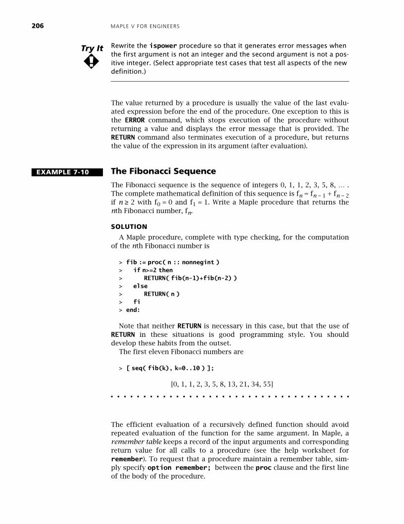
The value returned by a procedure is usually the value of the last evalu-ated expression before the end of the procedure. One exception to this isthe ERROR command, which stops execution of the procedure withoutreturning a value and displays the error message that is provided. TheRETURN command also terminates execution of a procedure, but returnsthe value of the expression in its argument (after evaluation).
The Fibonacci Sequence
The Fibonacci sequence is the sequence of integers 0, 1, 1, 2, 3, 5, 8, … .The complete mathematical definition of this sequence is fn = fn − 1 + fn − 2if n ≥ 2 with f0 = 0 and f1 = 1. Write a Maple procedure that returns thenth Fibonacci number, fn.
SOLUTION
A Maple procedure, complete with type checking, for the computationof the nth Fibonacci number is
> fib := proc( n :: nonnegint )> if n>=2 then> RETURN( fib(n-1)+fib(n-2) )> else> RETURN( n )> fi> end:
Note that neither RETURN is necessary in this case, but that the use ofRETURN in these situations is good programming style. You shoulddevelop these habits from the outset.
The first eleven Fibonacci numbers are
> [ seq( fib(k), k=0..10 ) ];
[0, 1, 1, 2, 3, 5, 8, 13, 21, 34, 55]
The efficient evaluation of a recursively defined function should avoidrepeated evaluation of the function for the same argument. In Maple, aremember table keeps a record of the input arguments and correspondingreturn value for all calls to a procedure (see the help worksheet forremember). To request that a procedure maintain a remember table, sim-ply specify option remember; between the proc clause and the first lineof the body of the procedure.
Try It
!
EXAMPLE 7-10
CHAPTER 7 INTRODUCTION TO MAPLE PROGRAMMING 207
Creating a Remember Table
Modify the definition of fib in Example 7-10 to create a new procedure,Fib, that uses a remember table.
SOLUTION
The only modifications are the renaming of the procedure and theinsertion of option remember; immediately following the proc command.
> Fib := proc( n :: nonnegint )> option remember;> if n>=2 then> RETURN( Fib(n-1)+Fib(n-2) )> else> RETURN( n )> fi> end:
A simple test that this function works as expected is:
> Fib( 10 );
55
The number of function calls, cn, required to compute fn without the use of a remember table can be shown to satisfy the recurrence relationcn = cn − 1 + cn − 2 + 1 for n ≥ 2 with c0 = 1 and c1 = 1. Write a Maple proce-dure that efficiently computes cn.
7-4 REPETITION LOOPSMost modern programming languages provide some form of loop controlstructure. In Maple the repetition statement is the for ... while ...do ... od command. Any combination of the for and while clauses canbe specified; only the do and od are required.
Using Repetition to Sum a Collection of Numbers
Use the repetition statement to find the sum of the squares of the firstten Fibonacci numbers.
EXAMPLE 7-11
Try It
!
EXAMPLE 7-12
208 MAPLE V FOR ENGINEERS
SOLUTION
> SUM := 0; for N from 1 to 10 by 1 do SUM := SUM + Fib(N) od;
SUM := 0
SUM := 1
SUM := 2
SUM := 4
SUM := 7
SUM := 12
SUM := 20
SUM := 33
SUM := 54
SUM := 88
SUM := 143
The syntax of the repetition statement is fairly straightforward. The namefollowing for identifies the loop index; the from clause sets the initialvalue for the loop index (if omitted, the initial value is 1); the by clausesets the step for each iteration (if omitted, this is also assumed to be 1);the to clause identifies the final value of the loop index. If the to is omit-ted, the loop will generally be terminated via a break statement inside therepetition loop or a while clause. The while clause specifies a Booleancondition that is checked at the beginning of each loop (the loop contin-ues as long as this expression evaluates to true). The do and od denotethe beginning and end of the sequence of expressions that are executedduring each pass through the loop. For a full description of this commandplease see the help worksheet for do.
Another Sum Using Repetition
Use the repetition statement to compute the sum of the square of the first10 prime numbers.
SOLUTION
A straightforward solution is to start with the smallest prime and add thesquare of each prime until ten primes have been found. As a cross-check,keep a list of the primes as they are encountered.
EXAMPLE 7-13
CHAPTER 7 INTRODUCTION TO MAPLE PROGRAMMING
209
To implement this plan it is necessary to keep track of the number ofprimes that have been found, the list of primes, and the sum of thesquares of the primes:
>
COUNT
:=
0;
PRIMES
:=
NULL;
SUM
:=
0;
COUNT
:= 0
PRIMES
:=
SUM
:= 0
The remainder of the algorithm is represented by
>
for
N
from
2
by
1
while
COUNT<10
do
>
if
isprime(N)
then
>
COUNT:=COUNT+1;
>
PRIMES:=PRIMES,N;
>
SUM:=SUM+N^2;
>
fi
>
od;
In this case, the results of executing this loop are
>
COUNT;
PRIMES;
SUM;
10
2, 3, 5, 7, 11, 13, 17, 19, 23, 29
2397
Moreover, the loop index retains its final value
>
N;
30
Another way to approach Example 7-13 is to use a loop to determine the appropriate collection of primes as a list or set, then use other methods to compute the square of each prime and to find the sum of the squares. Write a Maple procedure,
sumprime
, that computes the sum of the
squares of the next
n
primes greater than or equal to
p
. Both
n
and
p
will normally be specified as arguments; if only one argument is provided,
assume it is
p
and that
n
=
1.
Try It
!
210 MAPLE V FOR ENGINEERS
A second variation of the repetition statement is designed for use when thevalues for the index variable are to be taken from a list or set, not a geo-metric progression. The syntax for this is the same, except that for ...in ... replaces for ... from ... to ... by ... .
Using Repetition in a Sum
Write a Maple procedure, minpos, that uses the repetition statement tofind the smallest positive number from a list or set of numbers. (Be sureto include type checking.) An alternate implementation of minpos is dis-cussed in Problem 4 at the end of this chapter.
Use Maple’s random number generator, rand, to generate test data forminpos.
SOLUTION
The only real issue here is how to initialize the counter used to keep trackof the smallest positive number. Two possibilities are to initialize thecounter to the largest element in the set (MIN := max(DATA)) or to NULL(the empty expression). Using the latter of these options, the procedurecan be written as
> minpos := proc( DATA :: set(constant), list(constant) )> MIN := NULL;> for N in DATA do> if N > 0 then MIN := min( MIN, N ) fi;> od;> RETURN( MIN );> end:
Warning, `MIN` is implicitly declared localWarning, `N` is implicitly declared local
The help worksheet for rand indicates that a random number genera-tor, RNG, with integer values in the interval [ −100, 100 ] is created with thecommand
7-5 LOCAL AND GLOBAL VARIABLESThe definition of minpos in Example 7-14 produced a warning messageabout a variable being “implicitly declared local.” Each variable appearingin a Maple procedure is either a local, global, or environment variable.Local variables are known only within this call to the procedure and areindependent of any other use of this name. Environment variables are aspecial type of global variable (see the help worksheet for the topic envvar).
Global variables should be used only when they are absolutely neces-sary. In situations that justify the use of a global variable, the names ofeach global variable should be chosen to be descriptive and prevent inad-vertant modification by any other Maple procedure. Short names shouldbe avoided unless they are preceded by a special character such as anunderscore. While Maple has specific rules for deciding if a variable islocal or global by default (see the help worksheet for procedure), it is goodprogramming technique to explicitly declare all local and global variables.
Consider the following procedure:
> newname := proc()> global _N;> if not(assigned( _N )) then _N:=0 fi;> for _N from _N+1 while assigned( C._N ) do od;> RETURN( C._N )> end:> _N := '_N':
There are two new commands in the definition of newname. The assignedcommand is easily understood from the online help worksheet; . is theconcatenation or dot operator (see the help topic dot), which is used hereto append a number to the name C to form new Maple names.
Illustrating the Use of Global Variables
Suppose the following assignments are made:
> C2:=1: C4:=1.2: C5:=a: C8:=C2:
Explain the output produced when the following sequence of com-mands is executed:
The first call to newname assigns _N the value 0, then returns C1 since thisname has not been assigned a value. The value of _N is now 1. The secondtime newname is called, it takes two steps to find an unassigned name.
> newname() * sin(x) + newname() * cos(x);
C1 sin(x) + C3 cos(x)
The current value of _N is 3.
> _N;
3
The third and fourth calls to newname are similar. The final value for _Nshould be 7.
> newname() * exp(x) + newname() * exp(-x);
C6 ex + C7 e(−x)
> _N;
7
7-6 DIGGING DEEPER AND DEBUGGINGA complete description of Maple’s debugging system cannot be providedwithin the scope of this module. The commands most commonly used dur-ing the development of Maple procedures are debug, trace, printlevel,and maplemint. The debug and trace commands can be used to see theresults of each command that is executed in a procedure; once enabled, thisfeature is disabled with undebug or untrace (see the help worksheets fordebug). Each command is associated with a level. By default, the results ofall commands at level 1 are displayed; the results of commands at higherlevels can be displayed by increasing the value assigned to printlevel(see the help worksheet for printlvl). The syntax checker, maplemint,detects syntax errors and identifies potential problems with local and glo-bal variables (see the online help for maplemint).
The Maple debugger is another tool which can be useful when program-ming with Maple. With the debugger you can specify breakpoints and watch-points within a procedure. A breakpoint is a line number, as reported byshowstat, where execution of the procedure pauses; a watchpoint interrupts
CHAPTER 7 INTRODUCTION TO MAPLE PROGRAMMING
213
execution of the procedure whenever a specified variable is assigned avalue or an error occurs. For specific information on the use of the Mapledebugger, or any of the other programming tools mentioned in this sec-tion, consult the online help topics
debugger
and
debug
.
SOLVENTS AND SOLUTES
Chemical engineers frequently combine different substances in reactorsand employ reactor models to synthesize and analyze a variety of prod-ucts ranging from drugs to synthetic materials. This application willshow how the principle of conservation of mass can be used to developa model for a simple reactor in which a solute is combined with a sol-vent to produce a new solution. The model, which leads to a differentialequation, will be analyzed graphically and qualitatively without explic-itly finding a solution. The two quantities of particular interest in thisanalysis are the concentration and mass of solvent in the reactor at anytime while the reactor is in operation. The amount of usable solutionthat is produced by this reactor and other issues are discussed in Prob-lems 10–14 at the end of this chapter.
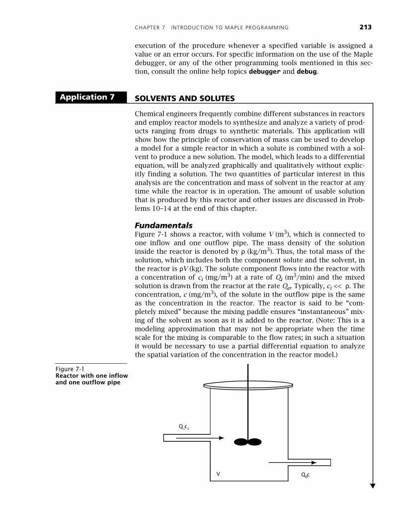
Fundamentals
Figure 7-1 shows a reactor, with volume
V
(m
3
), which is connected toone inflow and one outflow pipe. The mass density of the solutioninside the reactor is denoted by
ρ
(kg/m
3
). Thus, the total mass of thesolution, which includes both the component solute and the solvent, inthe reactor is
ρ
V
(kg). The solute component flows into the reactor witha concentration of
c
i
(mg/m
3
) at a rate of
Q
i
(m
3
/min) and the mixedsolution is drawn from the reactor at the rate
Q
o
. Typically,
c
i
<<
ρ
. Theconcentration,
c
(mg/m
3
), of the solute in the outflow pipe is the sameas the concentration in the reactor. The reactor is said to be “com-pletely mixed” because the mixing paddle ensures “instantaneous” mix-ing of the solvent as soon as it is added to the reactor. (Note: This is amodeling approximation that may not be appropriate when the timescale for the mixing is comparable to the flow rates; in such a situationit would be necessary to use a partial differential equation to analyzethe spatial variation of the concentration in the reactor model.)
Application 7
Figure 7-1
Reactor with one inflow and one outflow pipe
V
Q c
Q c
ii
o
214 MAPLE V FOR ENGINEERS
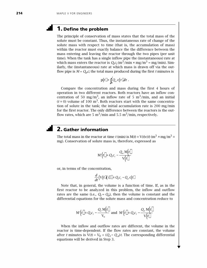
1. Define the problem
The principle of conservation of mass states that the total mass of thesolute must be constant. Thus, the instantaneous rate of change of thesolute mass with respect to time (that is, the accumulation of mass)within the reactor must exactly balance the the difference between themass entering and leaving the reactor through the two pipes (per unittime). When the tank has a single inflow pipe the (instantaneous) rate atwhich mass enters the reactor is Qici (m
3/min × mg/m3 = mg/min). Sim-ilarly, the (instantaneous) rate at which mass is drawn off via the out-flow pipe is M = Qoc; the total mass produced during the first t minutes is
.
Compare the concentration and mass during the first 4 hours ofoperation in two different reactors. Both reactors have an inflow con-centration of 50 mg/m3, an inflow rate of 5 m3/min, and an initial(t = 0) volume of 100 m3. Both reactors start with the same concentra-tion of solute in the tank; the initial accumulation rate is 200 mg/minfor the first reactor. The only difference between the reactors is the out-flow rates, which are 5 m3/min and 5.5 m3/min, respectively.
2. Gather information
The total mass in the reactor at time t (min) is M(t) = V(t)c(t) (m3 × mg/m3 =mg). Conservation of solute mass is, therefore, expressed as
or, in terms of the concentration,
Note that, in general, the volume is a function of time. If, as in thefirst reactor to be analyzed in this problem, the inflow and outflowrates are the same (i.e., Qi = Qo), then the volume is constant and thedifferential equations for the solute mass and concentration reduce to
and
When the inflow and outflow rates are different, the volume in thereactor is time-dependent. If the flow rates are constant, the volumeafter t minutes is V(t) = V0 + (Q i − Q o)t. The corresponding differentialequations will be derived in Step 3.
p ct Q do
t
( ) = ( )∫ τ τ0
′( ) = −( )
( )MM
Vt Q c
Q t
ti i
o
ddt
t t Q c Q ti i oV c c( ) ( )( ) = − ( )
′( ) = −( )
MM
Vt Q c
Q ti i
i
0
′( ) = −( )
( )MM
Vt Q c
Q t
ti i
o
CHAPTER 7 INTRODUCTION TO MAPLE PROGRAMMING 215
The last piece of information needed to complete the mathematicaldescription of the reactor is the initial condition. Since only the initialaccumulation rate is provided, some work is needed to compute the ini-tial concentration or initial mass. In general, if the initial accumulation
rate is A mg/min, that is, (at t = 0), then, using the differen-
tial equation for the mass evaluated at t = 0, . From
here it is not difficult to obtain an expression for the initial mass interms of known quantities; dividing the initial mass by the initial vol-ume yields the initial concentration.
The common parameter values for the two reactors are the initial vol-ume, initial accumulation rate, inflow concentration, and inflow rate:V0 = 100 m3, A = 200 mg/min, Qi = 5 m3/min, and ci = 50 mg/m3. Thefirst reactor has an outflow rate of Qo = 5 m3/min while the drain fromthe second tank flows at a rate of 5.5 m3/min.
3. Generate and evaluate potential solutions
The problem asks for a qualitiative description of the mass and concen-tration during a four hour time period. Since you have two differentreactors to analyze—and might reasonably expect to be asked to ana-lyze more in the future—a good approach is to create a general proce-dure for producing plots of the mass and concentration over a giventime interval.
The procedure, which will be called plotCM, will use DEplot to createplots of the mass and concentration and display to place the plotsside by side. The arguments to DEplot must contain the differentialequation, the name of the dependent variable (either M or c), the rangeof the independent variable (for example, t = 0 .. 240), and the initialcondition; all other arguments are optional. If conservation of mass isencoded directly into plotCM, the arguments to plotCM will need tosupply the volume (as a function of time), values for all other parame-ters, and the time interval on which the solutions should be plotted.This suggests that plotCM can be divided into three steps: verificationof the arguments, derivation of the differential equations and initialconditions, and creation and display of the plots.
The middle step requires the most thought and planning. It can behelpful to interactively test the individual steps involved in the derivationof the initial value problems. To see exactly how each differential equa-tion and initial condition can be obtained from conservation of mass,recall that the principle of conservation of mass can be expressed as
The specific differential equation for the mass of solute in a reactor isobtained by specifying the volume and values for all other parameters.
> odeM := ConsMass;
The corresponding differential equation for the concentration can beobtained by using the identity M(t) = c(t)V(t) in the conservation of massequation and forcing evaluation of the expression, and then solving forthe rate of change of the concentration:
Recall that the two reactors have different outflow rates but have thesame initial conditions. Since all other parameters are the same, the initialaccumulation rate must be different for the two reactors. In the currentcontext, it is easier to compute the initial mass and pass this value,along with the values for
c
i
,
Q
i
, and
Q
o
, to
plotCM
. For this reason itseems prudent to implement the initial conditions as
>
icM
:=
M(0)
=
M[0];
>
icC
:=
c(0)
=
M[0]/V(0);
Now that the specific set of parameters has been identified and analgorithm for determining the initial value problems has been tested, itis time to combine everything and write the
plotCM
procedure.
>
plotCM
:=
proc(PARAM
::
set(
name=realcons
)
,
>
VOLUME
::
identical(V)=realcons,dependent(t),
>
TRANGE
::
identical(t)=range(realcons)
)
>
local
odeM,
odeC,
icM,
icC,
ConsMass,
_pM,
_pC,
NAMES,
OPTS;
>
NAMES
:=
map(lhs,op(PARAM));
>
#
check
that
all
parameters
are
specified
>
if
evalb(
NAMES
<>
c[i],Q[i],Q[o],M[0]
)
then
>
ERROR(`must
specify
c[i],
Q[i],
Q[o]
and
M[0]`)> fi;> # default DEplot options> OPTS := arrows=NONE, linecolor=BLUE, stepsize=1;> # user-specified DEplot options> if nargs>3 then OPTS := OPTS, args[4..nargs] fi;> # assemble initial value problems from conservation of mass> ConsMass := diff( M(t), t ) = Q[i] * c[i] - Q[o] * M(t) / V ;> odeM := subs( VOLUME, PARAM, ConsMass );> odeC := value( subs( M(t)=c(t)*V, VOLUME, PARAM, ConsMass ) );> odeC := op( solve( odeC, diff( c(t), t ) ) );> icM := subs( PARAM, M(0) = M[0] );> icC := subs( VOLUME, PARAM, t=0, c(0) = M[0]/V );> # create separate plots, then display side by side> _pM := DEtools[DEplot]( odeM, M, TRANGE, [[icM]],> title=`M (mg) vs. t (min)`, OPTS );> _pC := DEtools[DEplot]( odeC, c, TRANGE, [[icC]],> title=`c (mg/m^3) vs. t (min)`, OPTS );> plots[display]( array( [_pM,_pC] ) );> end:
Text that comes after a # is ignored by Maple. These comments,which are not displayed when the procedure is viewed by print orshowstat, are included as aids for anyone who wants to understandplotCM, now or in the future. Note that, in addition to processing thethree required arguments, this implementation of plotCM uses nargs,the number of arguments in the current procedure call, and args, thelist of arguments for the current procedure call, to forward anyoptional arguments to the DEplot commands. The only other specialfeature of this procedure is the explicit reference to the libraries to
icM M
icCM
: M
: cV
= ( ) =
= ( ) = ( )
0
00
0
0
218 MAPLE V FOR ENGINEERS
which DEplot and display belong; this is done to ensure that plotCMworks even when the complete DEtools and plots packages have notbeen loaded in the current session.
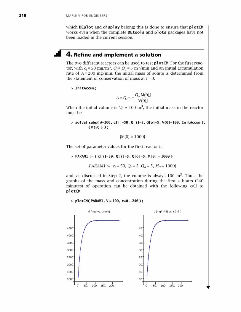
4. Refine and implement a solution
The two different reactors can be used to test plotCM. For the first reac-tor, with ci = 50 mg/m3, Qi = Qo = 5 m3/min and an initial accumulationrate of A = 200 mg/min, the initial mass of solute is determined fromthe statement of conservation of mass at t = 0:
> InitAccum;
When the initial volume is V0 = 100 m3, the initial mass in the reactormust be
and, as discussed in Step 2, the volume is always 100 m3. Thus, thegraphs of the mass and concentration during the first 4 hours (240minutes) of operation can be obtained with the following call toplotCM:
> plotCM( PARAM1, V = 100, t=0..240 );
A Q cQ
i io= − ( )
( )M
V
0
0
c (mg/m^3) vs. t (min)M (mg) vs. t (min)
45.
40.
35.
30.
25.
20.
15.
10.
200.150.100.50.0
4500.
4000.
3500.
3000.
2500.
2000.
1500.
1000.
200.150.100.50.0
CHAPTER 7 INTRODUCTION TO MAPLE PROGRAMMING 219
Note that, except for the scales, these curves appear to have the samequalitative behavior. From their initial values, both the mass and con-centration increase rapidly to a constant level. The concentrationclearly approaches 50 mg/m3, which is the value of ci. Do you under-stand why this must be the case? The mass approaches 100 times thisvalue, that is, 5 g.
The plots produced by plotCM are useful for understanding thebehavior of the solution to this one problem. One means of determiningif this behavior changes with different initial conditions is to includethe direction fields for each differential equation in the plot. Directionfields are produced by DEplot when, for example, the arrows=SMALLoptional argument is specified. Since plotCM automatically forwardsoptional arguments to DEplot, it suffices to include this optional argu-ment after the three required arguments for plotCM. In the case of thisfirst reactor, you should see that all solutions with initial concentrationsbelow 50 mg/m3 have the same qualitative behavior. (See Problem 14 atthe end of this chapter.)
The second reactor differs only in the output flow rate
Because the input and output flow rates are not equal, the volumeis not constant. In this case the volume in the reactor decreases by1/2 cubic meter per minute. The request for graphs of the mass andconcentration during the first 4 hours of operation is made with thesingle command:
> plotCM( PARAM2, V=100-t/2, t=0..240 );
Error, (in DEtools/DEplot/drawlines) Stopping integration due to, division by zero
The error message indicates that DEplot has encountered division byzero, but does not tell you exactly when or where this occurs. Toexplain and, if possible, provide a resolution to this problem, recall(from Step 3) that both differential equations include the volume in thedenominator of a rational expression:
Since the volume decreases by 1/2 m3/min, the tank is completelyempty after 200 minutes. Thus, the best that can be hoped for is to plotthe solution curves for any time ending before 200 minutes. For exam-ple, the solutions (and direction fields) that terminate one minutebefore the singularity is encountered are:
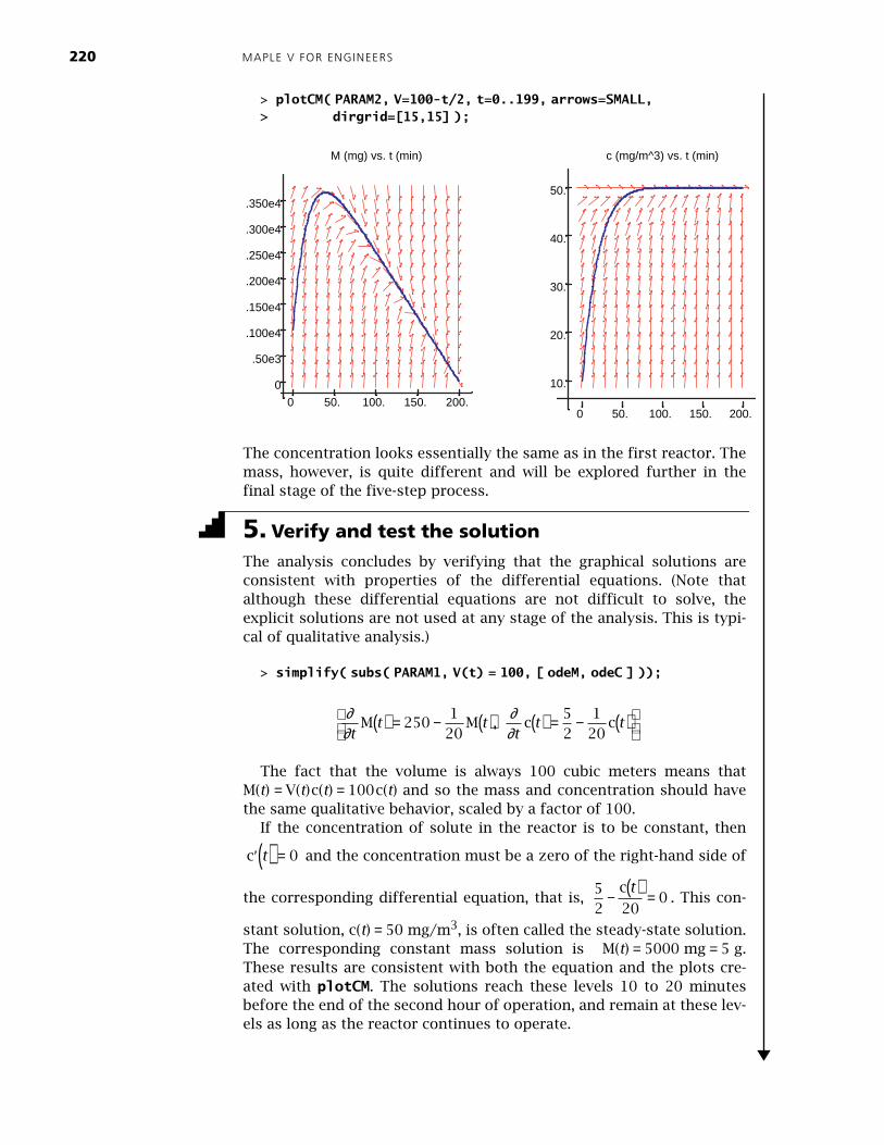
The concentration looks essentially the same as in the first reactor. Themass, however, is quite different and will be explored further in thefinal stage of the five-step process.
5. Verify and test the solution
The analysis concludes by verifying that the graphical solutions areconsistent with properties of the differential equations. (Note thatalthough these differential equations are not difficult to solve, theexplicit solutions are not used at any stage of the analysis. This is typi-cal of qualitative analysis.)
The fact that the volume is always 100 cubic meters means thatM(t) = V(t)c(t) = 100c(t) and so the mass and concentration should havethe same qualitative behavior, scaled by a factor of 100.
If the concentration of solute in the reactor is to be constant, then
and the concentration must be a zero of the right-hand side of
the corresponding differential equation, that is, . This con-
stant solution, c(t) = 50 mg/m3, is often called the steady-state solution.The corresponding constant mass solution is M(t) = 5000 mg = 5 g.These results are consistent with both the equation and the plots cre-ated with plotCM. The solutions reach these levels 10 to 20 minutesbefore the end of the second hour of operation, and remain at these lev-els as long as the reactor continues to operate.
c (mg/m^3) vs. t (min)
50.
40.
30.
20.
10.
200.150.100.50.0
.350e4
.300e4
.250e4
.200e4
.150e4
.100e4
.50e3
0
200.150.100.50.0
M (mg) vs. t (min)
∂∂
∂∂t
t tt
t tM M , c c( ) = − ( ) ( ) = − ( )
2501
2052
120
′( ) =c t 0
52 20
0− ( ) =c t
CHAPTER 7 INTRODUCTION TO MAPLE PROGRAMMING 221
The analysis is somewhat different for the reactor with differentinflow and outflow rates.
While the steady-state concentration is still c(t) = 50 mg/m3, there areno constant solutions to the mass equation. Since the outflow rateexceeds the inflow rate by 1/2 m3/min, it is not surprising that thereactor eventually becomes dry—this is the source of the singularityafter 200 minutes. At this time the reactor ceases to function. Thisproblem is not numerical; it is intimately connected with the specificdesign of this reactor.
In some situations it is necessary to control the concentration and/oramount of solute in the reactor. For example, if the solute is toxic, Occu-pational Safety and Health Administration (OSHA) standards may requirethe manufacturer to keep the concentration under 40 mg/m3. At the sametime, production guidelines may stipulate that the solution is usable onlywhen the concentration exceeds 15 mg/m3. Propose and critique a planfor adapting the reactor to maintain a constant volume and to satisfythese criteria.
One approach would be to start the reactor with the solute entering atits normal rate and concentration. The first few minutes of outflow wouldhave to be discarded or recycled, and then a usable solution would be pro-duced. Just before the concentration reaches the OSHA safety limit, thesource of solute would be interrupted. To maintain a constant volume inthe reactor, the inflow would be pure solution. Just before the concentra-tion of the solution reaches the lower (production) threshold, the solutewould be added to the inflow solution. This process would then repeat forthe remainder of the production run. Try to implement this plan with asequence of calles to plotCM using different parameters and time intervals.
SUMMARY The final topic in this introduction to Maple has been the Maple program-ming language, in particular, the definition of Maple procedures usingboth the arrow operator (->) and proc ... end. The discussion includedissues relating to error handling, return values, type-based pattern matching,and local and global variables. The conditional (if ... then ... else ... fi) andrepetition (for ... while ... do ... od) statements were used in a number ofexamples. Other commands discussed included showstat, select, remove,map, map2, interface, printlevel, debug, and maplemint. The applica-tion utilized the principle of conservation of mass to analyze a mixingproblem, as a chemical engineer might do.
∂∂
∂∂t
tt t
t tt
t
tM
M, c
c( ) =− + + ( )
− +( ) = ( ) −
− +
50000 250 11
20010
50
200
What If
?
222
MAPLE V FOR ENGINEERS
Key Words
Maple Commands
References
1. Chapra, S.C. and Canale, R.P.,
Introduction to Computing for Engineers
, 2nd Ed.,New York: McGraw-Hill, 1994, pp. 664–672.
2. Lindeburg, M.R.,
Engineer-In-Training Reference Manual
, 8th Ed., Belmont, CA:Professional Publications, pp. 10-7 and 10-10.
3. Monagan, M.B., Geddes, K.O., Labahn, G., and Vorkoetter, S.,
Maple V Program-ming Guide
, Springer-Verlag, 1996.4. Nicolaides, R., and Walkington, N.,
Maple programming languageprocedurerandom number generatorrecursionremember tablerepetition statementselection, removaltype-based pattern matchingwatchpoints
->
(arrow operator)
.
(dot or concatenation operator)
::
(type-based pattern matching)
args
,
nargsassigneddebug
,
trace
,
printlevel
,
maplemintERRORfor
...
from
...
to
...
by
...
while
...
do
...
odfor
...
in
...
while
...
do
...
odif
...
then
...
elif
...
else
...
fiinterface
,
verboseproc
isolate
(from
student
package)
local
,
globalmap
,
map2memberNULL
(empty expression)
option
rememberprintproc
...
endrandRETURNselect
,
removeshowstat
CHAPTER 7 INTRODUCTION TO MAPLE PROGRAMMING 223
Concluding Remarks
You have now completed this module of the Engineer’s Toolkit series. Ifyou have worked through the majority of the Examples, Try It!’s, Applica-tions, and Problems in each chapter, you should now have a good under-standing of Maple and some of its uses in engineering. More importantly,you should have the knowledge and confidence to know you can extendyour knowledge to tackle problems that might arise in areas and applica-tions other than those presented here.
Congratulations, and good luck!
Exercises
1. (a) Write a Maple procedure, TIMING, that reports the time needed to evaluate the argument, then returns a list whose first element is the elapsed time and all subsequent elements are the results, if any, of evaluating the argument. The input argument will need to be specified in single quotes (') to prevent evaluation of the argu-ment before the appropriate time in the body of the procedure. (Note that there are several differences between TIMING and the built-in time command; in fact, TIMING will use time.)
(b) Use TIMING to compare three implementations of a procedure that selects all input arguments that are both a perfect square and a perfect cube. Rank the implementations in terms of efficiency. Does this ranking depend on the size of the numbers or number of elements in the set?
cubes( SET ):> SCselect2 := (SET::set(integer)) -> squares( cubes( SET ) ):> SCselect3 := (SET::set(integer)) -> cubes( squares( SET ) ):
2. Write a Maple procedure, plotD, that plots a function (of one variable) and each of its first two derivatives on separate graphs. In order to make the three plots appear side-by-side, display a 1 × 3 array of plots. Include appropriate titles for each plot.
The following three commands should all produce the expected results
Note that only two arguments are required; additional arguments should be passed directly to the plot commands (see ?args for more information about argument lists).
224 MAPLE V FOR ENGINEERS
3. Consider the function Fib implemented in Example 7-11. The else part of the conditional is executed the first time the function is called with an argument of 1 or 0. The same effect can be achieved by explicitly entering these results into the remember table (via standard assignments). This suggests a third implementation for the Fibonacci numbers:
(a) Verify that FIB correctly computes the Fibonacci numbers.
(b) Which of fib, Fib, and FIB is most efficient? (Use TIMING to com-pute f20.) See the forget help worksheet for information on reset-
ting remember tables.
(c) What happens if the two assignments are moved before the defini-tion of FIB?
4. Write an alternate version of minpos (origanally defined in Example7-14) that does not utilize the repetition command. Use TIMING to compare the efficiency of the two implementations.
5. A shaft-position encoder provides a 3-bit signal indicating the posi-tion of a motor shaft in steps of 45 degrees using the following code:
(a) Write a Maple procedure that produces the appropriate encoder output for a shaft position, or list of shaft positions.
(b) Write separate Maple procedures that correspond to binary encod-ers that are ON, that is, returns the value 1, when i) the shaft is in the second half of its rotation cycle, ii) the motor shaft is not in the first eighth of its cycle and iii) either in the first or third quarter of its cycle.
Each encoder should contain all necessary type and error checking. The rand command can be used to generate a random number gener-ator of integers between 0 and 360. For example, one way to generate data for this problem would be as follows:
6. The Chebyshev polynomials of the first kind, Tn(x), satisfy the recur-
rence relations Tn(x) = 2xTn − 1(x) − Tn − 2(x) for n ≥ 2 with T0(x) = 1 and
T1(x) = x.
(a) Write a recursive definition of the Chebyshev polynomials.
(b) Find Maple’s built-in Chebyshev functions. How are these func-tions implemented?
7. Implement a Maple procedure, bodeampplot, that creates the cor-rected Bode amplitude plot for a frequency response function. Your procedure should reproduce the corrected Bode amplitude plot for the circuit in the Electric Filter application (Chapter 6) with L = 10 H, C = 6 µF, and R = 1 kΩ with the following commands:
8. (a) Fuzzy logic was introduced in problem 8 (Chapter 3). Write a
Maple function, mu, so that mu(A) = µA, where
is the membership function for the element A.
Hint: Use the arrow operator.
(b) Write Maple implementations of the three fuzzy logical operations fuzzyNOT, fuzzyOR, fuzzyAND.
Hint: Use convert,piecewise to simplify the maximum and mini-mum of a collection of functions.
(c) Use the procedures created in (a) and (b) to find the membership functions for A = 10, B = 15, C = A, D = A ∪ B, E = A ∩ B,F = 5, 10, 15, 20 , and G = 5, 15, 20 . Plot each of these member-ship functions.
9. This is a continuation of the Try It! at the end of Section 3.2 and prob-lem 9 of Chapter 3.
Write an analog-to-digital converter, d2a, that accepts an analog signal from a specified range and returns the appropriate digital code as a binary number. The three input arguments to the procedure should be: the analog signal (either a single number or a list of numbers), the range of valid signals, and the number of digital codes to be used to represent the code. All output codes should have the same length.
Be sure that your procedure includes all appropriate error checking. Select, and implement, a reasonable way of handling data that is out-side the range of expected signals. (It is not acceptable for the proce-dure to simply report an error and quit.)
µA xx A
( ) =+ −
11 2( )
226 MAPLE V FOR ENGINEERS
Test this procedure using the following sets of commands:
> analog := rand( 0 .. 5000 ) / 1000: # random numbers between 0 and 50> signal := map( evalf, [ seq(analog(), k=1..100) ] ):> d2a( signal, 0..50, 128 );> > noisy := rand( -100 .. 600 ) / 10: # random numbers between -10 and 60> badsignal := map( evalf, [ seq(noisy(), k=1..10 ) ] ):> d2a( noisy, 0..50, 128 );> d2a( noisy, -10..60, 128 );
10. Modify the plotCM procedure to accept an optional argument specify-ing the specific plots to be included in the output. For example, speci-fying plotlist = [M] would produce only the mass plot and plotlist = [C] only the concentration plot; the default would be equivalent to plotlist = [C,M]. Be sure to include appropriate error checking.
11. As part of the process in manufacturing an eye wash product, aboric acid solute enters a tank filled with purified water at time t = 0 minutes. In practice it is not possible to achieve a constant inflowconcentration. One way to model this is to assume the input concen-tration varies sinusoidally with time. That is, instead of ci being a
constant, use
.
where the average inflow rate is ci = 50 mg/m3, the amplitude of the
inflow variation is ca = 40 mg/m3, and T = 50 min is the period.
(Assume all other parameters are the same as in the reactor with con-stant volume.)
(a) Plot the concentration and total mass of boric acid produced by this tank as a function of time.
(b) Does this reactor approach the original (constant inflow) reactor as ca → 0?
(c) How much boric acid is in the tank after three hours? How much boric acid has been produced during this time period?
12. The analysis of the reactor model conducted in the application focused solely on the concentration levels in the reactor. Another aspect of this problem is the quality and quantity of the solution obtained from the reactor.
(a) Show that the total amount of solution produced during the first
t minutes, , satisfies each of the following
differential equations:
i)
ii)
(Assuming the volume in the reactor is held constant.)
c t c ct
Ti i a( ) = +
sin
2π
p ct Q do
t
( ) = ( )∫ τ τ0
′( ) = ( )p ct Q t0
′′( ) + ′( ) =p ptQV
tQ Q c
Vi o i i
0 0
CHAPTER 7 INTRODUCTION TO MAPLE PROGRAMMING 227
(b) Find appropriate initial conditions for each of the equations in (a).
(c) Once the concentration has essentially reached its steady-state solution the production curve is essentially linear. What is the slope of this line?
13. A tank with two input pipes and one output pipe contains 100 gallons of pure water at time t = 0. Pure water enters the tank through one of the input pipes at a flow rate of 0.5 gallons per minute. Sugared water having concentration ci = 0.5 lbm/gal enters through the other input
pipe at a flow rate of 1 gallon per minute. The perfectly mixed solu-tion drains from the tank at a flow rate such that the level of liquid in the reactor is constant. Find the time when the concentration in the drain mixture will be exactly 0.3 lbm of sugar per gallon. Without doing any calculations, what is the steady-state concentration of the drain mixture? At what approximate time will this occur? (This prob-lem is based on a problem in Engineer-In-Training Reference Manual, 8th Ed.)
NOTE: 1 gallon of liquid is equivalent to 0.0037854 m3 and 1 lbm is equivalent to 0.4536 kg.
(a) Use a direction field to verify the claim in step 4 of the solvent and solute application that all solutions with initial concentration below 50 mg/m3 exhibit the same qualitative behavior.
(b) Determine the qualitative behavior of the mass and concentration of solute in the first reactor considered in the application when the initial concentration exceeds 50 mg/m3.
(c) What is special about the initial concentration of 50 mg/m3?


![Untitled 12 [people.math.sc.edu]](https://static.documents.pub/doc/80x56/6169f33011a7b741a34d2a12/untitled-12-.jpg)


![Untitled 12 [people.math.sc.edu]people.math.sc.edu/sumner/math511spring2013/... · 3 A • 4 6 2 B • 5 1 C 22% 22% 56% 51% 49% A beats B with probability 0.56 B beats C with probability](https://static.documents.pub/doc/80x56/5f60b4e4db25a541e122f29c/untitled-12-3-a-a-4-6-2-b-a-5-1-c-22-22-56-51-49-a-beats-b-with-probability.jpg)


![Untitled 11 [people.math.sc.edu]](https://static.documents.pub/doc/80x56/6169f33111a7b741a34d2a16/untitled-11-.jpg)


