7. Regression with a binary dependent variable

Up to now:

• Dependent variable Y has a metric scale(it can take on any value on the real line)

In this section:

• Y takes on either the value 1 or 0(binary variable)

• We aim at finding out and modeling which determinants (X-regressors) cause Y to take on the values 1 or 0

189

Examples:

• What is the effect of a tuition subsidy on an individual’sdecision to go to college (Y = 1)?

• Which factors determine whether a teenager takes up smok-ing (Y = 1)?

• What determines if a country receives foreign aid (Y = 1)?

• What determines if a job applicant is successful (Y = 1)?

190

Data set examined in this section:

• Boston Home Mortgage Disclosure Act (HMDA) data set

• Which factors determine whether a mortgage application isdenied (Y ≡ DENY = 1) or approved (Y ≡ DENY = 0)

• Potential factors (regressors):

The required loan payment (P ) relative to the applicantsincome (I):

X1 ≡ P/I RATIO

The applicant’s race

X2 ≡ BLACK =

{

1 if the applicant is black0 if the applicant is white

191

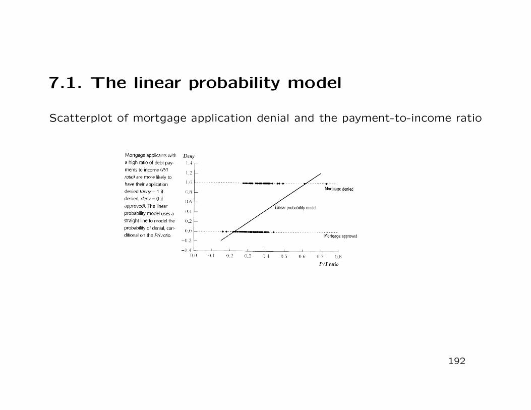
7.1. The linear probability model

Scatterplot of mortgage application denial and the payment-to-income ratio

192

Meaning of the OLS regression line:

• Plot of the predicted value of Y = DENY as a function of theregressor X1 = P/I RATIO

• For example, when P/I RATIO = 0.3 the predicted value ofDENY is 0.2

• General interpretation (for k regressors):

E(Y |X1, . . . , Xk) = 0 · Pr(Y = 0|X1, . . . , Xk)

+1 · Pr(Y = 1|X1, . . . , Xk)

Pr(Y = 1|X1, . . . , Xk)

−→ The predicted value from the regression line is the prob-ability that Y = 1 given the values of the regressorsX1, . . . , Xk

193

Definition 7.1: (Linear probability model)

The linear probability model is the linear multiple regressionmodel

Yi = β0 + β1 ·X1i + . . . + βk ·Xki + ui (7.1)

applied to a binary dependent variable Yi.

Remarks:

• Since Y is binary, it follows that

Pr(Y = 1|X1, . . . , Xk) = β0 + β1 ·X1 + . . . + βk ·Xk

• The coefficient βj is the change in the probability that Y = 1associated with a unit change in Xj holding constant theother regressors

194

Remarks: [continued]

• The regression coefficients can be estimated by OLS

• The errors of the linear probability model are always het-eroskedastic

−→ Use heteroskedasticity-robust standard errors for confi-dence intervals and hypothesis tests

• The R2 is not a useful measure-of-fit(alternative measures-of-fit are discussed later)

195

Application to Boston HMDA data:

• OLS regression of DENY on P/I RATIO yields

DENY = −0.080 + 0.604 · P/I RATIO

(0.032) (0.098)

• Coefficient on DENY is positive and significant at the 1% level

• If P/I RATIO increases by 0.1, the probability of denial in-creases by 0.604× 0.1 ≈ 0.060 = 6%(predicted change in the probability of denial given a changein the regressor)

196

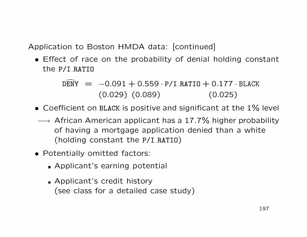
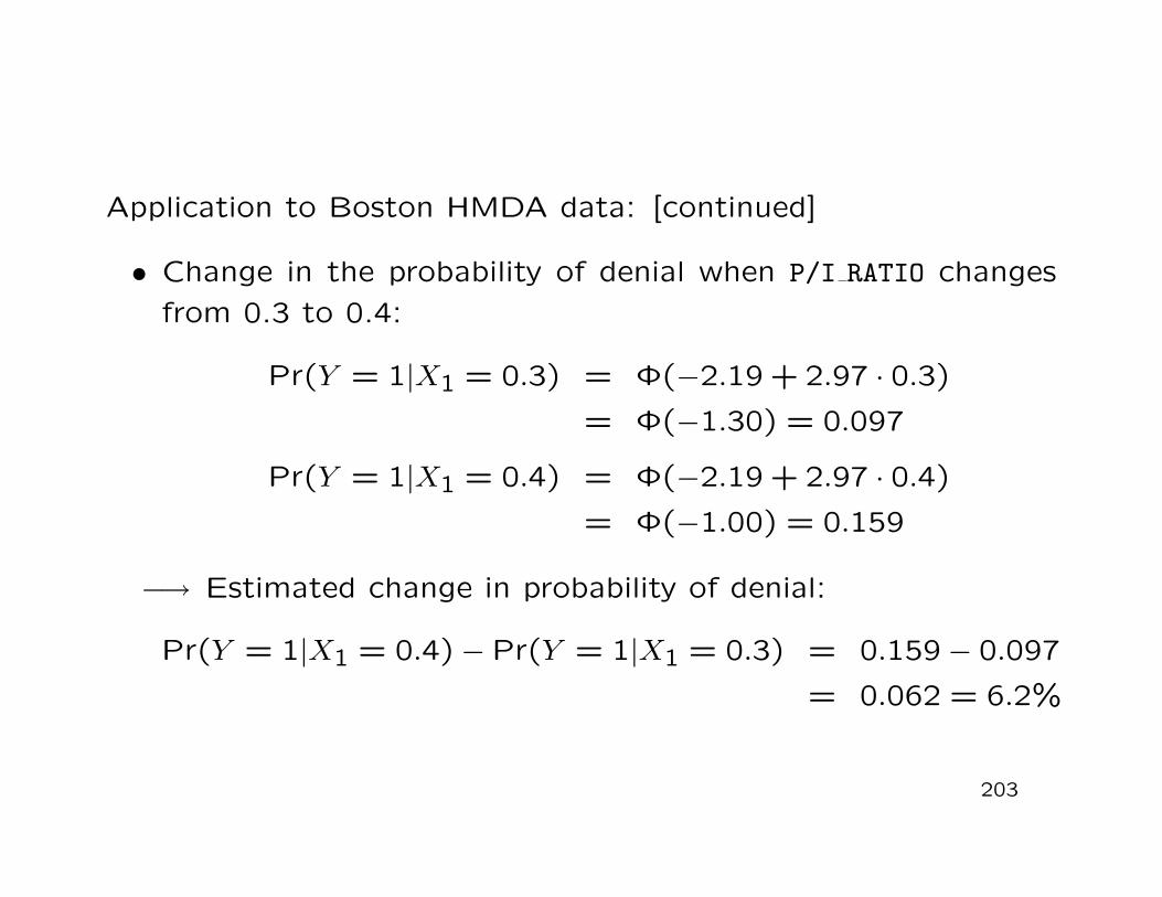
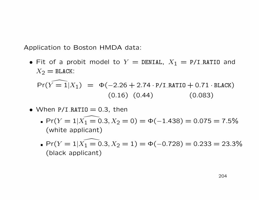
Application to Boston HMDA data: [continued]

• Effect of race on the probability of denial holding constantthe P/I RATIO

DENY = −0.091 + 0.559 · P/I RATIO+ 0.177 · BLACK(0.029) (0.089) (0.025)

• Coefficient on BLACK is positive and significant at the 1% level

−→ African American applicant has a 17.7% higher probabilityof having a mortgage application denied than a white(holding constant the P/I RATIO)

• Potentially omitted factors:

Applicant’s earning potential

Applicant’s credit history(see class for a detailed case study)

197

Major shortcoming of the linear probability model:

• Probabilities cannot fall below 0 or exceed 1

−→ Effect on Pr(Y = 1) of a given change in X must benonlinear

198

7.2. Probit and logit regression

Now:

• Two alternative nonlinear formulations that force the pre-dicted probabilities Pr(Y = 1|X1, . . . , Xk) to range between 0and 1

• The probit regression model uses the standard normal cumu-lative distribution function (cdf)

• The logit regression model uses the logistic cdf

199

Probit model of the probability of DENY, given P/I RATIO

200

Definition 7.2: (Probit regression model)

The population probit model with multiple regressors is given by

Pr(Y = 1|X1, . . . , Xk) = Φ(β0 + β1 ·X1 + . . . + βk ·Xk), (7.2)

where the dependent variable Y is binary, Φ(·) is the cumulativestandard normal distribution function, and X1, . . . , Xk are theregressors.

Remarks:

• The effect on the predicted probability of a change in a re-gressor is obtained by computing the predicted probabilities

1. for the initial Xj-value

2. for the changed Xj-value

3. and by taking their difference

201

Remarks: [continued]

• The probit coefficients and the standard errors are typicallyestimated using the method of maximum likelihood (MLE)(see Section 7.3)

Application to Boston HMDA data:

• Fit of a probit model to Y = DENIAL and X1 = P/I RATIO:

Pr(Y = 1|X1) = Φ(−2.19 + 2.97 · P/I RATIO)

(0.16) (0.47)

• P/I RATIO is positively related to the probability of denial

• Relationship is statistically significant at the 1% level(t-statistic = 2.97/0.47 = 6.32)

202

Application to Boston HMDA data: [continued]

• Change in the probability of denial when P/I RATIO changesfrom 0.3 to 0.4:

Pr(Y = 1|X1 = 0.3) = Φ(−2.19 + 2.97 · 0.3)

= Φ(−1.30) = 0.097

Pr(Y = 1|X1 = 0.4) = Φ(−2.19 + 2.97 · 0.4)

= Φ(−1.00) = 0.159

−→ Estimated change in probability of denial:

Pr(Y = 1|X1 = 0.4)− Pr(Y = 1|X1 = 0.3) = 0.159− 0.097

= 0.062 = 6.2%

203

Application to Boston HMDA data:

• Fit of a probit model to Y = DENIAL, X1 = P/I RATIO andX2 = BLACK:

Pr(Y = 1|X1) = Φ(−2.26 + 2.74 · P/I RATIO+ 0.71 · BLACK)(0.16) (0.44) (0.083)

• When P/I RATIO = 0.3, then

Pr(Y = 1|X1 = 0.3, X2 = 0) = Φ(−1.438) = 0.075 = 7.5%(white applicant)

Pr(Y = 1|X1 = 0.3, X2 = 1) = Φ(−0.728) = 0.233 = 23.3%(black applicant)

204

Definition 7.3: (Logit regression model)

The population logit model with multiple regressors is given by

Pr(Y = 1|X1, . . . , Xk) = F (β0 + β1 ·X1 + . . . + βk ·Xk), (7.3)

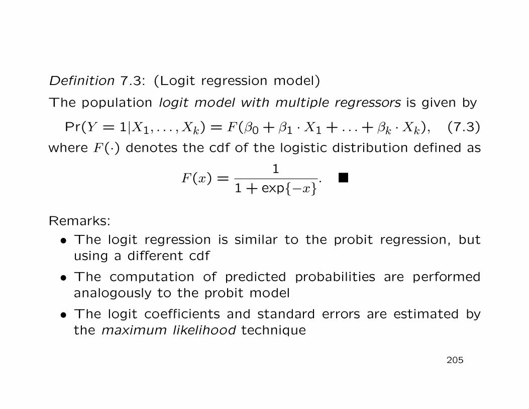
where F (·) denotes the cdf of the logistic distribution defined as

F (x) =1

1 + exp{−x}.

Remarks:• The logit regression is similar to the probit regression, but

using a different cdf

• The computation of predicted probabilities are performedanalogously to the probit model

• The logit coefficients and standard errors are estimated bythe maximum likelihood technique

205

Remarks: [continued]

• In practice, logit and probit regressions often produce similarresults

Probit and logit models of the probability of DENY, given P/I RATIO

206

7.3. Estimation and inference in the logit andprobit models

Alternative estimation techniques:

• Nonlinear least squares estimation by minimizing the sum ofsquared prediction mistakes:

n∑

i=1[Yi −Φ(b0 + b1X1i + . . . + bkXki)]

2 −→ minb0,...,bk

(7.4)

(see Eq. (2.2) on Slide 12)

• Maximum likelihood estimation

207

Nonlinear least squares estimation:

• NLS estimators are

consistent

normally distributed in large samples

• However, NLS estimators are inefficient, that is there areother estimators having a smaller variance than the NLS es-timators

−→ Use of maximum likelihood estimators

208

Maximum likelihood estimation:

• ML estimators are

consistent

normally distributed in large samples

• More efficient than NLS estimators

• ML estimation is discussed in the lecture Advanced Statistics

Statistical inference based on MLE:

• Since ML estimators are normally distributed in large sam-ples, statistical inference about probit and logit coefficientsbased on MLE proceeds in the same way as inference aboutthe linear regression functions coefficients based on the OLSestimator

209

In particular:

• Hypothesis tests are performed using the t- and F -statistics(see Sections 3.2.–3.4.)

• Confidence intervals are constructed according to Formula(3.3) on Slide 55

Measures-of-fit:

• The conventional R2 is inappropriate for probit and logit re-gression models

• Two frequently encountered measures-of-fit with binary de-pendent variables are the

Fraction correctly predicted

Pseudo-R2

210

Fraction correctly predicted:

• This measure-of-fit is based on a simple classification rule

• An observation Yi is said to be correctly predicted,

if Yi = 1 and Pr(Yi = 1|X1i, . . . , Xki) > 0.5 or

if Yi = 0 and Pr(Yi = 1|X1i, . . . , Xki) < 0.5

• Otherwise Yi is said to be incorrectly predicted

• The fraction correctly predicted is the fraction of the n ob-servations Y1, . . . , Yn that are correctly predicted

Pseudo-R2:

• The Pseudo-R2 compares values of the maximized likelihood-function with all regressors to the value of the likelihoodfunction with no regressor

211

Case study:

• Application to Boston HMDA data(see class)

Other limited dependent variable models:

• Censored and truncated regression models

• Sample selection models

• Count data

• Ordered responses

• Discrete choice data

• For details see Ruud (2000) and Wooldridge (2002)

212