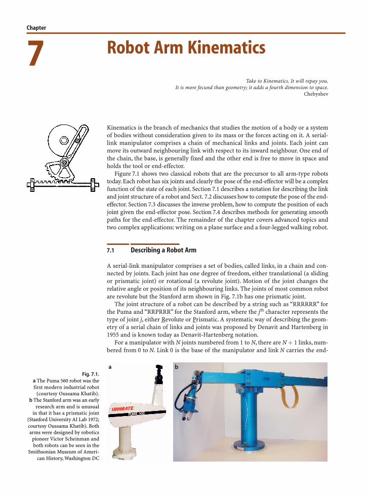
7 Chapter Kinematics is the branch of mechanics that studies the motion of a body or a system of bodies without consideration given to its mass or the forces acting on it. A serial- link manipulator comprises a chain of mechanical links and joints. Each joint can move its outward neighbouring link with respect to its inward neighbour. One end of the chain, the base, is generally fixed and the other end is free to move in space and holds the tool or end-effector. Figure 7.1 shows two classical robots that are the precursor to all arm-type robots today. Each robot has six joints and clearly the pose of the end-effector will be a complex function of the state of each joint. Section 7.1 describes a notation for describing the link and joint structure of a robot and Sect. 7.2 discusses how to compute the pose of the end- effector. Section 7.3 discusses the inverse problem, how to compute the position of each joint given the end-effector pose. Section 7.4 describes methods for generating smooth paths for the end-effector. The remainder of the chapter covers advanced topics and two complex applications: writing on a plane surface and a four-legged walking robot. 7.1 l Describing a Robot Arm A serial-link manipulator comprises a set of bodies, called links, in a chain and con- nected by joints. Each joint has one degree of freedom, either translational (a sliding or prismatic joint) or rotational (a revolute joint). Motion of the joint changes the relative angle or position of its neighbouring links. The joints of most common robot are revolute but the Stanford arm shown in Fig. 7.1b has one prismatic joint. The joint structure of a robot can be described by a string such as “RRRRRR” for the Puma and “RRPRRR” for the Stanford arm, where the j th character represents the type of joint j, either Revolute or Prismatic. A systematic way of describing the geom- etry of a serial chain of links and joints was proposed by Denavit and Hartenberg in 1955 and is known today as Denavit-Hartenberg notation. For a manipulator with N joints numbered from 1 to N, there are N + 1 links, num- bered from 0 to N. Link 0 is the base of the manipulator and link N carries the end- Robot Arm Kinematics Take to Kinematics. It will repay you. It is more fecund than geometry; it adds a fourth dimension to space. Chebyshev Fig. 7.1. a The Puma 560 robot was the first modern industrial robot (courtesy Oussama Khatib). b The Stanford arm was an early research arm and is unusual in that it has a prismatic joint (Stanford University AI Lab 1972; courtesy Oussama Khatib). Both arms were designed by robotics pioneer Victor Scheinman and both robots can be seen in the Smithsonian Museum of Ameri- can History, Washington DC
Transcript
7Chapter
Kinematics is the branch of mechanics that studies the motion of a body or a systemof bodies without consideration given to its mass or the forces acting on it. A serial-link manipulator comprises a chain of mechanical links and joints. Each joint canmove its outward neighbouring link with respect to its inward neighbour. One end ofthe chain, the base, is generally fixed and the other end is free to move in space andholds the tool or end-effector.
Figure 7.1 shows two classical robots that are the precursor to all arm-type robotstoday. Each robot has six joints and clearly the pose of the end-effector will be a complexfunction of the state of each joint. Section 7.1 describes a notation for describing the linkand joint structure of a robot and Sect. 7.2 discusses how to compute the pose of the end-effector. Section 7.3 discusses the inverse problem, how to compute the position of eachjoint given the end-effector pose. Section 7.4 describes methods for generating smoothpaths for the end-effector. The remainder of the chapter covers advanced topics andtwo complex applications: writing on a plane surface and a four-legged walking robot.
7.1 lDescribing a Robot Arm
A serial-link manipulator comprises a set of bodies, called links, in a chain and con-nected by joints. Each joint has one degree of freedom, either translational (a slidingor prismatic joint) or rotational (a revolute joint). Motion of the joint changes therelative angle or position of its neighbouring links. The joints of most common robotare revolute but the Stanford arm shown in Fig. 7.1b has one prismatic joint.
The joint structure of a robot can be described by a string such as “RRRRRR” forthe Puma and “RRPRRR” for the Stanford arm, where the jth character represents thetype of joint j, either Revolute or Prismatic. A systematic way of describing the geom-etry of a serial chain of links and joints was proposed by Denavit and Hartenberg in1955 and is known today as Denavit-Hartenberg notation.
For a manipulator with N joints numbered from 1 to N, there are N+ 1 links, num-bered from 0 to N. Link 0 is the base of the manipulator and link N carries the end-
Robot Arm Kinematics
Take to Kinematics. It will repay you.It is more fecund than geometry; it adds a fourth dimension to space.
Chebyshev
Fig. 7.1.a The Puma 560 robot was thefirst modern industrial robot
(courtesy Oussama Khatib).b The Stanford arm was an early
research arm and is unusualin that it has a prismatic joint
(Stanford University AI Lab 1972;courtesy Oussama Khatib). Botharms were designed by robotics
pioneer Victor Scheinman andboth robots can be seen in the
Smithsonian Museum of Ameri-can History, Washington DC
138
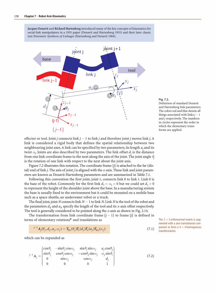
effector or tool. Joint j connects link j− 1 to link j and therefore joint j moves link j. Alink is considered a rigid body that defines the spatial relationship between twoneighbouring joint axes. A link can be specified by two parameters, its length aj and itstwist αj. Joints are also described by two parameters. The link offset dj is the distancefrom one link coordinate frame to the next along the axis of the joint. The joint angle θjis the rotation of one link with respect to the next about the joint axis.
Figure 7.2 illustrates this notation. The coordinate frame {j} is attached to the far (dis-tal) end of link j. The axis of joint j is aligned with the z-axis. These link and joint param-eters are known as Denavit-Hartenberg parameters and are summarized in Table 7.1.
Following this convention the first joint, joint 1, connects link 0 to link 1. Link 0 isthe base of the robot. Commonly for the first link d1=α1= 0 but we could set d1> 0to represent the height of the shoulder joint above the base. In a manufacturing systemthe base is usually fixed to the environment but it could be mounted on a mobile basesuch as a space shuttle, an underwater robot or a truck.
The final joint, joint N connects link N− 1 to link N. Link N is the tool of the robot andthe parameters dN and aN specify the length of the tool and its x-axis offset respectively.The tool is generally considered to be pointed along the z-axis as shown in Fig. 2.14.
The transformation from link coordinate frame {j− 1} to frame {j} is defined interms of elementary rotations� and translations as
(7.1)
which can be expanded as
(7.2)
Fig. 7.2.Definition of standard Denavitand Hartenberg link parameters.The colors red and blue denote allthings associated with links j− 1and j respectively. The numbersin circles represent the order inwhich the elementary trans-forms are applied
Jacques Denavit and Richard Hartenberg introduced many of the key concepts of kinematics forserial-link manipulators in a 1955 paper (Denavit and Hartenberg 1955) and their later classictext Kinematic Synthesis of Linkages (Hartenberg and Denavit 1964).
The 3× 3 orthonormal matrix is aug-mented with a zero translational com-ponent to form a 4× 4 homogenoustransformation.
Chapter 7 · Robot Arm Kinematics
139
The parameters αj and aj are always constant. For a revolute joint θj is the joint vari-able and dj is constant, while for a prismatic joint dj is variable, θj is constant and αj= 0.In many of the formulations that follow we use generalized joint coordinates
For an N-axis robot the generalized joint coordinates q ∈ C where C⊂RN is calledthe joint space or configuration space.� For the common case of an all-revolute robotC⊂ SN the joint coordinates are referred to as joint angles. The joint coordinates arealso referred to as the pose of the manipulator which is different to the pose of theend-effector which is a Cartesian pose ξ ∈ SE(3). The term configuration is shorthandfor kinematic configuration which will be discussed in Sect. 7.3.1.
Within the Toolbox we represent a robot link with a Link object which is created by
where the elements of the input vector are given in the order θk, dj, aj, αj. The optionalfifth element σj indicates whether the joint is revolute (σi= 0) or prismatic (σi= 0). Ifnot specified a revolute joint is assumed.
The displayed values of the Link object shows its kinematic parameters as well asother status such the fact that it is a revolute joint (the tag R) and that the standardDenavit-Hartenberg parameter convention is used (the tag stdDH).�
Although a value was given for θ it is not displayed – that value simply servedas a placeholder in the list of kinematic parameters. θ is substituted by the jointvariable q and its value in the Link object is ignored. The value will be man-aged by the Link object.
A Link object has many parameters and methods which are described in the onlinedocumentation, but the most common ones are illustrated by the following examples.The link transform Eq. 7.2 for q= 0.5 rad is
Table 7.1.Denavit-Hartenberg parameters:
their physical meaning, symboland formal definition
Jacques Denavit (1930–) was born in Paris where he studied for his Bachelor degree beforepursuing his masters and doctoral degrees in mechanical engineering at Northwestern Univer-sity, Illinois. In 1958 he joined the Department of Mechanical Engineering and AstronauticalScience at Northwestern where the collaboration with Hartenberg was formed. In addition tohis interest in dynamics and kinematics Denavit was also interested in plasma physics andkinetics. After the publication of the book he moved to Lawrence Livermore National Lab,Livermore, California, where he undertook research on computer analysis of plasma physicsproblems. He retired in 1982.
This is the same concept as was intro-duced for mobile robots on page 65.
A slightly different notation, modifedDenavit-Hartenberg notation is dis-cussed in Sect. 7.5.3.
which is added to the joint variable before computing the link transform and will bediscussed in more detail in Sect. 7.5.1.
7.2 lForward Kinematics
The forward kinematics is often expressed in functional form
(7.3)
with the end-effector pose as a function of joint coordinates. Using homogeneous trans-formations this is simply the product of the individual link transformation matricesgiven by Eq. 7.2 which for an N-axis manipulator is
(7.4)
The forward kinematic solution can be computed for any serial-link manipulatorirrespective of the number of joints or the types of joints. Determining the Denavit-Hartenberg parameters for each of the robot’s links is described in more detail inSect. 7.5.2.
The pose of the end-effector ξE∼ TE∈ SE(3) has six degrees of freedom – three intranslation and three in rotation. Therefore robot manipulators commonly have sixjoints or degrees of freedom to allow them to achieve an arbitrary end-effector pose.The overall manipulator transform is frequently written as T6 for a 6-axis robot.
Richard Hartenberg (1907–1997) was born in Chicago and studied for his degrees at the Universityof Wisconsin, Madison. He served in the merchant marine and studied aeronautics for two years atthe University of Goettingen with space-flight pioneer Theodor von Karman. He was Professor ofmechanical engineering at Northwestern University where he taught for 56 years. His research inkinematics led to a revival of interest in this field in the 1960s, and his efforts helped put kinemat-ics on a scientific basis for use in computer applications in the analysis and design of complexmechanisms. His also wrote extensively on the history of mechanical engineering.
Chapter 7 · Robot Arm Kinematics
141
7.2.1 lA 2-Link Robot
The first robot that we will discuss is the two-link planar manipulator shown in Fig. 7.3.It has the following Denavit-Hartenberg parameterswhich we use to create a vector of Link objects
This provides a concise description of the robot. We see that it has 2 revolute joints asindicated by the structure string 'RR', it is defined in terms of standard Denavit-Hartenberg parameters, that gravity is acting in the default z-direction.� The kine-matic parameters of the link objects are also listed and the joint variables are shown asvariables q1 and q2. We have also assigned a name to the robot which will be shownwhenever the robot is displayed graphically. The script
>> mdl_twolink
performs the above steps and defines this robot in the MATLAB® workspace, creatinga SerialLink object named twolink.
The SerialLink object is key to the operation of the Robotics Toolbox. It has agreat many methods and properties which are illustrated in the rest of this part, anddescribed in detail in the online documentation. Some simple examples are
the method returns the homogenous transform that represents the pose of thesecond link coordinate frame of the robot, T2. For a different configuration thetool pose is
By convention, joint coordinates with the Toolbox are row vectors.
Normal to the plane in which the robotmoves.
Link objects are derived from theMATLAB® handle class and can beset in place. Thus we can write code liketwolink.links(1).a = 2to change the kinematic parameter a2.
A unique name is required when mul-tiple robots are displayed graphically,see Sect. 7.8 for more details.
as stick figures shown in Fig. 7.4. The graphical representation includes the robot’sname, the final-link coordinate frame, T2 in this case, the joints and their axes, and ashadow on the ground plane. Additional features of the plot method such as mul-tiple views and multiple robots are described in Sect. 7.8 with additional details in theonline documentation.
The simple two-link robot introduced above is limited in the poses that it can achievesince it operates entirely within the xy-plane, its task space is T⊂R2.
7.2.2 lA 6-Axis Robot
Truly useful robots have a task space T⊂ SE(3) enabling arbitrary position and atti-tude of the end-effector – the task space has six spatial degrees of freedom: three trans-lational and three rotational. This requires a robot with a configuration space C⊂R6
which can be achieved by a robot with six joints. In this section we will use the Puma 560as an example of the class of all-revolute six-axis robot manipulators. We define aninstance of a Puma 560 robot using the script�
>> mdl_puma560
which creates a SerialLink object, p560, in the workspace
Fig. 7.4. The two-link robot in twodifferent poses, a the pose (0, 0);b the pose (ý ,−ý ). Note thegraphical details. Revolute jointsare indicated by cylinders and thejoint axes are shown as line seg-ments. The final-link coordinateframe and a shadow on the groundare also shown
The Toolbox has scripts to define a num-ber of common industrial robots in-cluding the Motoman HP6, Fanuc 10L,ABB S4 2.8 and the Stanford arm.
7.2 · Forward Kinematics
144
Note that aj and dj are in SI units which means that the translational part of the for-ward kinematics will also have SI units.
The script mdl_puma560 also creates a number of joint coordinate vectors in theworkspace which represent the robot in some canonic configurations:
qz (0, 0, 0, 0, 0, 0) zero angleqr (0, ü ,−ü , 0, 0, 0) ready, the arm is straight and verticalqs (0, 0,−ü , 0, 0, 0) stretch, the arm is straight and horizontalqn (0, ý ,−π, 0, ý , 0) nominal, the arm is in a dextrous working pose�
and these are shown graphically in Fig. 7.5. These plots are generated using the plotmethod, for example
>> p560.plot(qz)
The Puma 560 robot (Programmable Universal Manipulator for Assembly) shown in Fig. 7.1 wasreleased in 1978 and became enormously popular. It featured an anthropomorphic design, elec-tric motors and a spherical wrist which makes it the first modern industrial robot – the archetypeof all that followed.
The Puma 560 catalyzed robotics research in the 1980s and it was a very common laboratoryrobot. Today it is obsolete and rare but in homage to its important role in robotics researchwe use it here. For our purposes the advantages of this robot are that it has been well studiedand its parameters are very well known – it has been described as the “white rat” of roboticsresearch.
Most modern 6-axis industrial robots are very similar in structure and can be accomodatedsimply by changing the Denavit-Hartenberg parameters. The Toolbox has kinematic models fora number of common industrial robots including the Motoman HP6, Fanuc 10L, and ABB S4 2.8.
Fig. 7.5. The Puma robot in 4 dif-ferent poses. a Zero angle; b readypose; c stretch; d nominal
Well away from singularities, which willbe discussed in Sect. 7.4.3.
which returns the homogeneous transformation corresponding to the end-effectorpose T6. The origin of this frame, the link 6 coordinate frame {6}, is defined� as thepoint of intersection of the axes of the last 3 joints – physically this point is inside therobot’s wrist mechanism. We can define a tool transform, from the T6 frame to theactual tool tip by
>> p560.tool = transl(0, 0, 0.2);
in this case a 200 mm extension in the T6 z-direction.� The pose of the tool tip, oftenreferred to as the tool centre point or TCP, is now
The kinematic definition we have used considers that the base of the robot is the inter-section point of the waist and shoulder axes which is a point inside the structure of therobot. The Puma 560 robot includes a 30 inch tall pedestal. We can shift the origin of therobot from the point inside the robot to the base of the pedestal using a base transform
>> p560.base = transl(0, 0, 30*0.0254);
where for consistency we have converted the pedestal height to SI units. Now, withboth base and tool transform, the forward kinematics are
which positions the robot’s origin 3 m above the world origin with its coordinate framerotated by 180° about the x-axis. This robot is now hanging from the ceiling!
Anthropomorphic means having human-like characteristics. The Puma 560 robot was designedto have approximately the dimensions and reach of a human worker. It also had a spherical jointat the wrist just as humans have.
Roboticists also tend to use anthropomorphic terms when describing robots. We use wordslike waist, shoulder, elbow and wrist when describing serial link manipulators. For the Pumathese terms correspond respectively to joint 1, 2, 3 and 4–6.
By the mdl_puma560 script.
Alternatively we could change the ki-nematic parameter d6. The tool trans-form approach is more general sincethe final link kinematic parameters onlyallow setting of d6, a6 and α 6 whichprovide z-axis translation, x-axis trans-lation and x-axis rotation respectively.
7.2 · Forward Kinematics
146
The Toolbox supports joint angle time series or trajectories such as
where each row represents the joint coordinates at a different timestep and the col-umns represent the joints.� In this case the method fkine
>> T = p560.fkine(q);
returns a 3-dimensional matrix
>> about(T)T [double] : 4x4x8 (1024 bytes)
where the first two dimensions are a 4× 4 homogeneous transformation and the thirddimension is the timestep. The homogeneous transform corresponding to the jointcoordinates in the fourth row of q is
We have shown how to determine the pose of the end-effector given the joint coordi-nates and optional tool and base transforms. A problem of real practical interest is theinverse problem: given the desired pose of the end-effector ξE what are the requiredjoint coordinates? For example, if we know the Cartesian pose of an object, what jointcoordinates does the robot need in order to reach it? This is the inverse kinematicsproblem which is written in functional form as
(7.5)
In general this function is not unique and for some classes of manipulator no closed-form solution exists, necessitating a numerical solution.
7.3.1 lClosed-Form Solution
A necessary condition for a closed-form solution of a 6-axis robot is that the threewrist axes intersect at a single point. This means that motion of the wrist joints onlychanges the end-effector orientation, not its translation. Such a mechanism is knownas a spherical wrist and almost all industrial robots have such wrists.
We will explore inverse kinematics using the Puma robot model
>> mdl_puma560
Generated by the jtraj function,which is discussed in Sect. 7.4.1.
Chapter 7 · Robot Arm Kinematics
147
At the nominal joint coordinates>> qnqn = 0 0.7854 3.1416 0 0.7854 0
Since the Puma 560 is a 6-axis robot arm with a spherical wrist we use the methodikine6s to compute the inverse kinematics using a closed-form solution.� The re-quired joint coordinates to achieve the pose T are
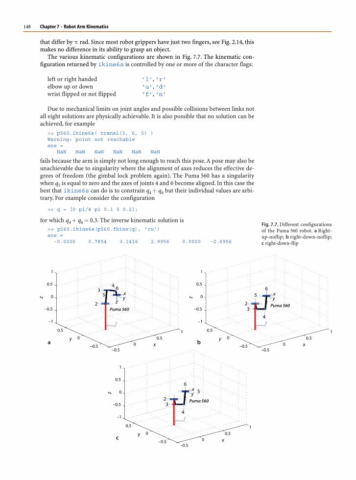
we see that these two different sets of joint coordinates result in the same end-effectorpose and these are shown in Fig. 7.6. The shoulder of the Puma robot is horizontallyoffset from the waist, so in one solution the arm is to the left of the waist, in the otherit is to the right. These are referred to as the left- and right-handed kinematic con-figurations respectively. In general there are eight sets of joint coordinates that givethe same end-effector pose – as mentioned earlier the inverse solution is not unique.
We can force the right-handed solution>> qi = p560.ikine6s(T, 'ru')qi = -0.0000 0.7854 3.1416 0.0000 0.7854 -0.0000
which gives the original set of joint angles by specifying a right handed configurationwith the elbow up.
In addition to the left- and right-handed solutions, there are solutions with theelbow either up or down,� and with the wrist flipped or not flipped. For the Puma 560robot the wrist joint, θ4, has a large rotational range and can adopt one of two angles
Fig. 7.6. Two solutions to the in-verse kinematic problem, left-handed and right-handed solu-tions. The shadow shows clearlythe two different configurations
The method ikine6s checks the De-navit-Hartenberg parameters to deter-mine if the robot meets these criteria.
More precisely the elbow is above or be-low the shoulder.
7.3 · Inverse Kinematics
148
that differ by π rad. Since most robot grippers have just two fingers, see Fig. 2.14, thismakes no difference in its ability to grasp an object.
The various kinematic configurations are shown in Fig. 7.7. The kinematic con-figuration returned by ikine6s is controlled by one or more of the character flags:
left or right handed 'l', 'r'elbow up or down 'u', 'd'wrist flipped or not flipped 'f', 'n'
Due to mechanical limits on joint angles and possible collisions between links notall eight solutions are physically achievable. It is also possible that no solution can beachieved, for example
>> p560.ikine6s( transl(3, 0, 0) )Warning: point not reachableans = NaN NaN NaN NaN NaN NaN
fails because the arm is simply not long enough to reach this pose. A pose may also beunachievable due to singularity where the alignment of axes reduces the effective de-grees of freedom (the gimbal lock problem again). The Puma 560 has a singularitywhen q5 is equal to zero and the axes of joints 4 and 6 become aligned. In this case thebest that ikine6s can do is to constrain q4+ q6 but their individual values are arbi-trary. For example consider the configuration
>> q = [0 pi/4 pi 0.1 0 0.2];
for which q4+ q6= 0.3. The inverse kinematic solution is>> p560.ikine6s(p560.fkine(q), 'ru')ans = -0.0000 0.7854 3.1416 2.9956 0.0000 -2.6956
Fig. 7.7. Different configurationsof the Puma 560 robot. a Right-up-noflip; b right-down-noflip;c right-down-flip
Chapter 7 · Robot Arm Kinematics
149
has quite different values for q4 and q6 but their sum>> q(4)+q(6)ans = 0.3000
remains the same.
7.3.2 lNumerical Solution
For the case of robots which do not have six joints and a spherical wrist we need to usean iterative numerical solution. Continuing with the example of the previous sectionwe use the method ikine to compute the general inverse kinematic solution
which is different to the original value>> qnqn = 0 0.7854 3.1416 0 0.7854 0
but does result in the correct tool pose>> p560.fkine(qi)ans = -0.0000 0.0000 1.0000 0.5963 -0.0000 1.0000 -0.0000 -0.1501 -1.0000 -0.0000 -0.0000 -0.0144 0 0 0 1.0000
Plotting the pose
>> p560.plot(qi)
shows clearly that ikine has found the elbow-down configuration.A limitation of this general numeric approach is that it does not provide explicit
control over the arm’s kinematic configuration as did the analytic approach – the onlycontrol is implicit via the initial value of joint coordinates (which defaults to zero). Ifwe specify the initial joint coordinates
the solution converges on the elbow-up configuration.�
As would be expected the general numerical approach of ikine is considerably slowerthan the analytic approach of ikine6s. However it has the great advantage of beingable to work with manipulators at singularities and manipulators with less than six ormore than six joints. Details of the principle behind ikine is provided in Sect. 8.4.
7.3.3 lUnder-Actuated Manipulator
An under-actuated manipulator is one that has fewer than six joints, and is thereforelimited in the end-effector poses that it can attain. SCARA robots such as shown on page 135are a common example, they have typically have an x-y-z-θ task space, T⊂R3
× S
and a configuration space C⊂ S3×R.
7.3 · Inverse Kinematics
When solving for a trajectory as on p. 146the inverse kinematic solution for onepoint is used to initialize the solutionfor the next point on the path.
150
We will revisit the two-link manipulator example from Sect. 7.2.1, first defining the robot
>> mdl_twolink
and then defining the desired end-effector pose
>> T = transl(0.4, 0.5, 0.6);
However this pose is over-constrained for the two-link robot – the tool cannot meetthe orientation constraint on the direction of '2 and (2 nor a z-axis translationalvalue other than zero. Therefore we require the ikine method to consider only er-ror in the x- and y-axis translational directions, and ignore all other Cartesian de-grees of freedom. We achieve this by specifying a mask vector as the fourth argument
The elements of the mask vector correspond respectively to the three translationsand three orientations: tx, ty, tz, rx, ry, rz in the end-effector coordinate frame. In thisexample we specified that only errors in x- and y-translation are to be considered(the non-zero elements). The resulting joint angles correspond to an endpoint pose
which has the desired x- and y-translation, but the orientation and z-translation areincorrect, as we allowed them to be.
7.3.4 lRedundant Manipulator
A redundant manipulator is a robot with more than six joints. As mentioned previ-ously, six joints is theoretically sufficient to achieve any desired pose in a Cartesiantaskspace T⊂ SE(3). However practical issues such as joint limits and singularitiesmean that not all poses within the robot’s reachable space can be achieved. Addingadditional joints is one way to overcome this problem.
To illustrate this we will create a redundant manipulator. We place our familiarPuma robot
>> mdl_puma560
on a platform that moves in the xy-plane, mimicking a robot mounted on a vehicle. This robothas the same task space T⊂ SE(3) as the Puma robot, but a configuration space C⊂R2
× S6.
The dimension of the configuration space exceeds the dimensions of the task space.The Denavit-Hartenberg parameters for the base are
and using a shorthand syntax we create the SerialLink object directly from theDenavit-Hartenberg parameters
The Denavit-Hartenberg notation requires that prismatic joints cause translation inthe local z-direction and the base-transform rotates that z-axis into the world x-axisdirection. This is a common complexity with Denavit-Hartenberg notation and analternative will be introduced in Sect. 7.5.2.
The joint coordinates of this robot are its x- and y-position and we test that ourDenavit-Hartenberg parameters are correct
We see that the rotation submatrix is the identity matrix, meaning that the coordinateframe of the platform is parallel with the world coordinate frame, and that the x- andy-displacement is as requested.
We mount the Puma robot on the platform by connecting the two robots in series.In the Toolbox we can express this in two different ways, by multiplication
>> p8 = platform * p560;
or by concatenation
p8 = SerialLink( [platform, p560]);
which also allows other attributes of the created SerialLink object to be specified.However there is a small complication. We would like the Puma arm to be sitting on
its tall pedestal on top of the platform. Previously we added the pedestal as a basetransform, but base transforms can only exist at the start of a kinematic chain, and werequire the transform between joints 2 and 3 of the 8-axis robot. Instead we implementthe pedestal by setting d1 of the Puma to the pedestal height
>> p560.links(1).d = 30 * 0.0254;
and now we can compound the two robots>> p8 = SerialLink( [platform, p560], 'name', 'P8')p8 =
resulting in a new 8-axis robot which we have named the P8. We note that the newrobot has inherited the base transform of the platform, and that the pedestal displace-ment appears now as d3.
We can find the inverse kinematics for this new redundant manipulator using thegeneral numerical solution. For example to move the end effector to (0.5, 1.0, 0.7) withthe tool pointing downward in the xz-plane the Cartesian pose is
7.3 · Inverse Kinematics
152
>> T = transl(0.5, 1.0, 0.7) * rpy2tr(0, 3*pi/4, 0);
The first two elements are displacements of the prismatic joints in the base, and thelast six are the robot arm’s joint angles. We see that the solution has made good use ofthe second joint, the platform’s y-axis translation to move the base of the arm close tothe desired point. We can visualize the configuration
>> p8.plot(qi)
which is shown in Fig. 7.8. We can also show that the plain old Puma cannot reach thepoint we specified
>> p560.ikine6s(T)Warning: point not reachable
This robot has 8 degrees of freedom. Intuitively it is more dextrous than its 6-axiscounterpart because there is more than one joint that can contribute to every Carte-sian degree of freedom. This is more formally captured in the notion of manipulabil-ity which we will discuss in Sect. 8.1.4. For now we will consider it as a scalar measurethat reflects the ease with which the manipulator’s tool can move in different Carte-sian directions. The manipulability of the 6-axis robot
>> p560.maniplty(qn)ans = 0.0786
is much less than that for the 8-axis robot>> p8.maniplty([0 0 qn])ans = 1.1151
which indicates the increased dexterity of the 8-axis robot.
7.4 lTrajectories
One of the most common requirements in robotics is to move the end-effector smoothlyfrom pose A to pose B. Building on what we learnt in Sect. 3.1 we will discuss two ap-proaches to generating such trajectories: straight lines in joint space and straight lines inCartesian space. These are known respectively as joint-space and Cartesian motion.