70 IEEE TRANSACTIONS ON VISUALIZATION AND COMPUTER ...mucha/Reprints/TVCGswimming.pdf · HE field...

Fluid Simulation with Articulated BodiesNipun Kwatra, Chris Wojtan, Mark Carlson, Irfan Essa, Senior Member, IEEE,

Peter J. Mucha, and Greg Turk, Member, IEEE

Abstract—We present an algorithm for creating realistic animations of characters that are swimming through fluids. Our approach

combines dynamic simulation with data-driven kinematic motions (motion capture data) to produce realistic animation in a fluid. The

interaction of the articulated body with the fluid is performed by incorporating joint constraints with rigid animation and by extending a

solid/fluid coupling method to handle articulated chains. Our solver takes as input the current state of the simulation and calculates the

angular and linear accelerations of the connected bodies needed to match a particular motion sequence for the articulated body. These

accelerations are used to estimate the forces and torques that are then applied to each joint. Based on this approach, we demonstrate

simulated swimming results for a variety of different strokes, including crawl, backstroke, breaststroke, and butterfly. The ability to have

articulated bodies interact with fluids also allows us to generate simulations of simple water creatures that are driven by simple

controllers.

Index Terms—Physically-based animation, fluid simulation, motion capture.

Ç

1 INTRODUCTION

THE field of computer graphics has recently witnessedsignificant maturity in the use of physics-based simula-

tion and data-driven methods for generating realisticanimations. In part, use of physical simulation has providedfor some very good approaches for animating fluids (see [1],[2], [3], [4] for a review). Character animation either remainsin the hands of talented animators with good tools for keyframing or is performed using data-driven animation.Motion capture technologies are now in wide use to capturedata of performances to animate characters. A major benefitof motion capture is that it provides many of the details andnuances of live motion. The usability of motion capture foranimation has been further enhanced by some practicalapproaches for the adaptation and reuse of alreadycaptured data (see [5], [6], [7], [8]). However, only a fewefforts make the data of character motion interact with thesurrounding physical environment, especially a complexsimulated environment with fluids. For example, it wouldbe interesting to take a kinematic motion of a fish and put itin simulated water to animate the effects that the fish andthe water have on each other. Similarly, it would be of great

benefit for animators if motion capture data of a personperforming swimming actions in the air could be put insimulated water to generate swimming animations, affect-ing both the character and the fluid.

We propose a method for simulating the interactionbetween an articulated character and a simulated fluid.Using our approach, an animator can take any form of motiontrajectory associated with a geometry, either in the form of amotion capture sequence or a related kinematic animation,insert it into a physical simulation of water, and animate theeffects that they have on each other (see Fig. 2). In our method,we use the motion trajectories from an articulated character tocalculate joint forces that closely mimic the input data whenapplied to the physical model. Once we have this simulation ofthe character, we make it interact with the fluid. To achievethis interaction, we turn to some of the recent efforts onsimulating two-way interactions between rigid bodies andfluids. Specifically, we build on the Rigid Fluid method for fulltwo-way coupling between the rigid bodies and fluids [9]. Aswe are interested in articulated character animations, weneed to extend the Rigid Fluid approach to incorporate rigidbodies with joints.

Our method consists of two main steps:

1. Force/torque extraction: Given motion capture data,we calculate the forces and torques that must beapplied to our articulated body joints duringsimulation so that it follows the motion capture dataas closely as possible. We use a constraint-basedmethod discussed in Section 3, for this purpose.

2. Fluid-body coupling: Once we have the joint forcesand torques, we simulate the articulated body in thefluid environment using our extension of the RigidFluid method. This interaction changes the fluidenvironment (e.g., creates splashes) and also affectsthe articulated body simulation (e.g., a person doinga swimming action is pushed forward).

The above two steps are repeated to form a feedbackmechanism. The overall flow diagram of our approach isshown in Fig. 1. The forces due to fluid/body coupling may

70 IEEE TRANSACTIONS ON VISUALIZATION AND COMPUTER GRAPHICS, VOL. 16, NO. 1, JANUARY/FEBRUARY 2010

. N. Kwatra is with Stanford University, 353 Serra Mall, Stanford, CA94305-9020. E-mail: [email protected].

. C. Wojtan is with the Georgia Institute of Technology, 709B Penn Ave,Atlanta, GA 30308. E-mail: [email protected].

. M. Carlson is with DreamWorks Animation, 315 Palo Alto Ave, MountainView, CA 94041. E-mail: [email protected].

. I. Essa and G. Turk are with the School of Interactive Computing, GeorgiaInstitute of Technology, 85 5th Street NW, Atlanta, GA 30332-0760.E-mail: [email protected], [email protected].

. P.J. Mucha is with Carolina Center for Interdisciplinary AppliedMathematics, Department of Mathematics & Institute for AdvancedMaterials, Nanoscience, and Technology, University of North Carolina,Chapel Hill, NC 27599-3250. E-mail: [email protected].

Manuscript received 12 Jan. 2009; revised 17 Apr. 2009; accepted 26 May2009; published online 10 June 2009.Recommended for acceptance by S.Y. Shin.For information on obtaining reprints of this article, please send e-mail to:[email protected], and reference IEEECS Log Number TVCG-2009-01-0009.Digital Object Identifier no. 10.1109/TVCG.2009.66.

1077-2626/10/$26.00 � 2010 IEEE Published by the IEEE Computer Society

Authorized licensed use limited to: University of North Carolina at Chapel Hill. Downloaded on December 10, 2009 at 13:11 from IEEE Xplore. Restrictions apply.

cause the simulation to deviate from the motion capturedata, but the force/torque extraction step tries to bring thearticulated figure back into step with the data. Thus, theswimmer closely follows the motion capture data in terms ofthe relative joint angles, but at the same time is given a globaltranslation and rotational motion that represents the netforce and torque from the fluid to the swimmer. Thiscompletes the two-way coupling of the swimmer with thefluid environment.

Our work broadens the range of objects that can interactwith simulated fluids. In prior work, examples have beencreated in which a ball or feet have caused splashes in fluids[1], [2], [10]. In such cases, the trajectory of the ball is notaffected by the fluid. Examples have also been created thatsimulate buoyant objects that are floating on the surface of thewater [11]. In these situations, the object does not cause anychange to the water. Only recently have we seen animationswhere the motion of the object affects the fluid and vice versa[3], [9], [12], [13], [14], [15], [16], [17]. We use a full two-waysolid-fluid coupling enabling us to demonstrate effects thatwere not viable before. For example, the two-way simulationallows us to simulate surface effects like splashing whileimpacting the motion of the object in the fluid. Our articulatedstructures impart complex forces on the fluid and in returnthe fluid propels the structure in the ways that we expect.Using our approach, we are able to dynamically simulatecharacters swimming in water. Using a simple controller, wealso demonstrate the validity of a result due to Purcell aboutsimple swimmers at low Reynolds numbers [18].

2 RELATED WORK

Most of the work in motion capture research is focused onreusing already captured data either to synthesize newanimation by copying pieces from a database and reassem-bling them, or to generate new motions by using kinematicsconstraint satisfaction to search for new variations onexisting data. Recently, however, some researchers havetried to combine motion capture and simulation so thatmotion captured characters can dynamically interact with aphysically simulated environment.

Oshita and Makinouchi [19] use simulation to allow acharacter to respond to a mass being dropped on its back.

Zordan and Hodgins [20] create simulations from motioncapture data that are able to hit and react to collisions. Thiswork is closest to ours in spirit. They choose to model motioncapture data with proportional-derivative (PD) servos, andallow passive dynamics to take over during impacts. Thestiffness parameters of the servo are interpolated to smoothlyswitch between tracking and passive control. Unlike thistransition between tracking motion capture data and passivedynamics, since we are interested in interacting with fluids,our articulated figure is continuously interacting with thephysical environment at all times.

Recently, Yang et al. [21] developed a layered strategy tocontrol swimming motions. In their approach, they employa simple viscous drag model and do not perform a full fluidsimulation. They specifically state that “A full CFD[computational fluid dynamics] with unsteady flow is,however, necessary to truly capture the motion of swim-ming characters.” [21]. MacIver et al. [22] demonstratecoupling of the fluid with flexible bodies, with details to bepublished, including results for simulating free swimmingmotion of fish in a viscous fluid.

Previous works on characters that interact with fluidsuse simple models for calculating forces between fluid andsolids. Tu and Terzopoulos [23] compute forces on a fishsurface using the surface normal and relative velocitybetween the surface and water. Their simulation does notaffect the water at all, and hence, surface phenomena likesplashing could not be demonstrated. Along the same lines,Wu and Popovic [24] use a simple model of aerodynamicsto create the lift and drag forces on birds.

Several methods have been used in graphics to allowmodeling of full two-way coupling between fluids andsolids. Yngve et al. [25] simulate destructive explosions withtwo-way coupling of breakable rigid bodies and compres-sible high-speed fluid. Genevaux et al. [12] implement two-way coupling between incompressible fluid and deformablesolids modeled by mass/spring systems. Takahashi et al.[26], [27] model the interaction of incompressible fluids andrigid bodies by setting the velocity of the rigid body asboundary conditions to the fluid solver, and using the fluid’spressure to calculate a normal force acting on the surface ofthe rigid body. Guendelman et al. [13] use a similar objectvelocity/fluid pressure coupling to animate the interactionof incompressible fluids with zero volume deformable andrigid shells. Robinson-Mosher et al. [3], Klingner et al. [15],Chentanez et al. [16], and Batty et al. [17] solve simulta-neously for the fluid pressure and solid velocity to obtain afully implicit two-way solid-fluid coupling. We chose to usethe Rigid Fluid method from Carlson et al. [9] to model ourrigid bodies interacting with incompressible fluid. Thismethod affords an easy translation of forces between the

KWATRA ET AL.: FLUID SIMULATION WITH ARTICULATED BODIES 71

Fig. 1. Flow diagram of our approach.

Fig. 2. A simulated swimmer that is driven by motion capture data. The

forward motion of the swimmer is due to the interactions between the

figure and the simulated fluid.


simulations and was straightforward to implement. Themethod scales linearly, and it adds very little overheadcompared to the cost of the fluid simulation. We recognizethat other coupling techniques for solid/fluid interactionsuch as [3] may also be appropriate for our goals. We believethat our constraint-based solver will work equally well withthe other approaches listed above.

Much attention has been given to modeling the dynamicsof articulated figures. Methods for defining controllers forcomplex behaviors [28] to learning simple controllers [29]have been proposed. However, most of these methods aremore suitable for forward dynamic simulation [30] improv-ing on efforts in dynamic robotic manipulation [31].

3 FORCE/TORQUE EXTRACTION

Our goal is to create a physical system that is modeled onthe articulated data (and its motion) so that the articulatedcharacter can exert and react to forces. For this purpose, wehave devised an approach to compute joint forces andtorques that allow the simulation to model (and mimic) themotion data as accurately as possible. Since our charactersimulation continuously interacts with the fluid, the forcesapplied by the fluid also need to be accounted for whilecalculating these joint forces and torques.

3.1 Constraint-Based Force/Torque Solver

For simplicity of exposition, consider the 2D case in which theorientation of a body can be represented by a scalar angle �(measured counterclockwise with respect to the x-axis).Details regarding the extension to the 3D case, which requiresdealing with quaternions, are described in Section 3.2.

We model the motion data by constraining the angles ofthe simulated joints to closely follow the correspondingangles in the motion data. For instance, consider a joint jbetween bodies b1 and b2 at some time t, with angles�1ðtÞ; �2ðtÞ, angular velocities !1ðtÞ; !2ðtÞ, and angular accel-erations�1ðtÞ; �2ðtÞ, respectively, as in Fig. 3. The angle of thejoint �ðj;1�2ÞðtÞ [for notational simplicity, we refer to �ðj;1�2ÞðtÞas �jðtÞ] can then be defined as the angle of b2 as seen by b1:

�jðtÞ ¼ �2ðtÞ � �1ðtÞ: ð1Þ

The equation of evolution of the joint angle can then bewritten as

d

dt�jðtÞ ¼

d

dt�2ðtÞ �

d

dt�1ðtÞ ¼ !2ðtÞ � !1ðtÞ ¼ !jðtÞ; ð2Þ

where !jðtÞ ¼ !2ðtÞ � !1ðtÞ is defined to be the angular

velocity of the joint j at time t, which is also same as the

angular velocity of b2 as seen by b1. The equation for the

evolution of !jðtÞ can be written similarly

d

dt!jðtÞ ¼ �2ðtÞ � �1ðtÞ ¼ �jðtÞ; ð3Þ

where �jðtÞ ¼ �2ðtÞ � �1ðtÞ is defined to be the angular

accelerations of the joint j at time t.We want to apply forces and torques on the bodies such

that the joint angles of our simulation will closely match themotion data joint angles at some future time ~t. The forces/torques we apply to the bodies at time t will affect theangular accelerations at that time. Thus, in our explicitforward Euler approximation, the forces and torques appliednow will affect the joint angle �j two time steps later:

�jðtþ 2�tÞ ¼ �jðtþ�tÞ þ !jðtþ�tÞ�t; ð4Þ

where

�jðtþ�tÞ ¼ �jðtÞ þ !jðtÞ�t:

Since we want our simulation to model the motion data, weset �jðtþ 2�tÞ above to be equal to the desired joint angle�jðtþ 2�tÞ as calculated from the motion capture data; withthis substitution, (4) gives

!jðtþ�tÞ ¼ �jðtþ 2�tÞ � �jðtþ�tÞ�t

: ð5Þ

This gives us an estimate of the desired angular acceleration�jðtÞ:

�jðtÞ ¼!jðtþ�tÞ � !jðtÞ

�t: ð6Þ

With the desired �jðtÞs, the forces/torques to be applied ateach joint can be calculated using the following three setsof equations:

1. Equations relating angular acceleration of joint j tothat of its constituting bodies b1; b2.

�jðtÞ ¼ �2ðtÞ � �1ðtÞ: ð7Þ

2. Equations due to Newton’s third law. Suppose a joint jbetween bodies b1; b2 applies forces Fðj;1Þ;Fðj;2Þ andtorques � ðj;1Þ; � ðj;2Þ to the bodies b1 and b2, respectively.As these are internal forces (body b1 applying force onb2 and vice versa), they have to be equal and opposite:

Fðj;1Þ ¼ �Fðj;2Þ: ð8Þ

A similar relation will hold true for the torque abouta fixed internal point, say po, the origin for our globalcoordinate system, if we assume the strong form [32]1

of Newton’s third law.

� ðj;1Þ jpo¼ �� ðj;2Þ jpo: ð9Þ


Fig. 3. A simple two-body articulated structure shown to clarify notation.

The two bodies are acted upon by forces from the fluid and other forces,

in addition to the internal forces due to the joint.

1. Strong form of Newton’s Third Law requires that in addition to beingequal and opposite, the forces must be directed along the line connectingthe two particles.


3. Equation relating angular acceleration of a body, bito all the forces acting on the body. The forces/torques ðFbi ; �biÞ acting on each body include all thejoint forces/torques, fluid forces/torques, and forcesdue to gravity and collisions.

Ibi�i ¼ �bi � rbi � Fbi ; ð10Þ

where Ibi is the moment of inertia of the body and rbiis the vector to center of mass of the body bi.

Using this formulation, our solution takes intoaccount these external forces automatically, whichallows us to follow the motion data more accu-rately. Since PD-Servos do not take these externalforces/torques into consideration, using them tomodel motion data in a complex fluid environmentis complicated.

Note that if the current state of the articulated bodydiffers considerably from the desired state, then thecontroller might cause very large torques. This could beeasily fixed by clamping the forces/torques applied to somethreshold. Since all of our swimmer examples start from agood state and because our controller is able to follow themocap trajectory closely, we did not need to perform anysuch clamping in our simulations.

3.2 Extending Constraint-Based Solver to 3D

Unlike the 2D case, the orientation of a body cannot berepresented by a single angle in 3D, so we use quaternionsto represent the orientations of the bodies. A quaternion q iscomposed of a scalar/real part s and vector part v, i.e.,q � ðs;vÞ. All q quaternions below will be unit quaternions,since rotations and orientations correspond to unit quater-nions. Here, we assume a basic knowledge of quaternionalgebra (see, e.g., [33]).

We again consider the joint j between two bodies, b1 andb2, with their orientations now represented by quaternionsq1ðtÞ and q2ðtÞ, respectively, and the quaternion of the joint,qjðtÞ, defined as the quaternion representing the orientationof b2 as seen by b1:

qjðtÞ ¼ q�11 ðtÞq2ðtÞ; ð11Þ

where q�11 ðtÞ is the inverse of q1ðtÞ. Recall that the inverse of

a unit quaternion is equivalent to its conjugate.For a rigid body rotating with angular velocity !ðtÞ, the

time derivative of its quaternion qðtÞ is given by

d

dtqðtÞ ¼ 1

2!qðtÞqðtÞ; ð12Þ

where !q is the quaternion representation of the angularvelocity vector !, i.e., !q ¼ ð0; !Þ. Given the angularvelocities of the two bodies b1 and b2 constituting the jointj, our aim is to find the time derivative of the jointquaternion qjðtÞ, defined in (11). If we define !jðtÞ ¼!2ðtÞ � !1ðtÞ to be the angular velocity of the joint j as wedid in the 2D case, it can be shown that

d

dtqjðtÞ ¼

d

dtq�1

1 ðtÞq2ðtÞ ¼1

2

�q�1

1 !qjq1

�qj: ð13Þ

That is, if we define �j ¼ q�11 !qjq1, then

d

dtqjðtÞ ¼

1

2�jqj: ð14Þ

We note that �j ¼ q�11 !qjq1 is the quaternion representation

of the vector !j in the reference frame fixed to b1. Intuitively,(14) can be thought of as the general equation (12) written inthe reference frame fixed to b1, where we replace q by therelative quaternion qj ¼ q�1

1 q2 of b2 as seen from b1, and theangular velocity ! by the relative angular velocity �j.

To make the 3D simulation follow the joint orientationdata, we will set the joint quaternion after two time steps,qjðtþ 2�tÞ, to be equal to the desired joint quaterniondetermined from the motion capture data (qjðtþ 2�tÞ):

qjðtþ 2�tÞ ¼ qjðtþ�tÞ þ 1

2�jðtþ�tÞqjðtþ�tÞ�t; ð15Þ

where

qjðtþ�tÞ ¼ qjðtÞ þ1

2�jðtÞqjðtÞ�t:

To simplify the notation of the above form, we replaceqjðtþ 2�tÞ with q, qjðtþ�tÞ with q, and �jðtþ�tÞ with �to get

q ¼ q þ 1

2�q�t: ð16Þ

We, thus, naıvely expect to solve for the unknown � in theabove equation by simply postmultiplying both sides byq�1. However, this entire operation appears problematicsince we required orientations and rotations to be describedby unit quaternions; while the differential equation (12) forq maintains constant NðqÞ ¼ 1, our simple discretization in(16) violates the unit-quaternion condition. We could fixthis by forcibly renormalizing the right side of (16) to haveunit norm, but this leads to a complex quadratic equationfor �. We instead solve this problem by introducing anadditional variable s describing the nonunit norm resultingfrom the discretization error,

sqd ¼ q þ 1=2�q�t; ð17Þ

and appeal to the requirement that the real part of �must be zero; that is, � must be the quaternionrepresentation of a vector. Multiplying both sides of (17)by q�1, rearrangement yields

� ¼ ðsqdq�1 � 1Þð2=�tÞ; ð18Þ

with the requirement that realðsqdq�1Þ ¼ 1. This system cannow be easily solved for the desired � ¼ �jðtþ�tÞ angularvelocity at the next time step. This � ¼ �jðtþ�tÞ plays thesame role in 3D that the desired !jðtþ�tÞ in (6) played in2D: the desired � at the next time step determines theangular accelerations that must be applied at the currenttime by the forward Euler relations, and those angularaccelerations give the conditions for solving for the forcesand torques imposed at the joints.

The above considerations give an underconstrainedsystem of linear equations for the unknown joint forcesFðj;1Þ;Fðj;2Þ and torques � ðj;1Þ; � ðj;2Þ, because we have not yetincluded any conditions on the relative distances of theconnected bodies. These additional constraints complete the



system of the equations and are discussed next as wediscuss the simulation method for fluids.

4 INCORPORATING THE JOINT CONSTRAINTS IN

RIGID FLUID METHOD

A joint is a relationship that is enforced between two bodies sothat they can only have certain positions and orientationsrelative to each other. For example, a ball and socket jointconstrains a point (the “ball”) of one body to be in the samelocation as a point (the “socket”) of another body. A hingejoint, on the other hand, constrains the two parts of the hingeto be in the same location and to line up along the hinge axle.

When two bodies connected through a joint are subjectedto external forces and torques, the linear and angularaccelerations, thus caused, may try to violate the jointconstraints. To counter this, the bodies apply forces andtorques on each other in such a way that the net resultingacceleration does not violate the constraints.

4.1 Solving Joint Constraints

We now describe how we solve for these internal forces andtorques to satisfy the joint constraints. We are given as inputthe external forces and torques acting on each of the bodiesand we want to calculate the internal forces/torques due tothe joints which will prevent the violation of jointconstraints. We form three sets of equations, quite similarto the ones discussed in Section 3.1.

1. Newton’s Second Law equations: Each body bmay beconnected to multiple joints. Each of these joints willapply an internal force and torque on the body. Inaddition, there will be other external forces due togravity, collision, fluid coupling, etc. Let these forcesand torques be Fb ¼ fFb1

; Fb2; . . . ; Fbng and �b ¼ f�b1

;�b2; . . . ; �bng. The linear acceleration of the center of

mass of the body can then be written as

mba ¼X

k

Fbk ; ð19Þ

where mb is the mass of the body b. The equation forangular acceleration is the same as (10). This gives usequations in terms of the unknown internal forcesand torques. Such equations are constructed for eachbody in the system.

2. Joint constraint equations: Given the acceleration acof the center of mass mc of a body, its angularvelocity !, and angular acceleration �, the linearacceleration ap of any point mp on the body can beobtained as

ap ¼ ac þ �� rpc þ !� ð!� rpcÞ: ð20Þ

Now, by imposing joint constraints on these accel-erations (e.g., the acceleration of the ball in body b1

should be same as that of the socket in body b2, asthey are connected through a ball and socket joint),gives us another set of equations. Such an equation isconstructed for each of the joints.

3. Newton’s Third Law equations: This set of equa-tions correspond exactly to (8) and (9) in Section 3.1.

This gives us a system of linear equations in terms of theinternal joint forces and torques. However, this system isalso underconstrained. The missing constraint is providedby the physical properties of the joints. For instance, in a ball

and socket joint, the torque at the joint, due to internal forcesis zero, as the joint allows for complete freedom to rotate inall directions. Conversely, in the case of a hinge joint thetorque about the hinge axle should be zero, with constraintspreventing motion on the other axis. In the case of limbswith hinge joints (e.g., elbows), torques are applied to createmotion (in case of arms, via muscles).

As we have the data from our motion trajectories, ourgoal is to use the kinematic data, as constraints on themotion, to compute the forces. For this, we turn to equationsthat we discussed in Section 3, specifically (8) and (9)establishing the Newton’s third law and (10) for Newton’ssecond law. Equation (7) provides an additional constraintrelating the difference in angular accelerations for bodiesconnected by a joint. This gives us a complete system ofequations which can now be solved for the internal jointforces and torques, which will not only satisfy the jointconstraints, but also help the simulation to model themotion data accurately.

Now we discuss how to integrate these joint constraintsinto the Rigid Fluid framework to allow for two-waycoupling between articulated bodies and fluids. Beforedoing this, let us summarize, in brief, the important aspectsof the Rigid Fluid method in order to understand theintegration more clearly.

4.2 Rigid Fluid, a Brief Summary

The Rigid Fluid method uses the Navier-Stokes equations tosolve for the fluid and employs a rigid projection step tomodel the two-way coupling between rigid bodies and fluid(see Fig. 4 (top)). The computational domain is divided intotwo parts—the part containing only the fluid is called F ,and the part occupied by the rigid bodies is called the soliddomain R. The Rigid Fluid method essentially consists oftwo main subsystems:

1. Rigid body solver: During each time step of thesimulation, the rigid body solver uses the initialvelocity gathered from the fluid solver, applies


Fig. 4. A simple schematic highlighting the fluid solver that works with

rigid bodies and its extension to work with articulated rigid bodies.


forces due to collision, etc., to the solid objects, andupdates their positions.

To properly transfer momentum between the

solid and fluid domains due to these forces, the

solver also maintains a running sum of the additional

accelerations created on each body over the time

step. Similarly, the additional angular accelerations

about each body’s center of mass are calculated.

These linear and angular accelerations are then

passed as input to the fluid solver.2. Modified fluid solver: The modified fluid solver

consists of three main steps:

a. Solving Navier-Stokes equations: During thisstep, the rigid objects in contact with fluid aretreated exactly as if they were fluid. The Navier-Stokes equations are solved in the entire domainC ¼ F [R in the usual fashion, using a semi-Lagrangian technique [34] and pressure projec-tion. We have also extended this to use amodification of the standard semi-Lagrangianapproach that is known as Back and Forth ErrorCompensation and Correction (BFECC) [35],which is second-order accurate.

b. Incorporating rigid body forces: The rigid bodyforces due to collisions, etc., that were calculatedin the rigid body solver are accounted for in thisstep. The accumulated linear and angular accel-erations from the rigid body solver are used tochange the velocities in the solid domain R. Thebuoyant forces arising from relative density arealso considered in this step.

c. Enforcing rigid motion: This step enforcesrigidity in the solid domain R. The velocitiesin R are gathered together to find the velocity ofthe center of mass and the angular velocity ofthe rigid body. This is then projected back on thegrid cells in R, so that every point in the rigidbody obeys the same rigid body motion.

4.3 Extensions to Rigid Fluid

The rigid body solver influences the fluid solver by

providing to it the accumulated linear and angular

accelerations due to forces such as collisions that act on

the rigid bodies. This is the top loop in Fig. 4. The fluid

solver, on the other hand, affects the rigid body solver by

changing the rigid body velocities due to a combined effect

of the Navier-Stokes solution, buoyancy forces, and rigidity

enforcement. To replace the rigid body solver with an

articulated body solver, we incorporate a joint constraints

solver, which requires us to change the communication

between these two solvers.In our approach, the articulated rigid body solver takes

into account the joint constraints as explained in Section 4.1.

The resulting forces and torques due to solving the joint

constraints are accumulated into the linear and angular

accelerations, so that momentum is properly transferred

between the solid and fluid domains. Since the fluid solver

changes the linear and angular velocities of the rigid bodies,

this needs to be reflected in the rigid solver so that the joint

constraints can take that fact into account. To incorporate

this, we calculate the difference in each rigid body’s linear

and angular velocities caused by the fluid solver at each

time step. This difference is multiplied by the correspond-

ing mass and moment of inertia of the rigid body to obtain

the resultant force and torque, respectively. These are then

passed to the rigid body solver as external forces and

torques, which in turn are applied to the rigid body. The

rigid body solver uses this information to solve the joint

constraints. The bottom of part Fig. 4 shows the additional

modules that are needed for this purpose.Note that the stability characteristics of our simulations

with this coupling method are essentially the same as that of

the underlying rigid fluid method, and we did not encounter

any instability issues while running our simulations.

5 RESULTS

We have undertaken two kinds of simulations using our

two-way coupled simulation system. First, we have

simulated simple water creatures that are actuated by

handwritten controllers. Second, we used motion capture of

subjects who were trying to mimic swimming actions in air

and we have put the resulting articulated models into a

simulated water environment. We describe each of these

results in this section.

5.1 Simple Underwater Creatures: Flipper andPurcell Swimmer

Using the coupling between articulated bodies and fluids,

we create a simulation of simple water creatures using

handwritten controllers.Figs. 5 and 6 show a simple flipper in which a large body

is pushed forward by a smaller tail that is attached to the

body. All body parts here are neutrally buoyant (relative

density 1). A simple controller at the joint applies torques

on the two parts to create a flipping motion. The sequence

shows the flipper moving correctly under the influence of

forces due to its interaction with the fluid.


Fig. 5. A freely floating body alongside a flipper in low viscosity fluid. Fig. 6. A freely floating body alongside a flipper in high viscosity fluid.


Since we perform a full two-way coupling between thearticulated body and fluids, we are able to both demon-strate effects like viscous drag and explore their variationacross different viscosities (equivalently speaking nondi-mensionally, across different Reynolds numbers). Fig. 5shows a body freely floating alongside a flipper. In thisexample, we have kept the viscosity of the fluid low tominimize viscous effects. As the flipper pushes the waterback to move forward, the freely floating body is alsopushed back along with the backward flow of the fluid. InFig. 6, we have increased the viscosity of the fluid to makethe viscous effects more pronounced. As one can see, thefreely floating body now moves along with the flipper andthe nearby fluid is viscously dragged along with the body.Note that these effects can only be demonstrated anddistinguished if we perform a full two-way couplingbetween the fluid and the bodies. For comparison, simplymodeling an everywhere-uniform drag force would fail tocapture such interactions between different bodies in fluids.The effects of the fluid on a swimmer’s global orientationcan be seen when the flipper reaches the end of the fluiddomain and begins turning upwards.

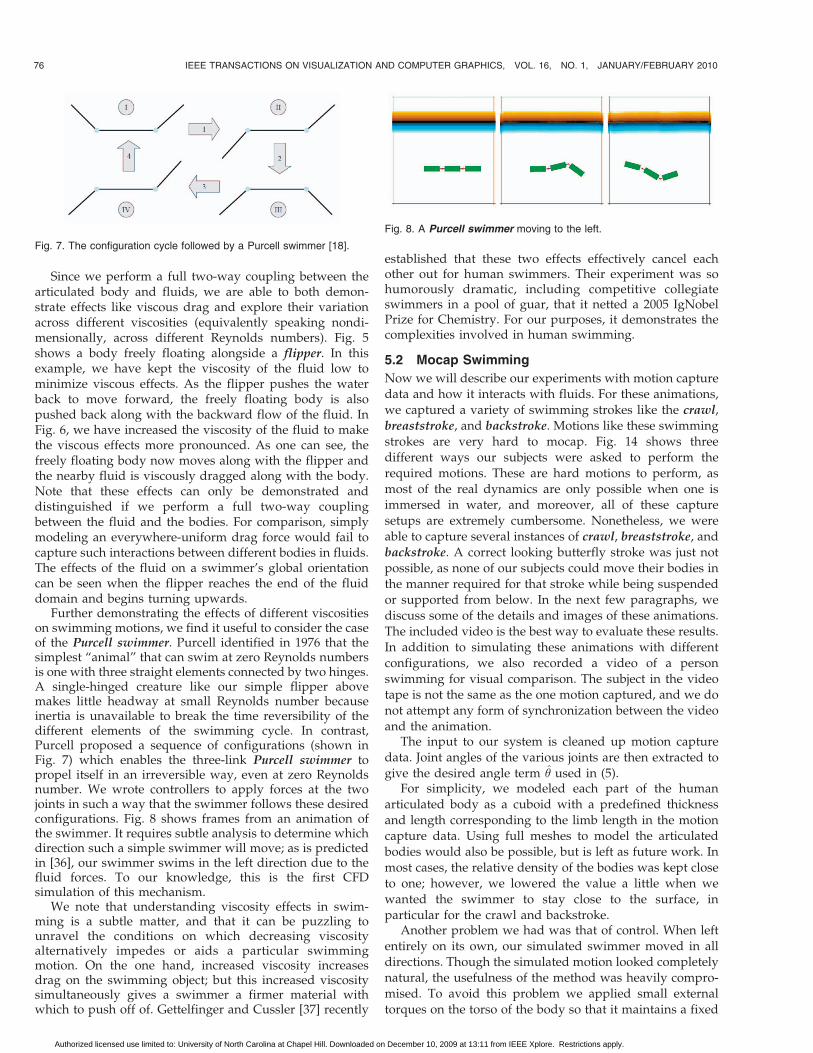
Further demonstrating the effects of different viscositieson swimming motions, we find it useful to consider the caseof the Purcell swimmer. Purcell identified in 1976 that thesimplest “animal” that can swim at zero Reynolds numbersis one with three straight elements connected by two hinges.A single-hinged creature like our simple flipper abovemakes little headway at small Reynolds number becauseinertia is unavailable to break the time reversibility of thedifferent elements of the swimming cycle. In contrast,Purcell proposed a sequence of configurations (shown inFig. 7) which enables the three-link Purcell swimmer topropel itself in an irreversible way, even at zero Reynoldsnumber. We wrote controllers to apply forces at the twojoints in such a way that the swimmer follows these desiredconfigurations. Fig. 8 shows frames from an animation ofthe swimmer. It requires subtle analysis to determine whichdirection such a simple swimmer will move; as is predictedin [36], our swimmer swims in the left direction due to thefluid forces. To our knowledge, this is the first CFDsimulation of this mechanism.

We note that understanding viscosity effects in swim-ming is a subtle matter, and that it can be puzzling tounravel the conditions on which decreasing viscosityalternatively impedes or aids a particular swimmingmotion. On the one hand, increased viscosity increasesdrag on the swimming object; but this increased viscositysimultaneously gives a swimmer a firmer material withwhich to push off of. Gettelfinger and Cussler [37] recently

established that these two effects effectively cancel eachother out for human swimmers. Their experiment was sohumorously dramatic, including competitive collegiateswimmers in a pool of guar, that it netted a 2005 IgNobelPrize for Chemistry. For our purposes, it demonstrates thecomplexities involved in human swimming.

5.2 Mocap Swimming

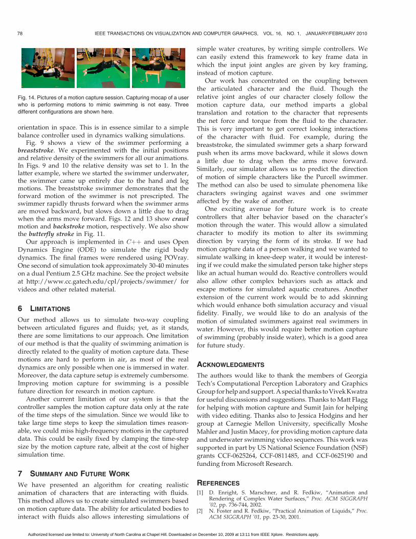
Now we will describe our experiments with motion capturedata and how it interacts with fluids. For these animations,we captured a variety of swimming strokes like the crawl,breaststroke, and backstroke. Motions like these swimmingstrokes are very hard to mocap. Fig. 14 shows threedifferent ways our subjects were asked to perform therequired motions. These are hard motions to perform, asmost of the real dynamics are only possible when one isimmersed in water, and moreover, all of these capturesetups are extremely cumbersome. Nonetheless, we wereable to capture several instances of crawl, breaststroke, andbackstroke. A correct looking butterfly stroke was just notpossible, as none of our subjects could move their bodies inthe manner required for that stroke while being suspendedor supported from below. In the next few paragraphs, wediscuss some of the details and images of these animations.The included video is the best way to evaluate these results.In addition to simulating these animations with differentconfigurations, we also recorded a video of a personswimming for visual comparison. The subject in the videotape is not the same as the one motion captured, and we donot attempt any form of synchronization between the videoand the animation.

The input to our system is cleaned up motion capturedata. Joint angles of the various joints are then extracted togive the desired angle term � used in (5).

For simplicity, we modeled each part of the humanarticulated body as a cuboid with a predefined thicknessand length corresponding to the limb length in the motioncapture data. Using full meshes to model the articulatedbodies would also be possible, but is left as future work. Inmost cases, the relative density of the bodies was kept closeto one; however, we lowered the value a little when wewanted the swimmer to stay close to the surface, inparticular for the crawl and backstroke.

Another problem we had was that of control. When leftentirely on its own, our simulated swimmer moved in alldirections. Though the simulated motion looked completelynatural, the usefulness of the method was heavily compro-mised. To avoid this problem we applied small externaltorques on the torso of the body so that it maintains a fixed


Fig. 7. The configuration cycle followed by a Purcell swimmer [18].

Fig. 8. A Purcell swimmer moving to the left.



Fig. 9. Breaststroke.

Fig. 10. Underwater breaststroke.

Fig. 11. Butterfly.

Fig. 12. Crawl.

Fig. 13. Backstroke.


orientation in space. This is in essence similar to a simplebalance controller used in dynamics walking simulations.

Fig. 9 shows a view of the swimmer performing abreaststroke. We experimented with the initial positionsand relative density of the swimmers for all our animations.In Figs. 9 and 10 the relative density was set to 1. In thelatter example, where we started the swimmer underwater,the swimmer came up entirely due to the hand and legmotions. The breaststroke swimmer demonstrates that theforward motion of the swimmer is not prescripted. Theswimmer rapidly thrusts forward when the swimmer armsare moved backward, but slows down a little due to dragwhen the arms move forward. Figs. 12 and 13 show crawlmotion and backstroke motion, respectively. We also showthe butterfly stroke in Fig. 11.

Our approach is implemented in Cþþ and uses OpenDynamics Engine (ODE) to simulate the rigid bodydynamics. The final frames were rendered using POVray.One second of simulation took approximately 30-40 minuteson a dual Pentium 2.5 GHz machine. See the project websiteat http://www.cc.gatech.edu/cpl/projects/swimmer/ forvideos and other related material.

6 LIMITATIONS

Our method allows us to simulate two-way couplingbetween articulated figures and fluids; yet, as it stands,there are some limitations to our approach. One limitationof our method is that the quality of swimming animation isdirectly related to the quality of motion capture data. Thesemotions are hard to perform in air, as most of the realdynamics are only possible when one is immersed in water.Moreover, the data capture setup is extremely cumbersome.Improving motion capture for swimming is a possiblefuture direction for research in motion capture.

Another current limitation of our system is that thecontroller samples the motion capture data only at the rateof the time steps of the simulation. Since we would like totake large time steps to keep the simulation times reason-able, we could miss high-frequency motions in the captureddata. This could be easily fixed by clamping the time-stepsize by the motion capture rate, albeit at the cost of highersimulation time.

7 SUMMARY AND FUTURE WORK

We have presented an algorithm for creating realisticanimation of characters that are interacting with fluids.This method allows us to create simulated swimmers basedon motion capture data. The ability for articulated bodies tointeract with fluids also allows interesting simulations of

simple water creatures, by writing simple controllers. Wecan easily extend this framework to key frame data inwhich the input joint angles are given by key framing,instead of motion capture.

Our work has concentrated on the coupling betweenthe articulated character and the fluid. Though therelative joint angles of our character closely follow themotion capture data, our method imparts a globaltranslation and rotation to the character that representsthe net force and torque from the fluid to the character.This is very important to get correct looking interactionsof the character with fluid. For example, during thebreaststroke, the simulated swimmer gets a sharp forwardpush when its arms move backward, while it slows downa little due to drag when the arms move forward.Similarly, our simulator allows us to predict the directionof motion of simple characters like the Purcell swimmer.The method can also be used to simulate phenomena likecharacters swinging against waves and one swimmeraffected by the wake of another.

One exciting avenue for future work is to createcontrollers that alter behavior based on the character’smotion through the water. This would allow a simulatedcharacter to modify its motion to alter its swimmingdirection by varying the form of its stroke. If we hadmotion capture data of a person walking and we wanted tosimulate walking in knee-deep water, it would be interest-ing if we could make the simulated person take higher stepslike an actual human would do. Reactive controllers wouldalso allow other complex behaviors such as attack andescape motions for simulated aquatic creatures. Anotherextension of the current work would be to add skinningwhich would enhance both simulation accuracy and visualfidelity. Finally, we would like to do an analysis of themotion of simulated swimmers against real swimmers inwater. However, this would require better motion captureof swimming (probably inside water), which is a good areafor future study.

ACKNOWLEDGMENTS

The authors would like to thank the members of GeorgiaTech’s Computational Perception Laboratory and GraphicsGroup for help and support. A special thanks to Vivek Kwatrafor useful discussions and suggestions. Thanks to Matt Flaggfor helping with motion capture and Sumit Jain for helpingwith video editing. Thanks also to Jessica Hodgins and hergroup at Carnegie Mellon University, specifically MosheMahler and Justin Macey, for providing motion capture dataand underwater swimming video sequences. This work wassupported in part by US National Science Foundation (NSF)grants CCF-0625264, CCF-0811485, and CCF-0625190 andfunding from Microsoft Research.

REFERENCES

[1] D. Enright, S. Marschner, and R. Fedkiw, “Animation andRendering of Complex Water Surfaces,” Proc. ACM SIGGRAPH’02, pp. 736-744, 2002.

[2] N. Foster and R. Fedkiw, “Practical Animation of Liquids,” Proc.ACM SIGGRAPH ’01, pp. 23-30, 2001.


Fig. 14. Pictures of a motion capture session. Capturing mocap of a user

who is performing motions to mimic swimming is not easy. Three

different configurations are shown here.


[3] A. Robinson-Mosher, T. Shinar, J. Gretarsson, J. Su, and R. Fedkiw,“Two-Way Coupling of Fluids to Rigid and Deformable Solidsand Shells,” Proc. ACM SIGGRAPH ’08, pp. 1-9, 2008.

[4] R. Bridson and M. Muller-Fischer, “Fluid Simulation: Siggraph2007 Course Notes,” Proc. ACM SIGGRAPH ’07, pp. 1-81, 2007.

[5] A. Bruderlin and L. Williams, “Motion Signal Processing,” Proc.ACM SIGGRAPH ’95, pp. 97-104, 1995.

[6] M. Gleicher, “Retargetting Motion to New Characters,” Proc. ACMSIGGRAPH ’98, pp. 33-42, 1998.

[7] L. Kovar, M. Gleicher, and F. Pighin, “Motion Graphs,” Proc. ACMSIGGRAPH ’02, pp. 473-482, 2002.

[8] J. Lee, J. Chai, P.S.A. Reitsma, J.K. Hodgins, and N.S. Pollard,“Interactive Control of Avatars Animated with Human MotionData,” Proc. ACM SIGGRAPH ’02, pp. 491-500, 2002.

[9] M. Carlson, P.J. Mucha, and G. Turk, “Rigid Fluid: Animating theInterplay between Rigid Bodies and Fluid,” ACM Trans. Graphics,vol. 23, no. 3, pp. 377-384, 2004.

[10] J.F. O’Brien, V.B. Zordan, and J.K. Hodgins, “CombiningActive and Passive Simulations for Secondary Motion,” IEEEComputer Graphics & Applications, vol. 20, no. 4, pp. 86-96,July/Aug. 2000.

[11] N. Foster and D. Metaxas, “Realistic Animation of Liquids,”Graphical Models and Image Processing, vol. 58, no. 5, pp. 471-483,1996.

[12] O. Genevaux, A. Habibi, and J.-M. Dischler, “SimulatingFluid-Solid Interaction,” Proc. Graphics Interface, pp. 31-38, June2003.

[13] E. Guendelman, A. Selle, F. Losasso, and R. Fedkiw, “CouplingWater and Smoke to Thin Deformable and Rigid Shells,” ACMTrans. Graphics, vol. 24, no. 3, pp. 973-981, 2005.

[14] F. Losasso, G. Irving, E. Guendelman, and R. Fedkiw, “Meltingand Burning Solids into Liquids and Gases,” IEEE Trans.Visualization and Computer Graphics, vol. 12, no. 3, pp. 343-352,May/June 2006.

[15] B.M. Klingner, B.E. Feldman, N. Chentanez, and J.F. O’Brien,“Fluid Animation with Dynamic Meshes,” ACM Trans. Graphics,vol. 25, no. 3, pp. 820-825, Aug. 2006.

[16] N. Chentanez, T.G. Goktekin, B. Feldman, and J. O’Brien,“Simultaneous Coupling of Fluids and Deformable Bodies,” Proc.ACM SIGGRAPH/Eurographics Symp. Computer Animation (SCA’06), pp. 325-333, 2006.

[17] C. Batty, F. Bertails, and R. Bridson, “A Fast Variational Frame-work for Accurate Solid-Fluid Coupling,” ACM Trans. Graphics,vol. 26, no. 3, p. 100, 2007.

[18] E. Purcell, “Life at Low Reynolds Number,” Am. J. Physics, vol. 45,pp. 3-11, 1976.

[19] M. Oshita and A. Makinouchi, “A Dynamic Motion ControlTechnique for Human-Like Articulated Figures,” Computer Gra-phics Forum, vol. 20, no. 3, 2001.

[20] V.B. Zordan and J.K. Hodgins, “Motion Capture-Driven Simula-tions that Hit and React,” Proc. ACM SIGGRAPH/EurographicsSymp. Computer Animation (SCA ’02), pp. 89-96, 2002.

[21] P.-F. Yang, J. Laszlo, and K. Singh, “Layered Dynamic Control forInteractive Character Swimming,” Proc. ACM SIGGRAPH/Euro-graphics Symp. Computer Animation (SCA ’04), pp. 39-47, 2004.

[22] M.A. MacIver, N.A. Patankar, B. Gooch, V. Oza, S. Lee, and O.Curet, “Numerical Simulation of Freely Swimming Fish,”J. Computational Physics, vol. 228, no. 7, pp. 2366-2390, 2009.

[23] X. Tu and D. Terzopoulos, “Artificial Fishes: Physics, Locomotion,Perception, Behavior,” Proc. ACM SIGGRAPH ’94, pp. 43-50, 1994.

[24] J.-C. Wu and Z. Popovic, “Realistic Modeling of Bird FlightAnimations,” ACM Trans. Graphics, vol. 22, no. 3, pp. 888-895,2003.

[25] G.D. Yngve, J.F. O’Brien, and J.K. Hodgins, “Animating Explo-sions,” Proc. ACM SIGGRAPH ’00, pp. 29-36, 2000.

[26] T. Takahashi, U. Heihachi, and A. Kunimatsu, “The Simulation ofFluid-Rigid Body Interaction,” Proc. ACM SIGGRAPH ’02, p. 266,2002.

[27] T. Takahashi, H. Fujii, A. Kunimatsu, K. Hiwada, T. Saito, K.Tanaka, and H. Ueki, “Realistic Animation of Fluid with Splashand Foam,” Computer Graphics Forum, vol. 22, no. 3, pp. 391-400,2003.

[28] J.K. Hodgins, W.L. Wooten, D.C. Brogan, and J.F. O’Brien,“Animating Human Athletics,” Proc. ACM SIGGRAPH ’95,pp. 71-78, 1995.

[29] P. Faloutsos, M. van de Panne, and D. Terzopoulos, “Compo-sable Controllers for Physics-Based Character Animation,” Proc.ACM SIGGRAPH ’01, pp. 251-260, 2001.

[30] S. Redon, N. Galoppo, and M.C. Lin, “Adaptive Dynamics ofArticulated Bodies,” ACM Trans. Graphics, vol. 24, no. 3, pp. 936-945, 2005.

[31] R. Featherstone, Robot Dynamics Algorithm. Kluwer AcademicPublishers, 1987.

[32] D. Halliday and R. Resnick, Physics: Parts I and II. Wiley, 1978.[33] K. Shoemaker, “Animating Rotation with Quaternion Curves,”

Proc. ACM SIGGRAPH ’85, pp. 245-254, 1985.[34] J. Stam, “Stable Fluids,” Proc. ACM SIGGRAPH ’99, pp. 121-128,

1999.[35] B. Kim, Y. Liu, I. Llamas, and J. Rossignac, “Flowfixer: Using Bfecc

for Fluid Simulation,” Proc. Eurographics Workshop NaturalPhenomena, 2005.

[36] L.E. Becker, S.A. Koehler, and H.A. Stone, “On Self-Propulsion ofMicro-Machines at Low Reynolds Number: Purcell’s Three-LinkSwimmer,” J. Fluid Mechanics, vol. 490, pp. 15-35, 2003.

[37] B. Gettelfinger and E.L. Cussler, “Will Humans Swim Faster orSlower in Syrup?” Am. Inst. of Chemical Eng. J., vol. 50, pp. 2646-2647, 2004.

Nipun Kwatra received the BTech degree incomputer science from the Indian Institute ofTechnology, Delhi, in 2004 and the MS degreefrom Georgia Institute of Technology in 2006. Heis a PhD candidate at Stanford University, underthe guidance of Professor Ronald Fedkiw. Hisresearch is focused on computer graphics andcomputational physics, particularly physicallybased simulation of natural phenomena.

Chris Wojtan received the BS degree incomputer science from the University of Illinoisin Urbana-Champaign in 2004 and received aNational Science Foundation Graduate Fellow-ship in 2005. He is a PhD student in the College ofComputing at the Georgia Institute of Technol-ogy. His interests include physics-based anima-tion, numerical methods, and applied geometry.

Mark Carlson received the BS degree incomputer science, with a minor in creativewriting, from the University of Central Florida in1997, and earned the PhD degree in computerscience, with a minor in computational physics,from Georgia Institute of Technology, in 2004. Hewrote a fluid simulator for DNA Productionswhere he also worked as a visual effects artistfor the movie “Ant Bully.” He was a seniorsoftware developer at Walt Disney Animation

Studios, and is currently in the FX R&D group at DreamWorks Animation.



Irfan Essa received the MS degree in 1990 andthe PhD degree in 1994. He also held a researchfaculty position at the Massachusetts Institute ofTechnology (Media Lab) (1988-1996). In 1996,he joined the Georgia Institute of TechnologyFaculty. He is a professor in the School ofInteractive Computing (SIC) of the College ofComputing (CoC) at the Georgia Institute ofTechnology, in Atlanta. At Georgia Tech, he isprimarily affiliated with two interdepartmental

centers: the Robotics & Machine Intelligence (RIM@GT) Center andthe GVU Center. He works in the areas of computer vision, computergraphics, computational perception, robotics and computer animation,with potential impact on video analysis and production (e.g., computa-tional photography, image-based modeling and rendering, etc.), humancomputer interaction, and artificial intelligence research. He haspublished more than 150 scholarly articles in leading journals andconference venues on these topics. He has been awarded the USNational Science Foundation (NSF) CAREER Award and within GATech, he has won the College of Computings Junior and SeniorResearch Faculty Awards, Outstanding Teacher Award, InstitutesEducational Innovation Award, and the Deans Award. He is a seniormember of the IEEE and the IEEE Computer Society.

Peter J. Mucha received the PhD degree inapplied and computational mathematics in 1998from Princeton University. He was an appliedmathematics instructor at the MassachusettsInstitute of Technology (MIT) for three years,followed by four years as an assistant professorin mathematics at the Georgia Institute ofTechnology. He is currently an associate pro-fessor at the University of North Carolina atChapel Hill, where he is a member of the

Department of Mathematics and the Institute for Advanced Materials,Nanoscience, and Technology.

Greg Turk received the PhD degree in computerscience in 1992 from the University of NorthCarolina at Chapel Hill (UNC Chapel Hill). Hewas a postdoctoral researcher at StanfordUniversity for two years, followed by two yearsas a research scientist at UNC Chapel Hill. He iscurrently a professor at the Georgia Institute ofTechnology, where he is a member of theSchool of Interactive Computing and the Gra-phics, Visualization, and Usability Center. His

research interests include computer graphics, scientific visualization,and computer vision. In 2008, he was the technical papers chair for ACMSIGGRAPH. He is a member of the IEEE.

. For more information on this or any other computing topic,please visit our Digital Library at www.computer.org/publications/dlib.



Date post:	29-Jul-2018
Category:	Documents
Upload:	ledat
View:	217 times
Download:	0 times

70 IEEE TRANSACTIONS ON VISUALIZATION AND COMPUTER ...mucha/Reprints/TVCGswimming.pdf · HE field...

Documents