7.1 - 1 Copyright © 2010, 2007, 2004 Pearson Education, Inc. All Rights Reserved. Chapter 7...

7.1 - 1Copyright © 2010, 2007, 2004 Pearson Education, Inc. All Rights Reserved.

Chapter 7Estimates and Sample Sizes

7-1 Review and Preview

7-2 Estimating a Population Proportion

7-3 Estimating a Population Mean: σ Known (OMIT)

7-4 Estimating a Population Mean: σ Not Known

7-5 Estimating a Population Variance (OMIT)


Section 7-1Review and Preview


Review

Chapters 2 & 3 we used “descriptive statistics” when we summarized data using tools such as graphs, and statistics such as the mean and standard deviation.

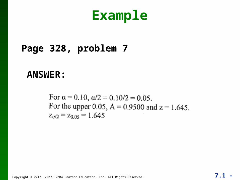
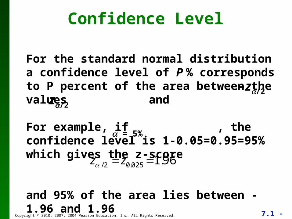
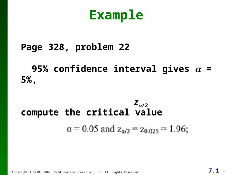
Chapter 6 we introduced critical values:z denotes the z score with an area of to its right.If = 0.025, the critical value is z0.025 = 1.96.That is, the critical value z0.025 = 1.96 has an area of 0.025 to its right.


Preview

The two major activities of inferential statistics are (1) to use sample data to estimate values of a population parameters, and (2) to test hypotheses or claims made about population parameters.

We introduce methods for estimating values of these important population parameters: proportions, means, and variances.

We also present methods for determining sample sizes necessary to estimate those parameters.

This chapter presents the beginning of inferential statistics.


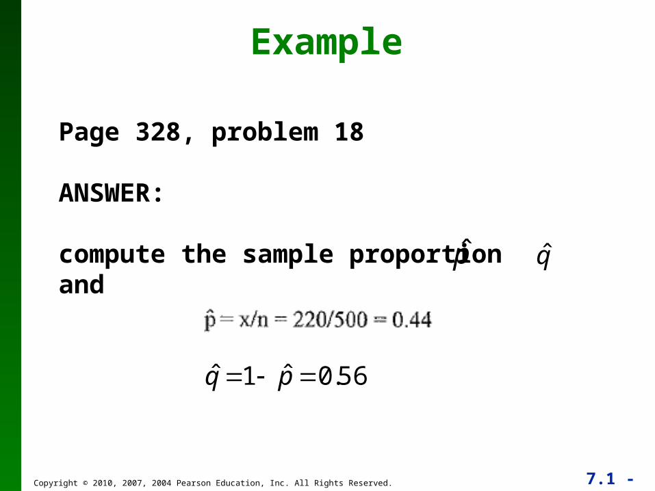
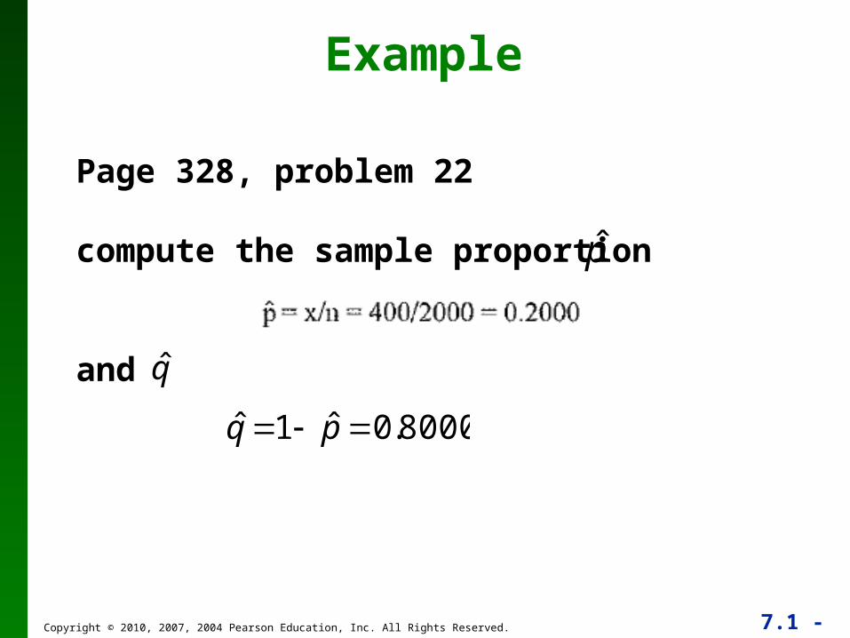
Section 7-2 Estimating a Population

Proportion


Key ConceptIn this section we present methods for using a sample proportion to estimate the value of a population proportion.

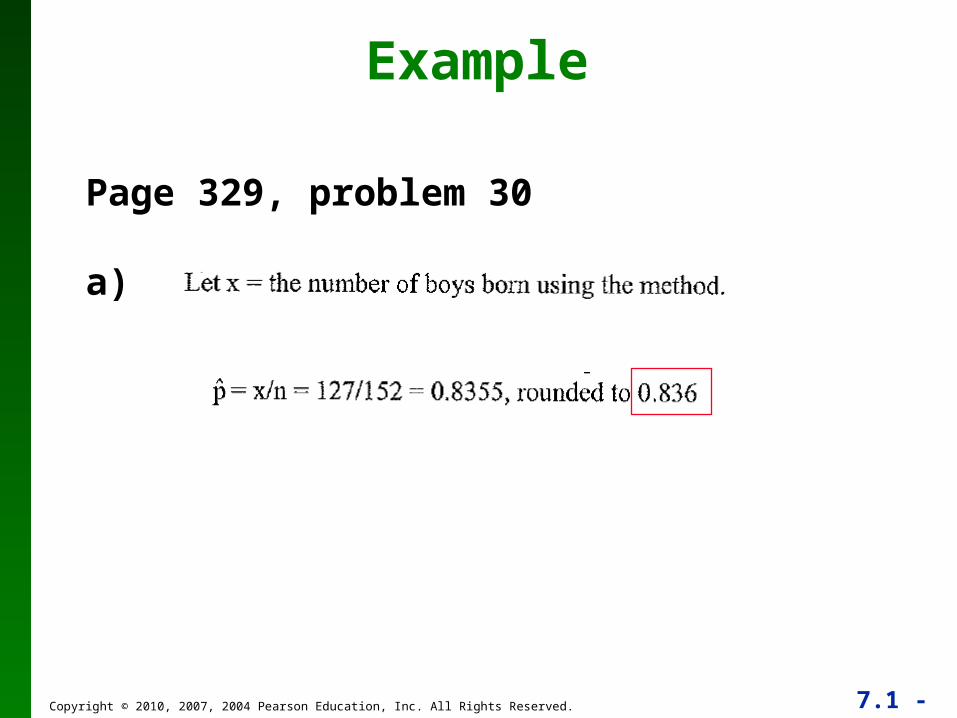
• The sample proportion is the best point estimate of the population proportion.

• We can use a sample proportion to construct a confidence interval to estimate the true value of a population proportion, and we should know how to interpret such confidence intervals.

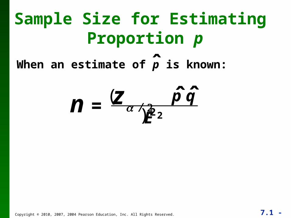
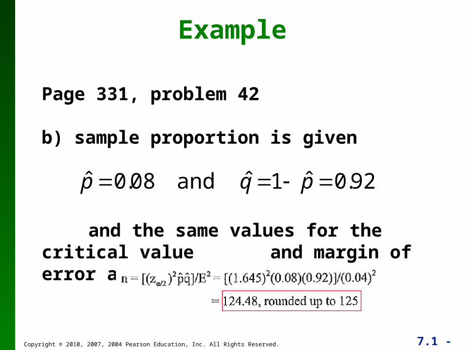
• We should know how to find the sample size necessary to estimate a population proportion.


Definition

A point estimate is a single value (or point) used to approximate a population parameter.


The sample proportion p is the best point estimate of the population proportion p.

ˆ

Definition


Example:

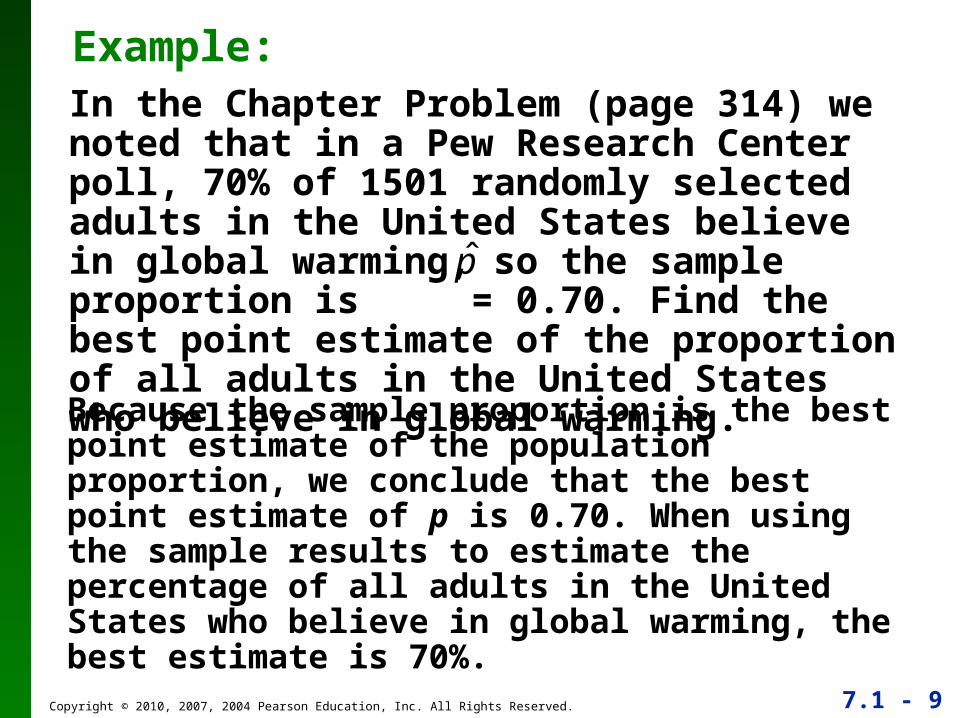
Because the sample proportion is the best point estimate of the population proportion, we conclude that the best point estimate of p is 0.70. When using the sample results to estimate the percentage of all adults in the United States who believe in global warming, the best estimate is 70%.

In the Chapter Problem (page 314) we noted that in a Pew Research Center poll, 70% of 1501 randomly selected adults in the United States believe in global warming, so the sample proportion is = 0.70. Find the best point estimate of the proportion of all adults in the United States who believe in global warming.

p̂


Definition

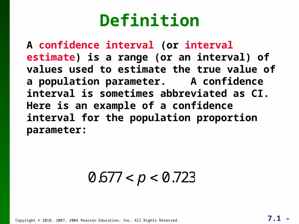
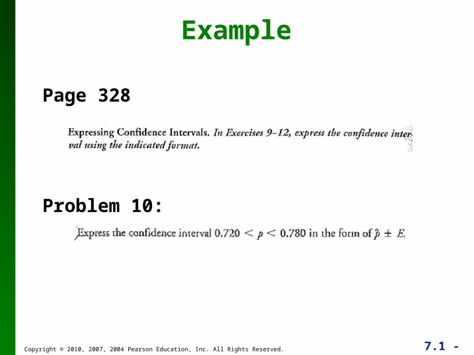
A confidence interval (or interval estimate) is a range (or an interval) of values used to estimate the true value of a population parameter. A confidence interval is sometimes abbreviated as CI. Here is an example of a confidence interval for the population proportion parameter:

0.677 p 0.723


NOTE

We will learn how to construct confidence intervals from a sample statistic later using a formula.


We must be careful to interpret confidence intervals correctly. There is a correct interpretation and many different and creative incorrect interpretations of the confidence interval a < p < b

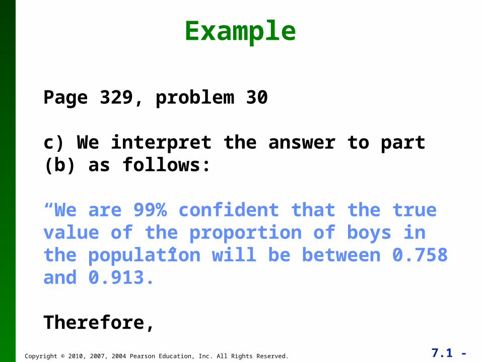
Typically, we interpret the 95% confidence interval as follows:“We are 95% confident that the interval from a to b actually does contain the true value of the population proportion p.”

Interpreting a Confidence Interval


This means that if we were to select many different samples of the same size and construct the corresponding confidence intervals, 95% of them would actually contain the value of the population proportion p.(Note that in this correct interpretation, the level of 95% refers to the success rate of the process being used to estimate the proportion.)



For example, if we calculate the 95% confidence intervals for 20 different samples of a population, we expect that 95% of the 20 samples, or 19 samples, would have confidence intervals that contain the true value of p.



Consider the chapter problem example (global warming) again. Suppose we know the true proportion of all adults who believe in global warming is p=0.75With 95% confidence interval, if we sample 20 times we may compute a confidence interval which does not actually contain p=0.75, such as,

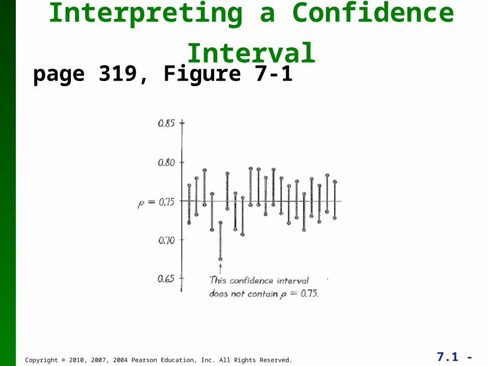
but, 19 times out of 20 we would find confidence intervals that do contain p=0.75.This is illustrated in Figure 7-1.


0.677 p 0.723


page 319, Figure 7-1



Know the correct interpretation of a confidence interval.

Caution


NEXT

We will learn now discuss how to construct confidence intervals from a sample statistic.


Critical ValuesA standard z score can be used to distinguish between sample statistics that are likely to occur and those that are unlikely to occur. Such a z score is called a critical value. Critical values are based on the following observations:

Under certain conditions, the sampling distribution of sample proportions can be approximated by a normal distribution.


Critical ValuesDEFINE: A z score of associated with a sample proportion has a probability of /2 of falling in the right tail. Therefore:

2/z

To find , find the z-score in Table A-2 that corresponds to an area of

2/z

2/1


Example

Page 328, problem 7

Find z/2 for =0.10


Example

Page 328, problem 7

ANSWER:


Definition

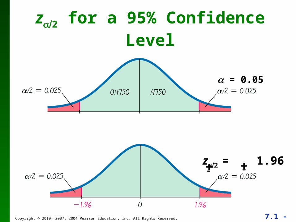
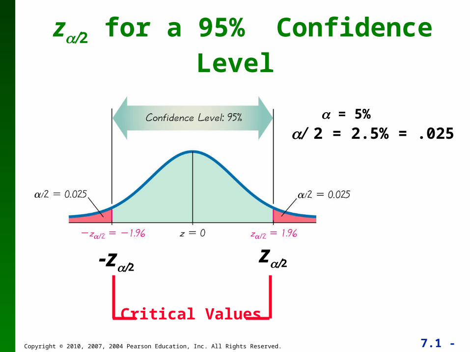
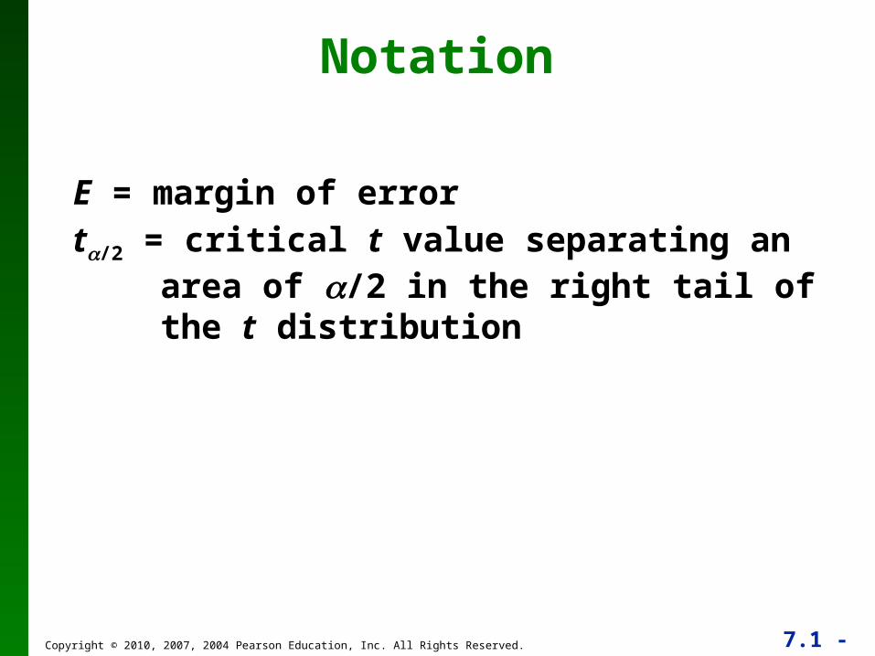
A critical value is the number on the borderline separating sample statistics that are likely to occur from those that are unlikely to occur. The number z/2 is a critical value that is a z score with the property that it separates an area of /2 in the right tail of the standard normal distribution.


Critical Value

Because the standard normal distribution is symmetric about the value of z=0, the value of –z/2 is at the vertical boundary for the area of /2 in the left tail


The Critical Value z2

-z/2


A confidence level is the probability 1 – (often expressed as the equivalent percentage value) that the confidence interval actually does contain the population parameter, assuming that the estimation process is repeated a large number of times. (The confidence level is also called degree of confidence, or the confidence coefficient.)

Definition


Common choices for confidence levels are:

90% confidence level where = 10%,



Definition


Confidence Level

For the standard normal distribution a confidence level of P % corresponds to P percent of the area between the values and

For example, if , the confidence level is 1-0.05=0.95=95% which gives the z-score

and 95% of the area lies between -1.96 and 1.96

–z/2

z/2

= 5%

96.1025.02/ zz


z2 = 1.96

= 0.05

z2 for a 95% Confidence Level


z2 for a 95% Confidence Level

-z2z2

Critical Values

2 = 2.5% = .025 = 5%


Definition

When data from a simple random sample are used to

estimate a population proportion p, the margin of

error, denoted by E, is the maximum likely difference

(with probability 1 – , such as 0.95) between the

observed proportion and the true value of the

population proportion p. The margin of error E is

also called the maximum error of the estimate and

can be found by multiplying the critical value and

the standard deviation of the sample proportions:

p̂


Margin of Error for Proportions

2

ˆ ˆpqE z

n

pq ˆ1ˆ NOTE:


p = population proportion

Confidence Interval for Estimating a Population Proportion p

= sample proportion

n = number of sample values

E = margin of error

z/2 = z score separating an area of /2 in the right tail of the standard normal distribution

p̂


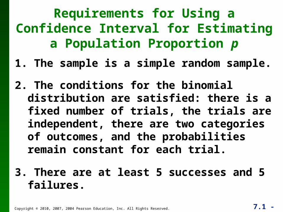
Requirements for Using a Confidence Interval for Estimating a Population

Proportion p

1. The sample is a simple random sample.

2. The conditions for the binomial distribution are satisfied: there is a fixed number of trials, the trials are independent, there are two categories of outcomes, and the probabilities remain constant for each trial.

3. There are at least 5 successes and 5 failures.



p – E < < + Eˆ p ˆ

p

where

2

ˆ ˆpqE z

n


p – E < < + E

p + E

p p ˆ

ˆ


ˆ

(p – E, p + E)ˆ ˆ


Round-Off Rule for Confidence Interval Estimates of p

Round the confidence interval limits for p to

three significant digits.


Example

Page 328

Problem 18:


Example

Page 328, problem 18

ANSWER:

compute the critical value z/2


Example


ANSWER:

compute the sample proportion andp̂

56.0ˆ1ˆ pq

q̂


Example


ANSWER:

compute the margin of error E


Calculator UseHere is what the solution manual suggests

Calculate first

To use the formula on a TI calculator:

Calculate , press the multiply key, the parentheses key, then 1- ANS (ANS is the 2nd (-) key on bottom row) , then ENTER. This will give

z/2

p̂

qp ˆˆ


Example

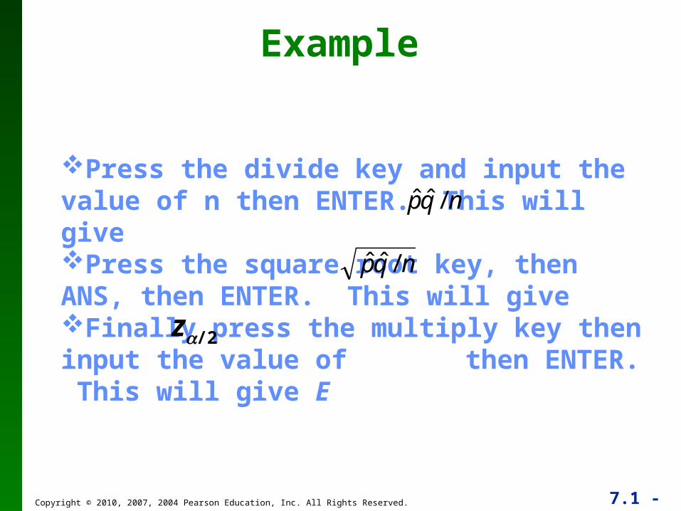
Press the divide key and input the value of n then ENTER. This will give Press the square root key, then ANS, then ENTER. This will give Finally press the multiply key then input the value of then ENTER. This will give Ez/2

nqp /ˆˆ

nqp /ˆˆ


1. Verify that the required assumptions are satisfied. (The sample is a simple random sample, the conditions for the binomial distribution are satisfied, and the normal distribution can be used to approximate the distribution of sample proportions because np 5, and nq 5 are both satisfied.)

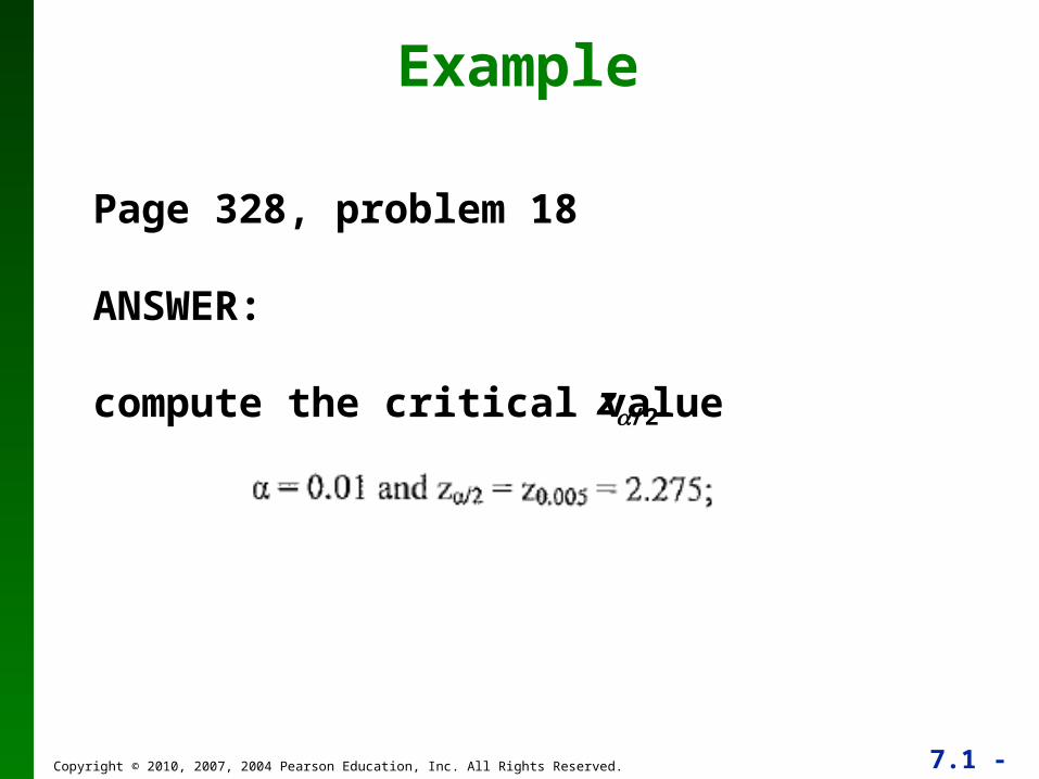
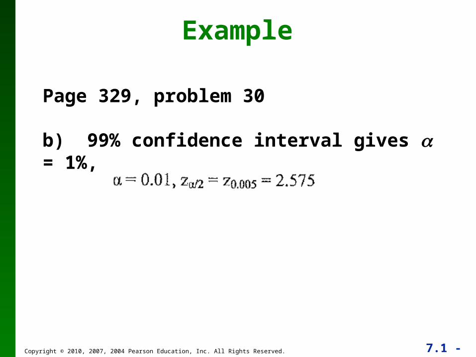
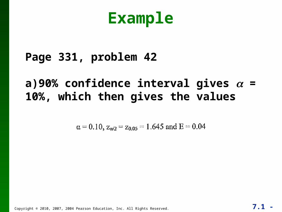
2. Refer to Table A-2 and find the critical value z/2 that corresponds to the desired confidence level.

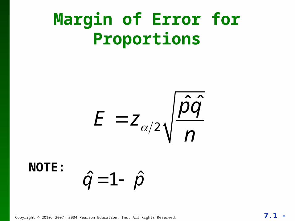
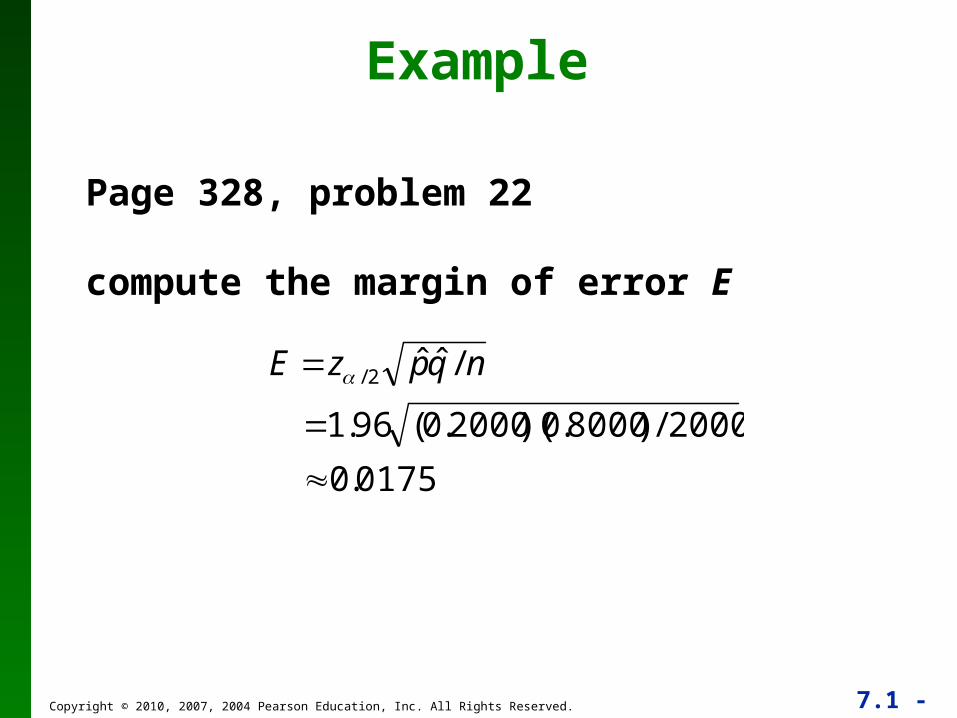
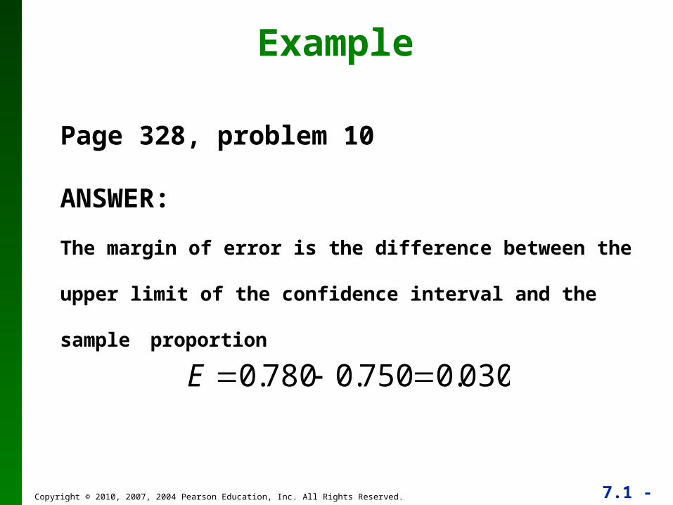
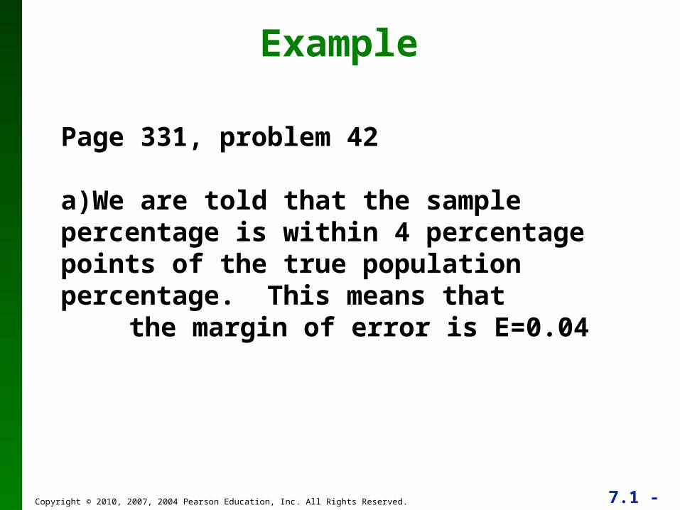
3. Evaluate the margin of error

Procedure for Constructing a Confidence Interval for p

2ˆ Ê z pq n


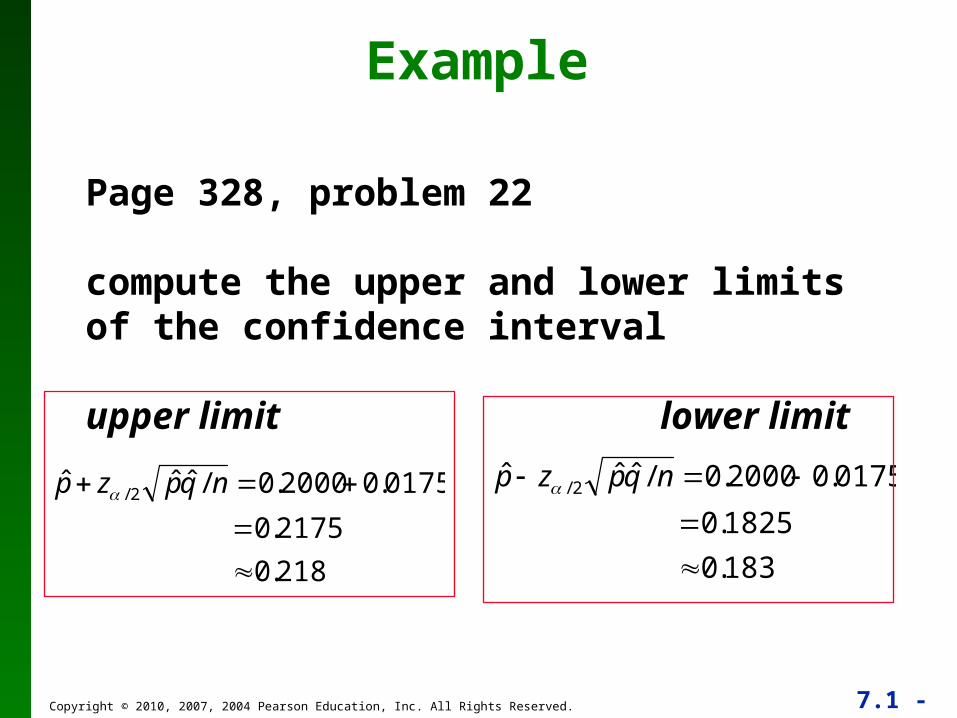
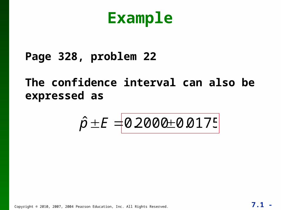
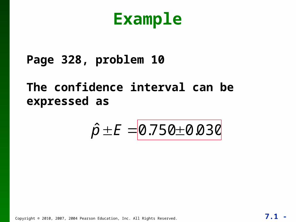
4. Using the value of the calculated margin of error, E and the value of the sample proportion, p, find the values of p – E and p + E. Substitute those values in the general format for the confidence interval:

ˆ

ˆ

ˆ

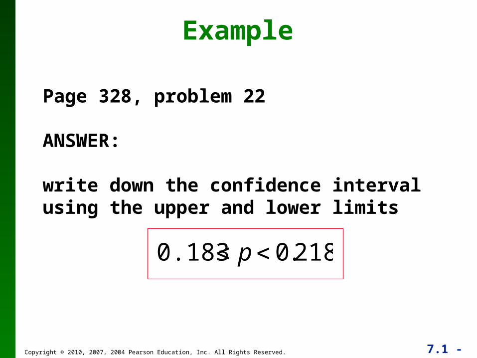
p – E < p < p + E

ˆ

ˆ

5. Round the resulting confidence interval limits to three significant digits.

Procedure for Constructing a Confidence Interval for p - cont


Example

Page 328

Problem 22:


Example


95% confidence interval gives = 5%,

compute the critical value z/2


Example


compute the sample proportion

and

p̂

8000.0ˆ1ˆ pq

q̂


Example


compute the margin of error E

0175.0

2000/)8000.0)(2000.0(96.1

/ˆˆ2/

nqpzE


Example


compute the upper and lower limits of the confidence interval

upper limit lower limit

218.0

2175.0

0175.02000.0/ˆˆˆ 2/

nqpzp

183.0

1825.0

0175.02000.0/ˆˆˆ 2/

nqpzp


Example


ANSWER:

write down the confidence interval using the upper and lower limits

218.00.183 p


Example


The confidence interval can also be expressed as

0175.02000.0ˆ Ep


Example

Page 328

Problem 10:


Example


ANSWER:

The sample proportion is the midpoint of the upper and lower

limits of the confidence interval 750.0

2

780.0720.0ˆ

p


Example


ANSWER:

The margin of error is the difference between the upper limit

of the confidence interval and the sample proportion

030.0750.0780.0 E


Example


The confidence interval can be expressed as

030.0750.0ˆ Ep


Calculate Confidence Intervals Directly From Calculator

The TI calculator will compute confidence intervals as follows:

Press STAT and select TESTSSelect A:1-PropZIntEnter x,n,C-Level and then calculate

You should be able to calculate a confidence interval both ways: use the formula as in previous examples and directly with A:1-PropZInt as above


Example



Example


a)


Example


b) 99% confidence interval gives = 1%,


Example


b) compute the margin of error E

0774.0

152/)1645.0)(8355.0(575.2

/ˆˆ2/

nqpzE


Example


b) compute the upper and lower limits of the confidence interval

upper limit lower limit

913.0

9129.0

0774.08355.0/ˆˆˆ 2/

nqpzp

758.0

7581.0

0774.08355.0/ˆˆˆ 2/

nqpzp


Example


b) ANSWER:

write down the confidence interval using the upper and lower limits

913.00.758 p


Example


c) We interpret the answer to part (b) as follows:

“We are 99% confident that the true value of the proportion of boys in the population will be between 0.758 and 0.913.”

Therefore,


Example


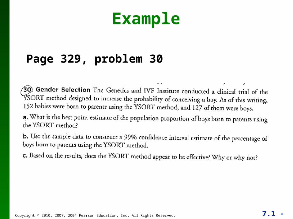
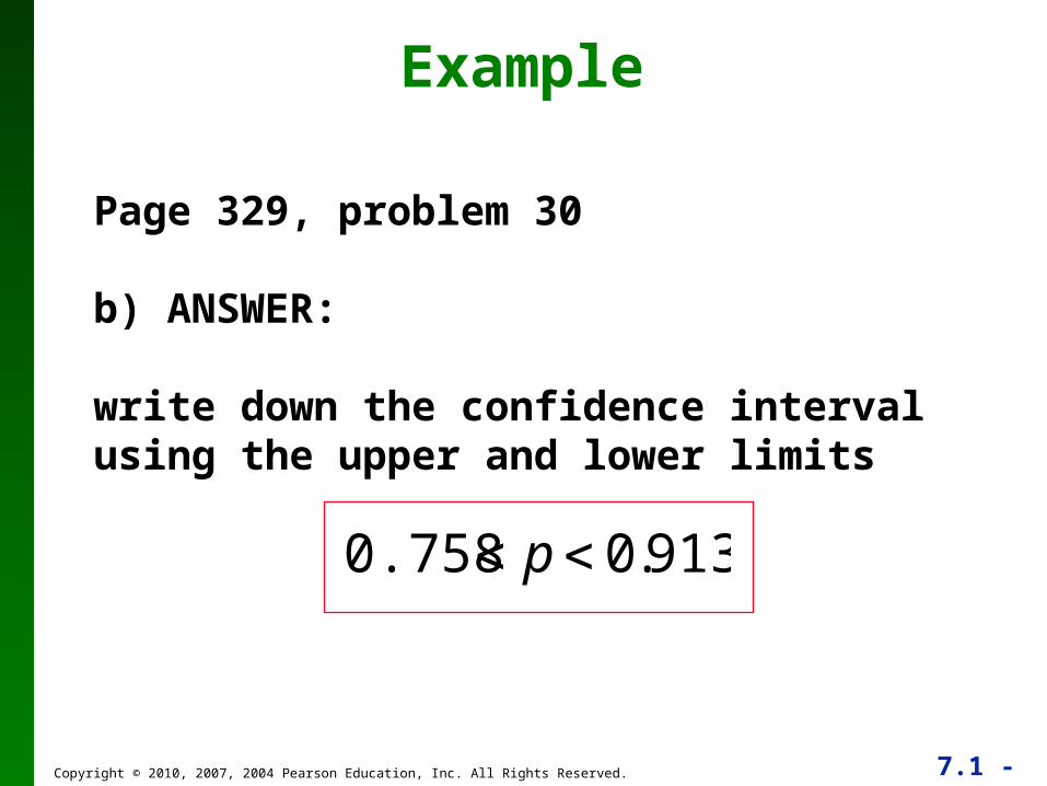
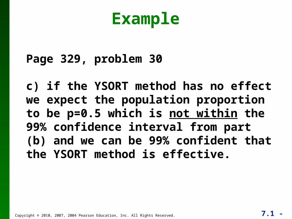
c) if the YSORT method has no effect we expect the population proportion to be p=0.5 which is not within the 99% confidence interval from part (b) and we can be 99% confident that the YSORT method is effective.


Example



Example


a)


Example


b) We interpret the answer to part (a) as follows:

“We are 99% confident that the true value of the proportion of people who say they vote in the population will be between 0.662 and 0.737.”

Therefore,


Example


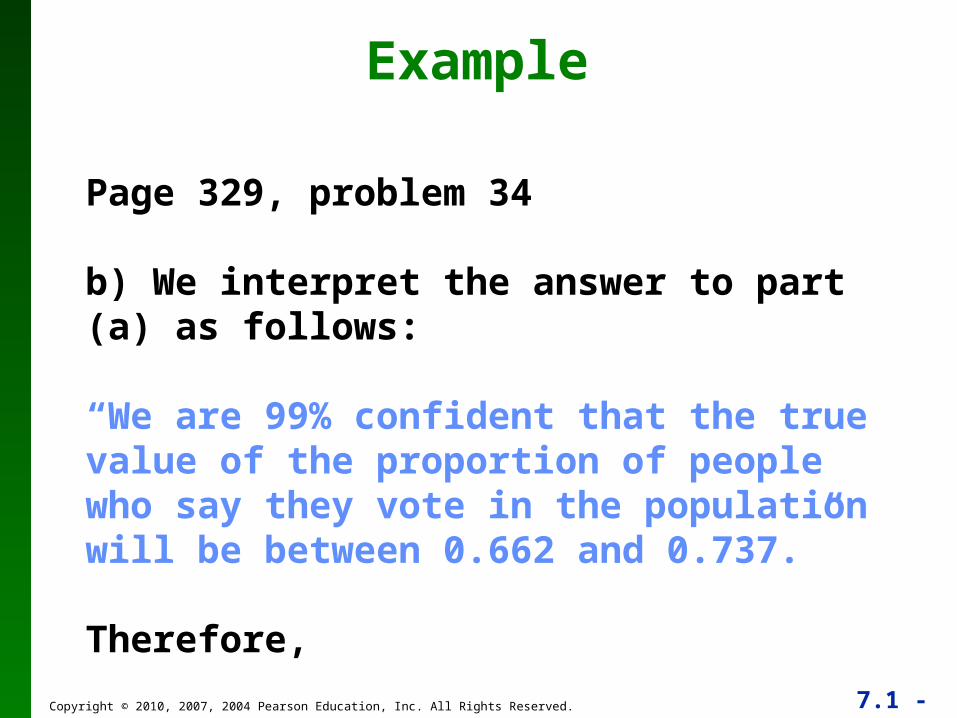
c) since the true population proportion is given as p=0.61 which is not within the 99% confidence interval from part (b), we can be 99% confident that people do not tell the truth about their voting record.


Analyzing PollsWhen analyzing polls consider:

1. The sample should be a simple random sample, not an inappropriate sample (such as a voluntary response sample).

2. The confidence level should be provided. (It is often 95%, but media reports often neglect to identify it.)

3. The sample size should be provided. (It is usually provided by the media, but not always.)

4. Except for relatively rare cases, the quality of the poll results depends on the sampling method and the size of the sample, but the size of the population is usually not a factor.


Caution

Never follow the common misconception that poll results are unreliable if the sample size is a small percentage of the population size. The population size is usually not a factor in determining the reliability of a poll.


Sample Size

Suppose we want to collect sample data in order to estimate some population proportion. The question is how many sample items must be obtained?


Determining Sample Size

(solve for n by algebra)

( )2 ˆp qZ n =

Ê 2

zE =

p qˆ ˆn


Sample Size for Estimating Proportion p

When an estimate of p is known: ˆ

ˆ( )2 p qn =

Ê 2

z


Sample Size for Estimating Proportion p

When no estimate of p is known:

NOTE: here we are assuming that

( )2 0.25n =

E 2

zˆ

50.0ˆˆ qp


Round-Off Rule for Determining Sample Size

If the computed sample size n is not a whole number, round the value of n up to the next larger whole number.


Example



Example


a)We are told that the sample percentage is within 4 percentage points of the true population percentage. This means that

the margin of error is E=0.04


Example


a)90% confidence interval gives = 10%, which then gives the values


Example


a)When sample proportion is unknown use:

to get

50.0ˆˆ qp


Example


b) sample proportion is given

and the same values for the critical value and margin of error as in part (a) to get

92.0ˆ1ˆ and 08.0ˆ pqp


Recap

In this section we have discussed:

Point estimates. Confidence intervals. Confidence levels. Critical values. Margin of error. Determining sample sizes.


Section 7-4 Estimating a Population

Mean: Not Known


Key Concept

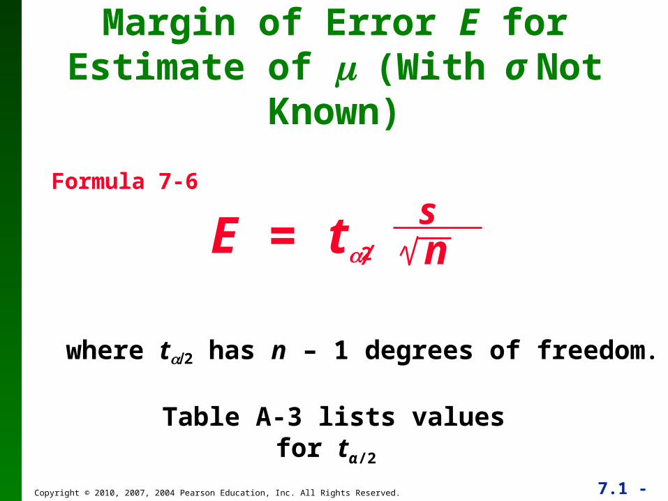
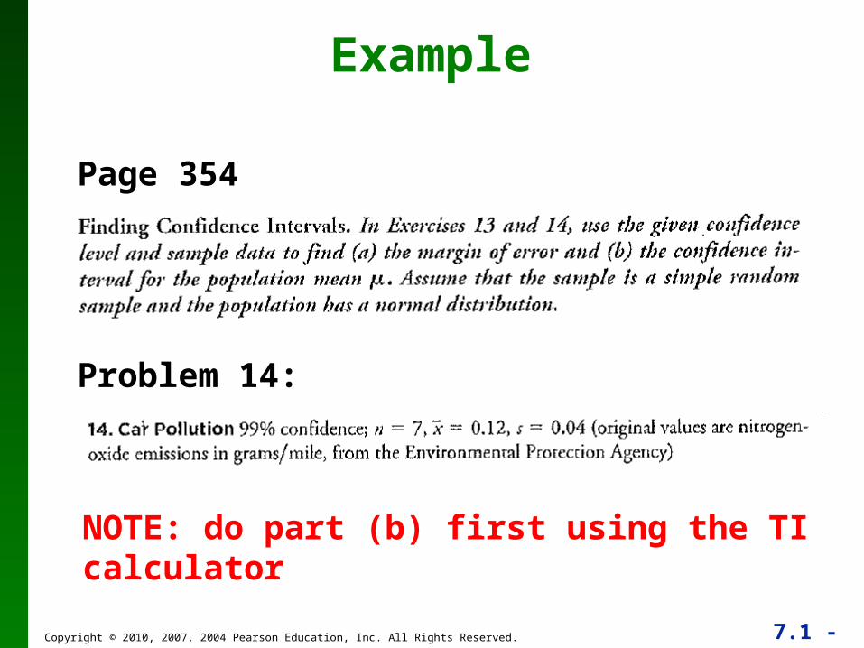
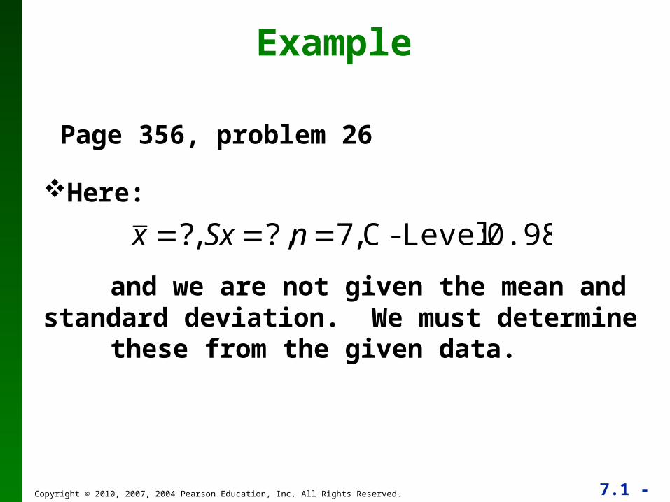
This section presents methods for estimating a population mean when the population standard deviation is not known. With σ unknown, we use the Student t distribution assuming that the relevant requirements are satisfied.


The sample mean is the best point estimate of the population mean.

Sample Mean


= population mean = sample means = sample standard deviationn = number of sample values

Notation

x


If the distribution of a population is essentially normal, then the distribution of

is a Student t Distribution for all samples of size n. It is often referred to as a t distribution and is used to find critical values denoted byt/2.

t =x - µ

sn

Student t Distribution


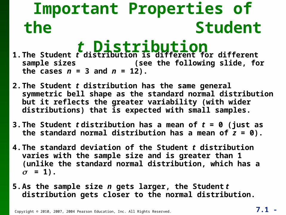
Important Properties of the Student t Distribution

1. The Student t distribution is different for different sample sizes (see the following slide, for the cases n = 3 and n = 12).

2. The Student t distribution has the same general symmetric bell shape as the standard normal distribution but it reflects the greater variability (with wider distributions) that is expected with small samples.

3. The Student t distribution has a mean of t = 0 (just as the standard normal distribution has a mean of z = 0).

4. The standard deviation of the Student t distribution varies with the sample size and is greater than 1 (unlike the standard normal distribution, which has a = 1).

5. As the sample size n gets larger, the Student t distribution gets closer to the normal distribution.


Student t Distributions for n = 3 and n = 12

Figure 7-5


degrees of freedom = n – 1

in this section.

Definition

The number of degrees of freedom for a collection of sample data is the number of sample values that can vary after certain restrictions have been imposed on all data values. The degree of freedom is often abbreviated df.


E = margin of errort/2 = critical t value separating an area of /2

in the right tail of the t distribution

Notation


Margin of Error E for Estimate of (Withσ Not Known)

Formula 7-6

where t2 has n – 1 degrees of freedom.

ns

E = t 2

Table A-3 lists values for tα/2



where E = t/2 ns

x – E < µ < x + E

t/2 found in Table A-3

Confidence Interval for the Estimate of μ (With σ Not Known)

df = n – 1


Example

Use the sample statistics of n = 49, = 0.4 and s = 21.0

to construct a 95% confidence interval estimate of the population mean.

x


With n = 49, the df = 49 – 1 = 48Closest df in Table A-3 is 50, using two tails = 5%=0.05 using one tail /2= 2.5%=0.025

t/2 = 2.009

Example

95% confidence level so

= 5%=0.05


Using t/2 = 2.009, s = 21.0 and n = 49 the margin of error is:

and the confidence interval is

Example

027.649

0.21009.22/

n

stE

x E x E

0.4 6.027 0.4 6.027

5.6 6.4


Requirements for Using a Confidence Interval for Estimating a Population Mean µ

1. The sample is a simple random sample.

2. Either the sample is from a normally distributed population or n>30


2. Using n – 1 degrees of freedom, refer to Table A-3 or use

technology to find the critical value t2 that corresponds to the desired confidence level.

Procedure for Constructing aConfidence Interval for µ

(With σ Unknown)1. Verify that the requirements are satisfied.

3. Evaluate the margin of error E = t2 • s / n .

4. Find the values of Substitute those values in the general format for the confidence interval:

5. Round the resulting confidence interval limits.

x E and x E.

x E x E


Round-Off Rule for Confidence Interval Estimates of µ

If using the original set of data, round to one more decimal place than is used for the original data set.

If using summary statistics ,Sx, n round to the same number of decimal places used for the sample mean

x

x


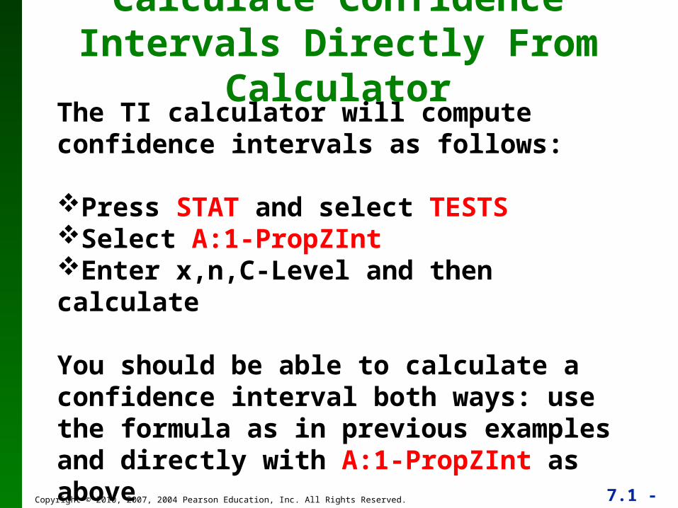
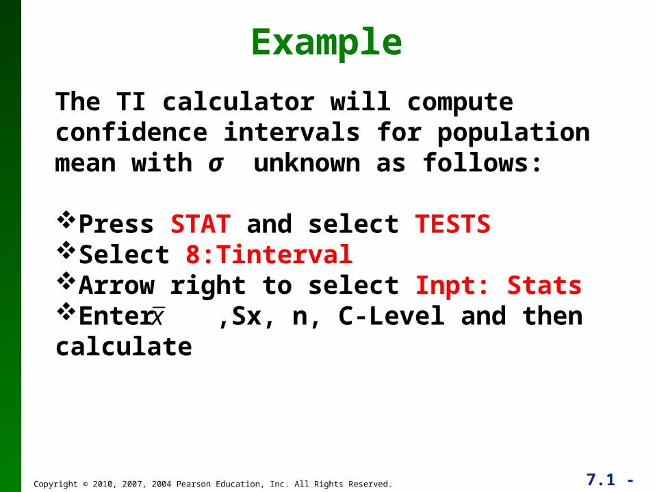
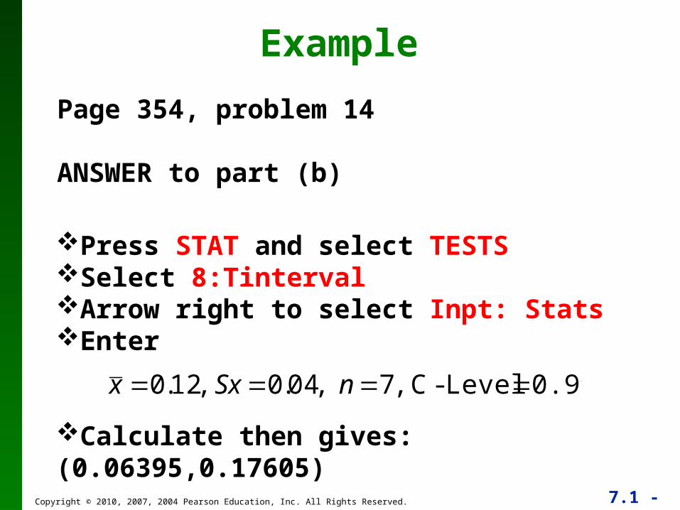
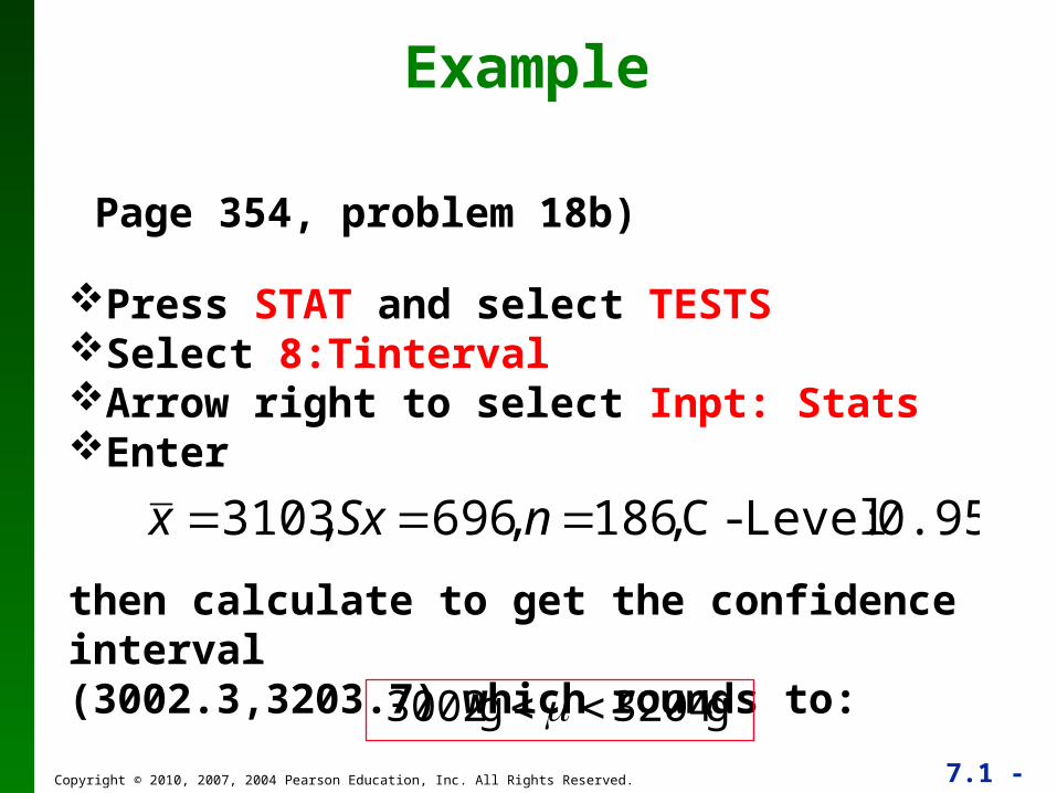
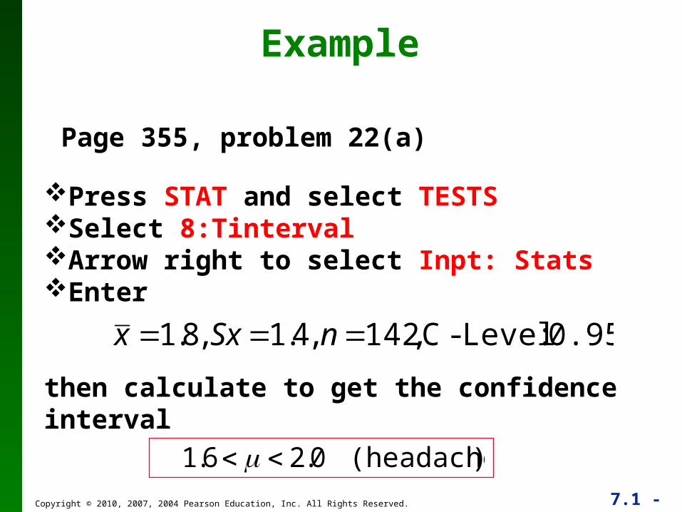
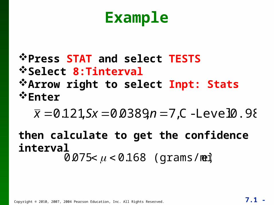
You will not be given Table A-3 on the exam and should be able to use your calculator to compute the confidence interval for population mean with σ unknown. This is the method that will be used for the remaining slides.

CALCULATOR


Example

Page 354

Problem 14:

NOTE: do part (b) first using the TI calculator


Example

The TI calculator will compute confidence intervals for population mean with σ unknown as follows:

Press STAT and select TESTSSelect 8:TintervalArrow right to select Inpt: StatsEnter ,Sx, n, C-Level and then calculate x


Example


ANSWER to part (b)

Press STAT and select TESTSSelect 8:TintervalArrow right to select Inpt: StatsEnter

Calculate then gives: (0.06395,0.17605)

0.99Level-C ,7 ,04.0 ,12.0 nSxx


Example


ANSWER to part (b)

We must round two decimal places (same number of places as the sample mean)

Units are grams/mile

18.006.0


Point estimate of µ:

x = (upper confidence limit) + (lower confidence limit)

2

Margin of Error:

E = upper confidence limit - x

Finding the Point Estimate and E from a Confidence Interval


Example


ANSWER to part (a) uses part (b)

18.006.0

grams/mile 12.02

18.006.0

x

grams/mile 06.012.018.0 E


Example



Example


a) ANSWER: grams 3103x


Example

Page 354, problem 18b)


then calculate to get the confidence interval(3002.3,3203.7) which rounds to:

0.95 :Level-C,186 ,696 ,3103 nSxx

g 3204 g 3002


Example


c) ANSWER:Yes, since the confidence interval

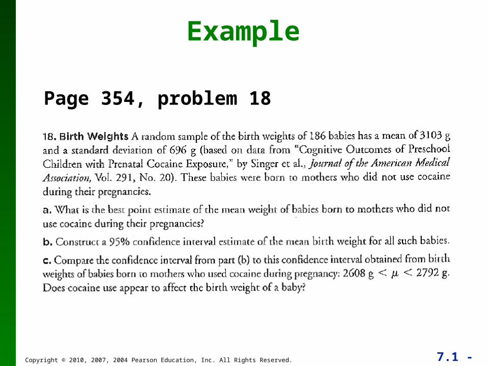
for the mean birth weight for mothers who used cocaine is entirely below the confidence interval in part (b) for mothers who did not use cocaine, it appears that cocaine use is associated with lower birth weights.

g 2792g 2608


Confidence Intervals for Comparing Data

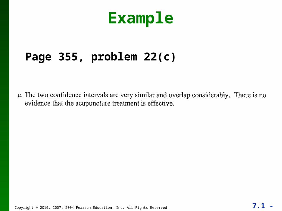
As in Sections 7-2 and 7-3, confidence intervals can be used informally to compare different data sets, but the overlapping of confidence intervals should not be used for making formal and final conclusions about equality of means.


Example



Example

Page 355, problem 22(a)


then calculate to get the confidence interval

0.95 :Level-C,142 ,4.1 ,8.1 nSxx

)(headaches 0.26.1


Example

Page 355, problem 22(b)



0.95 :Level-C,80 ,2.1 ,6.1 nSxx

)(headaches 9.13.1


Example

Page 355, problem 22(c)


Example



Example


Here:

and we are not given the mean and standard deviation. We must determine these from the given data.

0.98 :Level-C,7 ?, ,? nSxx


Example

Compute the mean:

g/mile 121.0 7

0.85

7

15.008.014.015.016.011.006.0

x

x =n

x


Example

Compute the standard deviation:

1

)( 2

n

xxs


Example

0.06 -0.061 0.003721

0.11 -0.011 0.000121

0.16 0.039 0.001521

0.15 0.029 0.000841

0.14 0.019 0.000361

0.08 -0.041 0.001681

0.15 0.029 0.000841

x xx 2)( xx

009087.0)( 2 xx

g/mile 0389.00015145.017

009087.0

s

Sum of last column:

3.1 - 122

•Calculator:

1)Enter the list of data values into a list using STAT 1:Edit

2)Select 2nd STAT (LIST) and arrow right to choose MATH option 3:mean(

3)Select 2nd STAT (LIST) and arrow right to choose MATH option 7:stdDev(

4)Choose the list the data is in


Example



0.98 :Level-C,7 ,0389.0 ,121.0 nSxx

e)(grams/mil 168.0075.0


Example



Recap

In this section we have discussed: Student t distribution. Degrees of freedom. Margin of error. Confidence intervals for μ with σ unknown. Choosing the appropriate distribution. Point estimates. Using confidence intervals to compare data.

Date post:	29-Dec-2015
Category:	Documents
Upload:	george-gordon
View:	215 times
Download:	2 times

7.1 - 1 Copyright © 2010, 2007, 2004 Pearson Education, Inc. All Rights Reserved. Chapter 7...

Documents