8-1 8. Adaptive Filters –Application in Equalization • References : 1. Sections 10.1, 10.2, 11.1.2,11.1.3, and 11.4.1 of the book Digital Communications , by J.G. Proakis, McGraw Hill, 4 th Edition, 2000. 2. S.S. Haykins, Adapative Filter Theory , 3 rd Edition, Prentice Hall, 1996. • A filter is a device that shapes the spectrum of the input signal in a certain manner. The general purpose of filtering is to enhance certain features of the input signal while suppressing the undesirable component or noise. • If the input signal is deterministic, then it is straight forward to design the filter, as we had seen in Chapters 5 and 6. Even if the input signal is random, we can still easily design an optimal filter, as long as the statistical information about the signal are available. This leads us to the so-called Weiner filter. However, if we have no prior information about the signal, then we can not optimally design the filter a priori. • The objective of this chapter is to discuss adaptive algorithms that can adjust the filter coefficients optimally when used to process an unknown signal.
Transcript
8-1
8. Adaptive Filters –Application in Equalization
• References:
1. Sections 10.1, 10.2, 11.1.2,11.1.3, and 11.4.1 of the book DigitalCommunications, by J.G. Proakis, McGraw Hill, 4th Edition, 2000.
• A filter is a device that shapes the spectrum of the input signal in a certainmanner.
The general purpose of filtering is to enhance certain features of the inputsignal while suppressing the undesirable component or noise.
• If the input signal is deterministic, then it is straight forward to design thefilter, as we had seen in Chapters 5 and 6.
Even if the input signal is random, we can still easily design an optimalfilter, as long as the statistical information about the signal are available.This leads us to the so-called Weiner filter.
However, if we have no prior information about the signal, then we can notoptimally design the filter a priori.
• The objective of this chapter is to discuss adaptive algorithms that canadjust the filter coefficients optimally when used to process an unknownsignal.
8-2
• While there are many applications for these adaptive filters, we focus onadaptive equalization of a digital communication signal in the pressence ofintersymbol interference (ISI).
8.1 The MMSE Equalizer
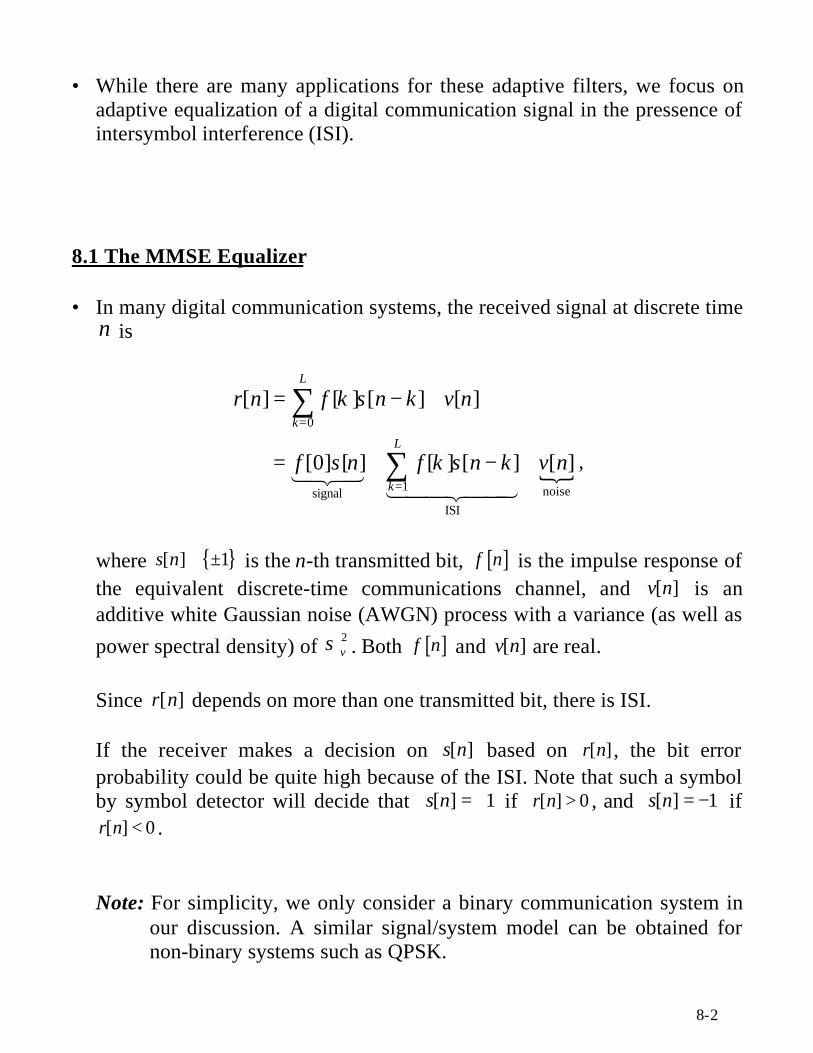
• In many digital communication systems, the received signal at discrete timen is
{
0
1 noisesignalISI
[ ] [ ] [ ] [ ]
[0] [ ] [ ] [ ] [ ]
L
k
L
k
r n f k s n k v n
f s n f k s n k v n
=
=
= − +
= + − +
∑
∑14243 1442443,
where { }[ ] 1s n ∈ ± is the n-th transmitted bit, [ ]f n is the impulse response ofthe equivalent discrete-time communications channel, and [ ]v n is anadditive white Gaussian noise (AWGN) process with a variance (as well as
power spectral density) of 2vσ . Both [ ]f n and [ ]v n are real.
Since [ ]r n depends on more than one transmitted bit, there is ISI.
If the receiver makes a decision on [ ]s n based on [ ]r n , the bit errorprobability could be quite high because of the ISI. Note that such a symbolby symbol detector will decide that [ ] 1s n = + if [ ] 0r n > , and [ ] 1s n = − if
[ ] 0r n < .
Note: For simplicity, we only consider a binary communication system inour discussion. A similar signal/system model can be obtained fornon-binary systems such as QPSK.
8-3
• To suppress ISI, we first pass the signal [ ]r n through an equalizer beforemaking decisions on the transmitted bits.
• There are many different types of equalizers. If we want to completelyeliminate the ISI in [ ]r n , we can use a zero-forcing equalizer.
Let ( ), ( ), ( ), and ( )R z S z F z V z be the respective z-transforms of [ ]r n , [ ]s n ,[ ]f n , and [ ]v n . Then
( ) ( ) ( ) ( )R z F z S z V z= + .
If we use a digital filter with a transfer function of
( ) 1/ ( )C z F z=
to filter [ ]r n , the output signal, [̂ ]s n , of the filter has a z-transform of
ˆ( ) ( ) ( )
( ) ( ) ( ) ( ) ( )
( ) ( ) ,
( )
S z C z R z
C z F z S z C z V z
V zS z
F z
== +
= +
which is free from ISI. Consequently, the filter ( )C z defined above iscalled a zero-forcing equalizer.
While the zero-forcing equalizer can completely eliminate ISI, it can leadto noise enhancement when ( ) 0jF e ω = at some ω . Because of this, thezero-forcing equalizer is not commonly used.
A more commonly used equalizer is the minimum mean square error(MMSE) equalizer.
8-4
• The MMSE equalizer is essentially a FIR filter with coefficients
1, ,...,K K Kc c c− − +
The input to the filter is the received signal [ ]r n and the output is the signal
[̂ ] [ ]K
kk K
s n c r n k=−
= −∑ .
The filter coefficients are chosen to minimize the mean square value of theequalization error
ˆ[ ] [ ] [ ]n s n s nε = − .
Note that after equalization, there will still be residual ISI. On top of that,there is an additive Gaussian noise term.
The MMSE equalizer minimizes the the combined residual ISI plus noisepower, which is different from the zero forcing equalizer that minimizesonly the ISI.
The non-casuality in the mathematical description of the MMSE equalizertranslates into a decision delay in the actual implementation.
• To obtain the filter coefficients of the MMSE equalizer, we first express allsignals involved in matrix form. Specifically, let
[ ][ 1]
[ ]
[ ]
r n K
r n Kn
r n K
+ + − = −
R M
8-5
be the received vector at time n and
( )1, ,...,K K Kc c c− − +=C
be a general transversal (i.e. FIR) equalizer. The equalizer output at timen is thus
[̂ ] [ ]s n n= CR
and the square equalization error is
( )( ) ( )
22
2
ˆ[ ] [ ] [ ]
[ ] [ ] [ ] [ ]
[ ] [ ] [ ] [ ] [ ] [ ] [ ]
1 [ ] [ ] [ ] [ ] [ ] [ ] ,
t t
t t t t
t t t t
n s n s n
s n n s n n
s n n s n s n n n n
n s n s n n n n
ε = −
= − −
= − − +
= − − +
CR R C
CR R C CR R C
CR R C CR R C
The mean square error (MSE) of the equalizer is
[ ][ ]
2[ ] 1 [ ] [ ] [ ] [ ] [ ] [ ]
1 [ ] [ ] [ ] [ ] [ ] [ ]
1
1 2
t t t t
t t t t
t tRs sR RR
tsR
E n E n s n E s n n E n n
E n s n E s n n E n n
γ ε = = − − + = − − +
= − − +
= −
CR R C CR R C
C R R C C R R C
Cu u C CU C
u C ,tRR+ CU C
where[ ] [ ]t t
sR RsE s n n = = u R u
is the correlation between [ ]s n and the received vector R[n], and
[ ] [ ]tRR E n n = U R R
is the covariance matrix of the received vector R[n].
8-6
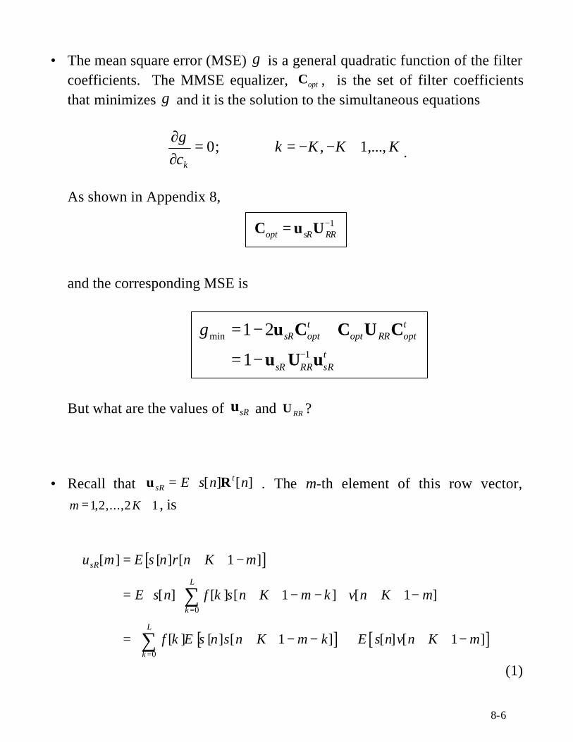
• The mean square error (MSE) γ is a general quadratic function of the filtercoefficients. The MMSE equalizer, optC , is the set of filter coefficientsthat minimizes γ and it is the solution to the simultaneous equations
0; , 1,...,k
k K K Kc
γ∂ = = − − +∂ .
As shown in Appendix 8,
and the corresponding MSE is
;
But what are the values of sRu and RRU ?
• Recall that [ ] [ ]tsR E s n n = u R . The m-th element of this row vector,
1,2,...,2 1m K= + , is
[ ]
[ ] [ ]
0
0
[ ] [ ] [ 1 ]
[ ] [ ] [ 1 ] [ 1 ]
[ ] [ ] [ 1 ] [ ] [ 1 ]
sR
L
k
L
k
u m E s n r n K m
E s n f k s n K m k v n K m
f k E s n s n K m k E s n v n K m
=
=
= + + −
= + + − − + + + −
= + + − − + + + −
∑
∑(1)
1opt sR RR
−=C u U
min
1
1 2
1
t tsR opt opt RR opt
tsR RR sR
γ−
= − +
= −
u C C U C
u U u
8-7
Assuming that different data bits are statistically independent, then
[ ] 1 [ ] [ ]
0
i jE s i s j
i j
== ≠
. (2)
Furthermore, the data bits are independent of the channel noise.Consequently,
[ ] [ ] [ ][ ] [ ] [ ] [ ] 0E s n v j E s n E v j= = . (3)
Substituting (2) & (3) into (1) yields
Example : When 4L = , 3K = (i.e. a 7-tap equalizer), we have
( )u [3], [2], [1], [0],0,0,0sR f f f f= .
However, when K is increased to 5, usR becomes
( )u 0, [4], [3], [2], [1], [0],0,0,0,0,0sR f f f f f= .
• The element on the thi − row and thj − column , 1,2,...,2 1i j K= + , of thecovariance matrix RRU is
[ ] [ ]
[ ]0
[ ] [ ] [ ] [ 1 ] [ ] [ 1 ]
1 if 0 1
0 otherwise
L
sRk
u m f k E s n s n K m k E s n v n K m
f K m K m L
=
= + + − − + + + −
+ − ≤ + − ≤
=
∑
8-8
[ ]
[ ]
0
0
0 0
[ , ] [ 1 ] [ 1 ]
[ ] [ 1 ] [ 1 ]
[ ] [ 1 ] [ 1 ]
[ ] [ ] [ 1 ] [ 1 ]
RR
L
k
L
m
L L
k m
u i j E r n K i r n K j
f k s n K i k v n K i
E
f m s n K j m v n K j
f k f m E s n K j m s n K i k
=
=
= =
= + + − + + −
+ + − − + + + − × = + + − − + + + −
= + + − − + + − −
∑
∑
∑∑
[ ]
[ ]0
0
[ ] [ 1 ] [ 1 ]
[ ] [ 1 ] [ 1 ]
[ 1 ] [ 1 ]
L
k
L
m
f k E s n K i k v n K j
f m E s n K j m v n K i
v n K i v n K j
=
=
+ + + − − + + −
+ + + − − + + −
+ + + − + + −
∑
∑
(4)
Substituting (2) & (3) into (4) yields
where it is understood that
[ ] 0[ ]
0 otherwise
f k i j k i j Lf k i j
+ − ≤ + − ≤+ − =
.
Note that [ ]nδ is the discrete-time impulse function and that the first term
in [ , ]RRu i j is actually the autorcorrelation function of the channel’simpulse response. We will denote it by
• In order to implement the MMSE equalizer in Section 8.1, the receiverneeds to know what the correlation vector sRu and the covariance matrix
RRU are. As shown earlier, these parameters depends on the channelconditions, namely the impulse response [ ]f n of the channel and the noisevariance 2
vσ .
• The channel conditions are usually unknown to the receiver prior to thecommunication session. Moreover, they may vary slowly with time after aconnection has been established.
What this means is that the receiver must estimate sRu and RRU online,either explicitly or implicitly.
• We present in this section an iterative procedure called the least meansquare (LMS) algorithm for determining the coefficients of a MMSEequalizer in an unknown channel.
The LMS algorithm is based on the method of steepest descent.
The key difference between the method of steepest descent and LMS is thatthe former uses the true gradient vector (which depends on the channelcondition) of the error surface γ in the iterations while the latter uses anestimate of the gradient vector.
The use of noisy gradients in the LMS algorithm leads to a MSE γ that isslightly larger than that of the true MMSE equalizer.
8-11
8.2.1 The Method of Steepest Descent
• As shown in Section 8.1, the general expression for the MSE γ of a
transversal equalizer ( )1, ,...,K K Kc c c− − +=C is
1 2 .t tsR RRγ = − +u C CU C
Since this term is a quadratic function of the kc s, there exists a globalminimum. As shown in Section 8.1, the location of the global minimum,i.e. the MMSE equalizer, is
1opt sR RR
−= =C C u U ,
• While the coefficients of the MMSE equalizer can be obtained throughdirect matrix inversion, they can also be obtained through an iterativemethod called the method of steepest descent.
Let [ ]nC be the estimate of optC at discrete-time (or iteration index) n. Thenbased on [ ]nC , we can obtain
( )[ ] 2 [ ]sR RRn n= − −G u C U ,
the gradient vector of the error surface γ at [ ]nC ; see the Appendix. Basedon [ ]nC and [ ]nG , we obtain the next estimate of optC according to
( )( )
[ 1] [ ] [ ]2
[ ] [ ]
[ ] ,sR RR
RR sR
n n n
n n
n
∆+ = −
= + ∆ −
= − ∆ + ∆
C C G
C u C U
C I U u
8-12
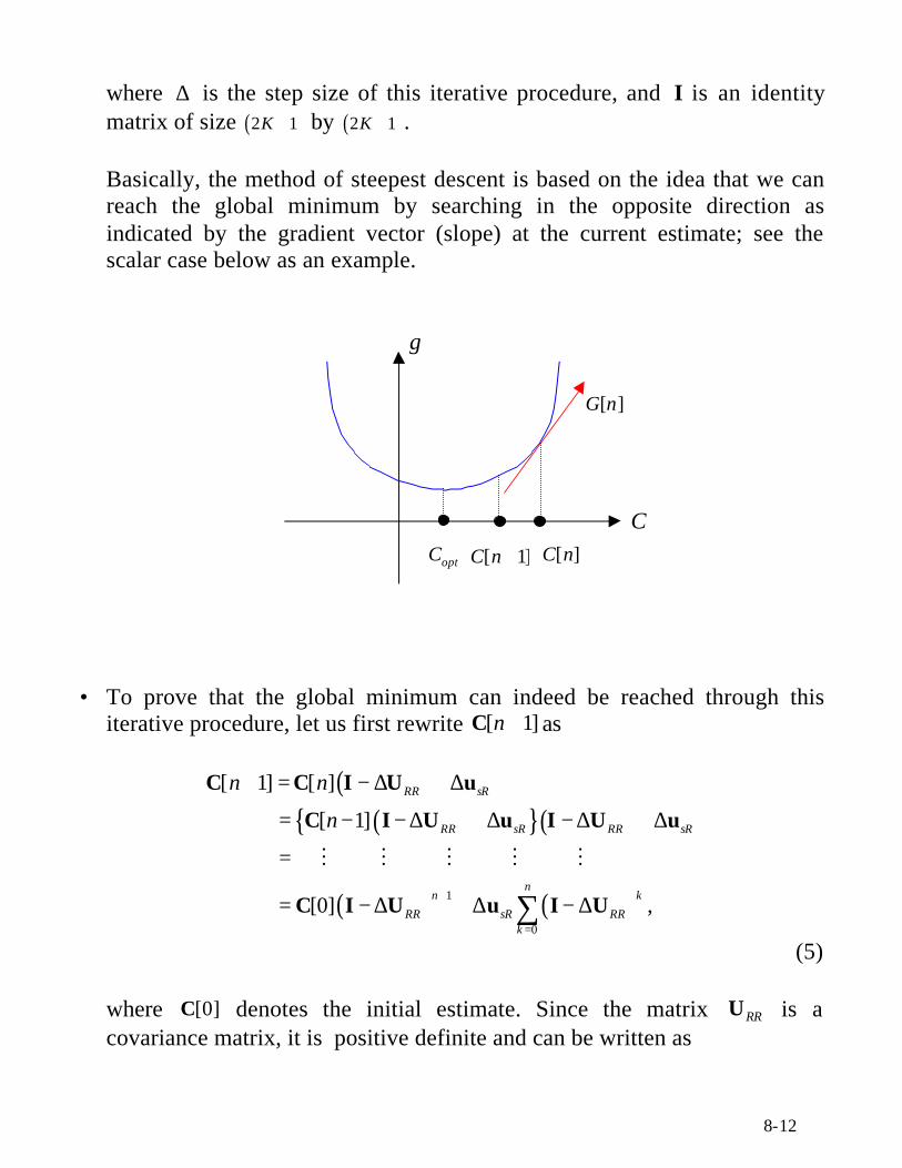
where ∆ is the step size of this iterative procedure, and I is an identitymatrix of size ( )2 1K + by ( )2 1K + .
Basically, the method of steepest descent is based on the idea that we canreach the global minimum by searching in the opposite direction asindicated by the gradient vector (slope) at the current estimate; see thescalar case below as an example.
• To prove that the global minimum can indeed be reached through thisiterative procedure, let us first rewrite [ 1]n +C as
( )( ){ }( )
( ) ( )1
0
[ 1] [ ]
[ 1]
[0] ,
RR sR
RR sR RR sR
nn k
RR sR RRk
n n
n
+
=
+ = − ∆ + ∆
= − − ∆ + ∆ − ∆ + ∆
=
= − ∆ + ∆ − ∆∑
C C I U u
C I U u I U u
C I U u I U
M M M M M
(5)
where [0]C denotes the initial estimate. Since the matrix RRU is acovariance matrix, it is positive definite and can be written as
[ 1]C n +
γ
[ ]G n
C
[ ]C noptC
8-13
tRR =U VDV ,
where V is a unitary matrix with the property
t t= =VV V V I ,
and
1
2
2 1K
λλ
λ +
=
D O
is a diagonal matrix containing all the eigenvalues of RRU . Note that
0; 0,1,...,2 1i i Kλ > = +
because RRU is positive definite, and that
1 1 tRR− −=U VD V
Based on these properties of RRU , we can express the terms RR− ∆I U and
( )k
RR− ∆I U in (5) as
( )
t tRR
t
t
− ∆ = − ∆
= − ∆
=
I U VV VDV
V I D V
VQV
and
( )k k tRR− ∆ =I U VQ V ,
8-14
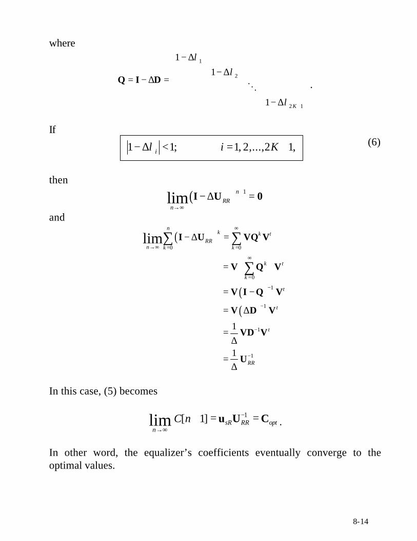
where
1
2
2 1
1
1
1 K
λλ
λ +
− ∆ − ∆ = − ∆ = − ∆
Q I D O .
If(6)
then
( ) 1lim n
RRn
+
→∞− ∆ =I U 0
and
( )
( )( )
0 0
0
1
1
1
1
limn
k k tRR
n k k
k t
k
t
t
t
∞
→∞ = =
∞
=
−
−
−
− ∆ =
=
= −
= ∆
=∆
∑ ∑
∑
I U VQ V
V Q V
V I Q V
V D V
VD V
11 RR
−=∆
U
In this case, (5) becomes
1 [ 1]lim sR RR optn
C n −
→∞+ = =u U C .
In other word, the equalizer’s coefficients eventually converge to theoptimal values.
1 1; 1, 2,...,2 1,i i Kλ− ∆ < = +
8-15
• Eqn (6) provides the requirements for the convergence of the steepestdescent algorithm. These requirements can be written alternatively as
20 ; 1,2,...,2 1
i
i Kλ
< ∆ < = + .
or simply
where maxλ is the largest eigenvalue of the covariance matrix RRU .
• For the steepest descent algorithm at hand, it is desirable to use a step sizeas close to the upper limit, max2 / λ , as possible. This guarantees the fastestconvergence rate possible. However, for the LMS algorithm discussed inSection 8.2.2, using too large a step size will increase the MSE of theequalizer.
• Assume we select a step size of
max2/ λ +∆ = ,
where maxλ + is a number slightly greater than maxλ . Then the absolute valuesof the elements of the diagonal matrix 1 1( )n n+ += − ∆Q I D are
11
max
21 1 ; 1,2,...,2 1
nn i
i i Kλ
λλ
++
+− ∆ = − = + .
max
20 ,
λ< ∆ <
8-16
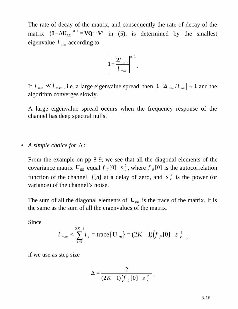
The rate of decay of the matrix, and consequently the rate of decay of thematrix ( ) 1 1n n t
RR
+ +− ∆ =I U VQ V in (5), is determined by the smallesteigenvalue minλ according to
1
min
max
21
nλ
λ
+
+− .
If min maxλ λ= , i.e. a large eigenvalue spread, then min max1 2 / 1λ λ− → and thealgorithm converges slowly.
A large eigenvalue spread occurs when the frequency response of thechannel has deep spectral nulls.
• A simple choice for ∆ :
From the example on pp 8-9, we see that all the diagonal elements of thecovariance matrix RRU equal 2[0]ff vφ σ+ , where [0]ffφ is the autocorrelation
function of the channel [ ]f n at a delay of zero, and 2vσ is the power (or
variance) of the channel’s noise.
The sum of all the diagonal elements of RRU is the trace of the matrix. It isthe same as the sum of all the eigenvalues of the matrix.
Since
{ } ( )2 1
2max
1
trace (2 1) [0]K
i RR ff vi
Kλ λ φ σ+
=
< = = + +∑ U ,
if we use as step size
( )2
2(2 1) [0]ff vK φ σ
∆ =+ + .
8-17
then it is guaranteed that max2 / λ∆ < .
For the LMS algorithm discussed in the next section, it is import to make∆ substantially smaller than ( ){ }22 / (2 1) [0]ff vK φ σ+ + so that the excess MSE isrelatively small compared to the MSE of the MMSE equalizer.
8.2.2 The LMS Algorithm
• While the steepest descent method is able to determine the optimalequalizer coefficients without performing any matrix inversion, itsoperation is still based on the assumption that the channel parameters sRu
and RRU are known to the receiver. Recall that the receiver uses theseparameters to compute the gradient vector [ ]nG required for updating thethe equalizer coefficients.
• In the LMS algorithm, the gradient vector is replaced by its estimate.
• Let us consider the correlation of the received vector [ ]nR on pp 8-4 withthe equalization error
ˆ[ ] [ ] [ ] [ ] [ ]n s n s n s n nε = − = −CR
for the equalizer C. The result is
8-18
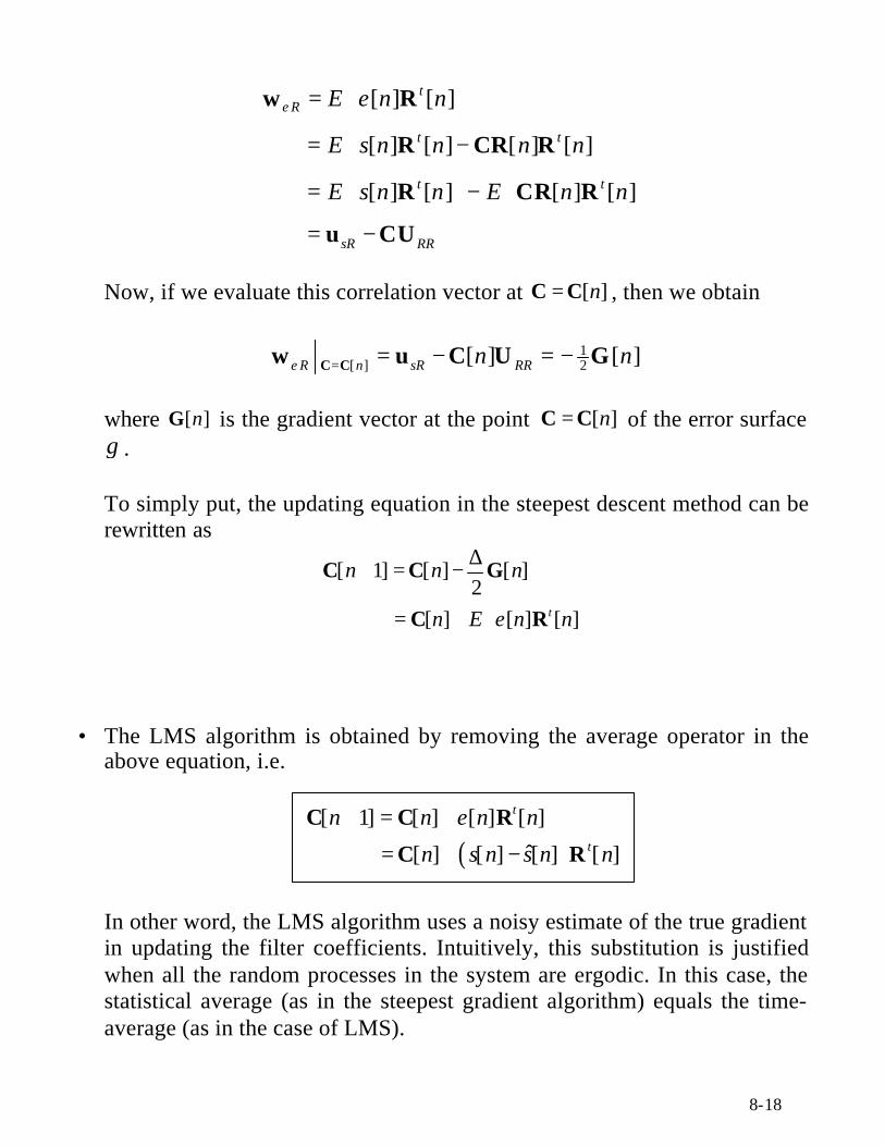
[ ] [ ]
[ ] [ ] [ ] [ ]
[ ] [ ] [ ] [ ]
tR
t t
t t
sR RR
E n n
E s n n n n
E s n n E n n
ε ε = = − = −
= −
w R
R CR R
R CR R
u CU
Now, if we evaluate this correlation vector at [ ]n=C C , then we obtain
1[ ] 2[ ] [ ]R n sR RRn nε = = − = −C Cw u C U G
where [ ]nG is the gradient vector at the point [ ]n=C C of the error surfaceγ .
To simply put, the updating equation in the steepest descent method can berewritten as
[ 1] [ ] [ ]2
[ ] [ ] [ ]t
n n n
n E n nε
∆+ = −
= +
C C G
C R
• The LMS algorithm is obtained by removing the average operator in theabove equation, i.e.
In other word, the LMS algorithm uses a noisy estimate of the true gradientin updating the filter coefficients. Intuitively, this substitution is justifiedwhen all the random processes in the system are ergodic. In this case, thestatistical average (as in the steepest gradient algorithm) equals the time-average (as in the case of LMS).
( )[ 1] [ ] [ ] [ ]
ˆ [ ] [ ] [ ] [ ]
t
t
n n n n
n s n s n n
ε+ = +
= + −
C C R
C R
8-19
• Notice that the LMS-based equalizer does not need any information aboutthe channel to update its coefficients.
The algorithm however does require knowledge of the transmitted symbols,which are supposed to be unknown to the receiver. In practice, we can getaround this problem by using the detected symbol [ ]s n% instead of [ ]s nwhen we update the equalizer coefficients. Note that
ˆ1 if [ ] 0[ ]
ˆ1 if [ ] 0
s ns n
s n
+ >= − <
% .
Furthermore, we can send an initial training sequence to help the equalizerconverges quickly. The symbols in the training sequence will be known tothe receiver. However, frame/bit sync are required in order for the receiverto locate the training pattern.
• The use of noisy gradients in the adaptation process results in excess MSE.Specifically, the MSE of a LMS-based adaptive transversal equalizer is
minγ γ γ ∆≈ + ,
where minγ is the MMSE defined on pp 8-6, and
( )21min2 (2 1) [0]ff vKγ φ σ γ∆ ≈ ∆ + +
is the excess MSE.
In order to make γ∆ substantially smaller than minγ while maintaing areasonable convergence rate, the step size ∆ should only be a fraction of
( ){ }22 / (2 1) [0]ff vK φ σ+ + . For example, when
8-20
( ) ( )2 2
1 2 0.210 (2 1) [0] (2 1) [0]ff v ff vK Kφ σ φ σ
∆ = =
+ + + + ,
then min0.1γ γ∆ = and the increase in total MSE is
min10
min
10log 0.414 dBγ γ
γ∆ + =
As shown in Section 8.2.1, using a step size of ( ){ }22 / (2 1) [0]ff vK φ σ+ + orsmaller will gurantee convergence.
• Example : A LMS-based equalizer with 2 1 11K + = taps is used to suppressISI in a communication channel with an eigenvalue spread of max min/ 11λ λ =
and a combined signal plus noise power of 2[0] 1ff vφ σ+ = . The largest stepsize that can be used while ensuring that the excess MSE does not exceedthe MMSE is
( )( )2
20.18
2 1 [0]ff vK φ σ∆ = =
+ +
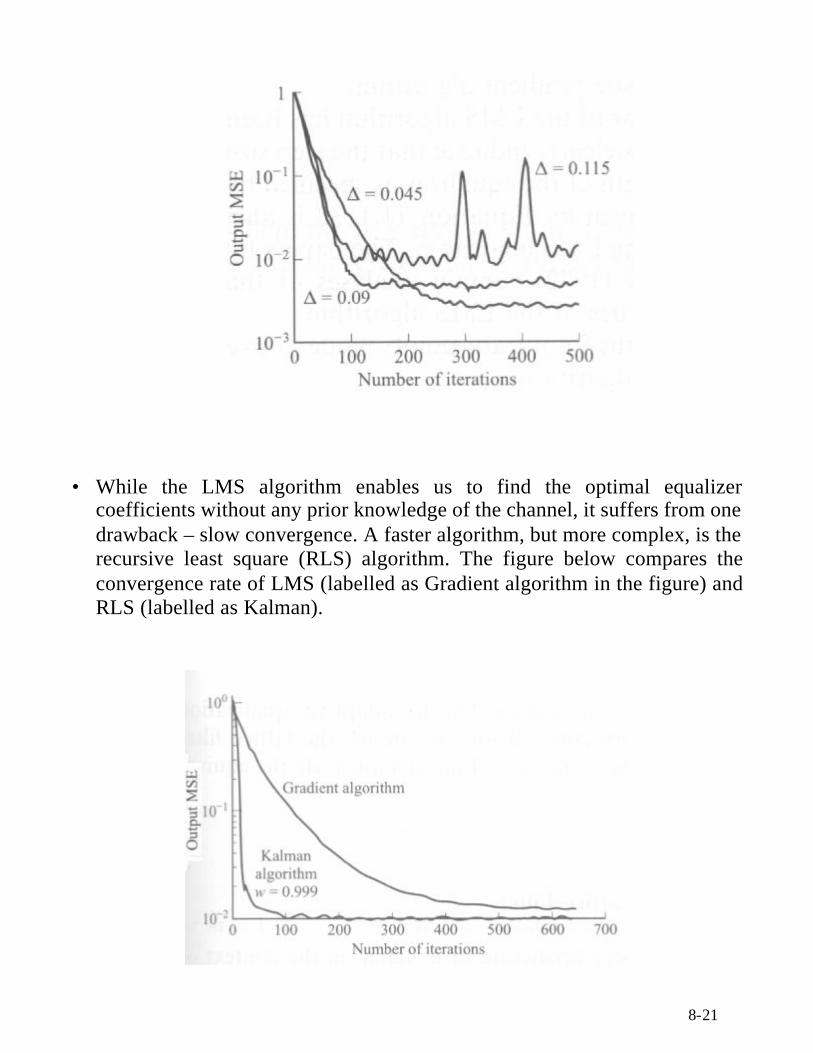
The figure below plots the MSE of the equalizer as a function of theiteration number with ∆ as a parameter (the results were obtained over 200simulation runs).
It is observed that in general, the larger the step size is, the faster the initialconvergence. However, the steady state MSE will be larger as well.
For the three step sizes considered, 0.09∆ = (or half the upperbound above)provides the best tradeoff between MSE and rate of convergence.
8-21
• While the LMS algorithm enables us to find the optimal equalizercoefficients without any prior knowledge of the channel, it suffers from onedrawback – slow convergence. A faster algorithm, but more complex, is therecursive least square (RLS) algorithm. The figure below compares theconvergence rate of LMS (labelled as Gradient algorithm in the figure) andRLS (labelled as Kalman).
8-22
Appendix 8
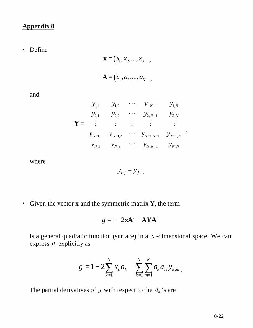
• Define( )1 2, ,..., Nx x x=x ,
( )1 2, ,..., Na a a=A ,
and
1,1 1,2 1, 1 1,
2,1 2,2 2, 1 2,
1,1 1,2 1, 1 1,
,1 ,2 , 1 ,
N N
N N
N N N N N N
N N N N N N
y y y y
y y y y
y y y y
y y y y
−
−
− − − − −
−
=
Y
LL
M M M M MLL
,
where
, ,i j j iy y= .
• Given the vector x and the symmetric matrix Y, the term
1 2 t tγ = − +xA AYA
is a general quadratic function (surface) in a N -dimensional space. We canexpress γ explicitly as
,1 1 1
1 2N N N
k k k m k mk k m
x a a a yγ= = =
= − +∑ ∑∑ .
The partial derivatives of γ with respect to the ka ’s are
8-23
,1
2 2 ; 1, 2,...,N
i k k iki
x a y i Na
γ=
∂ = − + =∂ ∑
These partial derivatives can be grouped together to form the gradientvector
1 2
, ,...,
2 2Na a a
γ γ γ ∂ ∂ ∂= ∂ ∂ ∂ = − +
G
x AY
The gradient vector is the tangent of the N-dimensional surface γ at thepoint A . When the gradient vector is zero, the surface γ reaches its lowestvalue. The point in the N-dimensional space where this occurs is
1opt
−= =A xY A .
In the context of the MMSE equalizer in Section 8.1, γ is the mean squareequalization error, sR≡x u , RR≡Y U , and ≡A C . The objective is to findthe set of filter coefficients that minimizes γ . Based on the general resultsderived in this Appendix, it can be easily deduce that the MMSE equalizeris
(A1)
Moreover, the gradient G of the error surface γ at the (non-optimal)equalizer setting of C is
(A2)
Eqn (A2) will be useful later on when we discuss the gradient and thestochastic gradient (LMS) algorithms for automatic adjustment of theequalization filter.