8 Anisotropic aquifers The standard methods of analysis are all based on the assumption that the aquifer is isotropic, i.e. that the hydraulic conductivity is the same in all directions. Many aquifers, however, are anisotropic. In such aquifers, it is not unusual to find hydraulic conductivities that differ by a factor of between two and twenty when measured in one or another direction. Anisotropy is a common feature in water-laid sedimentary deposits (e.g. fluvial, clastic lake, deltaic and glacial outwash deposits). Aquifers that are composed of water-laid deposits may exhibit anisotropy on the horizontal plane. The hydraulicconductivity in the direction of flow tends to be greater than that perpen- dicular to flow. Because of the differences in hydraulic conductivity, lines of equal drawdown around a pumped well in these aquifers will form ellipses rather than con- centric circles. In addition such aquifers are often stratified, i.e. they are made up of alternating layers ofcoarse and fine sands, gravels, and occasional clays, with each layer possessing a unique value of K. Any layer with a low K will retard vertical flow, but horizontal flow can occur easily through any layer with relatively high K. Obviously, K,, i.e. parallel to the bedding planes, will be much higher than K,, and the aquifer is said to be anisotropic on the vertical plane. Aquifers that are anisotropic on both the horizontal and vertical planes, are said to exhibit three-dimensional anisotropy, with principal axes of K in the vertical direc- tion, the horizontal direction parallel to stream flows that prevailed in the past, and the horizontal direction at a right angle to those flows. It will be clear that, in the analysis of pumping tests, anisotropy poses a special problem. Methods of analysis that take anisotropy on the horizontal plane into account are presented in Section 8.1 for confined aquifers and in Section 8.2 for leaky aquifers. Sections 8.3, 8.4 and 8.5 discuss anisotropy on the vertical plane in confined aquifers, leaky aquifers, and unconfined aquifers. 8.1 Confined aquifers, anisotropic on the horizontal plane 8.1.1 Hantush’s method The unsteady-state drawdown in a confined isotropic aquifer is given by the Theis equation (Equation 3.5) s=- W(U> 47tKD where r2S 4KDt u=- In a confined aquifer that is anisotropic on the horizontal plane, with the principal 133
Transcript
8 Anisotropic aquifers
The standard methods of analysis are all based on the assumption that the aquifer is isotropic, i.e. that the hydraulic conductivity is the same in all directions. Many aquifers, however, are anisotropic. In such aquifers, it is not unusual to find hydraulic conductivities that differ by a factor of between two and twenty when measured in one or another direction. Anisotropy is a common feature in water-laid sedimentary deposits (e.g. fluvial, clastic lake, deltaic and glacial outwash deposits). Aquifers that are composed of water-laid deposits may exhibit anisotropy on the horizontal plane. The hydraulicconductivity in the direction of flow tends to be greater than that perpen- dicular to flow. Because of the differences in hydraulic conductivity, lines of equal drawdown around a pumped well in these aquifers will form ellipses rather than con- centric circles.
In addition such aquifers are often stratified, i.e. they are made up of alternating layers ofcoarse and fine sands, gravels, and occasional clays, with each layer possessing a unique value of K. Any layer with a low K will retard vertical flow, but horizontal flow can occur easily through any layer with relatively high K. Obviously, K,, i.e. parallel to the bedding planes, will be much higher than K,, and the aquifer is said to be anisotropic on the vertical plane.
Aquifers that are anisotropic on both the horizontal and vertical planes, are said to exhibit three-dimensional anisotropy, with principal axes of K in the vertical direc- tion, the horizontal direction parallel to stream flows that prevailed in the past, and the horizontal direction at a right angle to those flows.
It will be clear that, in the analysis of pumping tests, anisotropy poses a special problem. Methods of analysis that take anisotropy on the horizontal plane into account are presented in Section 8.1 for confined aquifers and in Section 8.2 for leaky aquifers. Sections 8.3, 8.4 and 8.5 discuss anisotropy on the vertical plane in confined aquifers, leaky aquifers, and unconfined aquifers.
8.1 Confined aquifers, anisotropic on the horizontal plane
8.1.1 Hantush’s method
The unsteady-state drawdown in a confined isotropic aquifer is given by the Theis equation (Equation 3.5)
s = - W(U> 47tKD
where
r2S 4KDt
u = -
In a confined aquifer that is anisotropic on the horizontal plane, with the principal
133
axes of anisotropy X and Y, the above equations, according to Hantush (1966), are replaced by
where
(KD), = ,/(KD)x x (KD), = the effective transmissivity (8.3) (KD), = transmissivity in the major direction of anisotropy (KD)y = transmissivity in the minor direction of anisotropy (KD), = transmissivity in a direction that makes an angle (0 + a) with the
X axis (0 and a will be defined below)
If we have one or more piezometers on a ray that forms an angle (0 + a) with the X axis, we can apply the methods for isotropic aquifers and obtain values for (KD), and S/(KD),. Consequently, to calculate S and (KD),, we need data from more than one ray of piezometers.
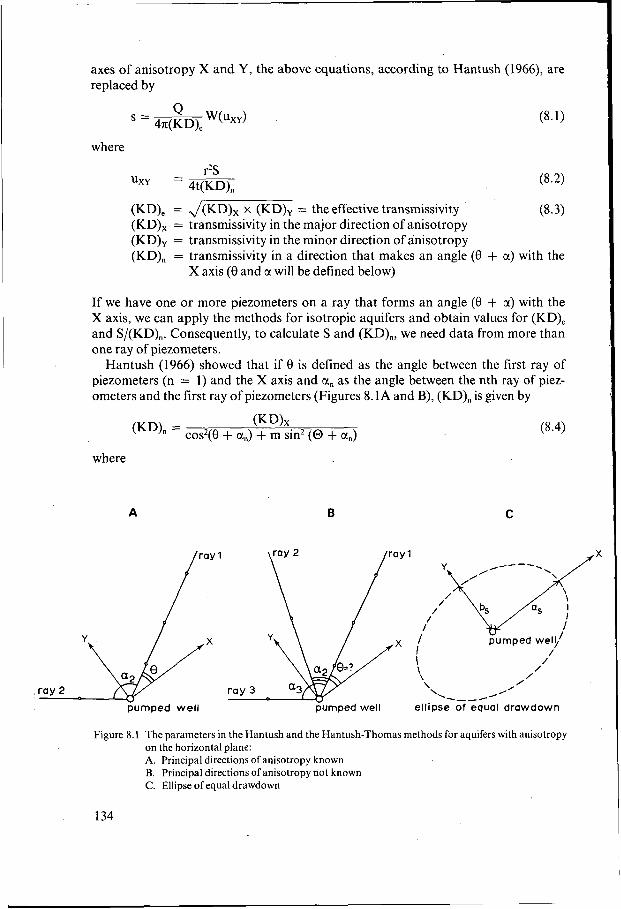
Hantush (1966) showed that if 0 is defined as the angle between the first ray of piezometers (n = 1) and the X axis and a, as the angle between the nth ray of piez- ometers and the first ray of piezometers (Figures 8.1 A and B), (KD), is given by
where
A B
1
pumped well
C
/ /
/ Í '1 / \ / '----- //'
ellipse of equal drawdown
Figure 8.1 The parameters in the Hantush and the Hantush-Thomas methods for aquifers with anisotropy on the horizontal plane: A. Principal directions of anisotropy known B. Principal directions of anisotropy not known C. Ellipse of equal drawdown
134
I (8.5) I I I
Because a, = O for the first ray of piezometers, Equation 8.4 reduces to
and consequently
(KD), - cos2(@ + a,) + m sin2@ + a,) - cos2 8 + m sin2 8 a, = -
(KD)n It goes without saying that a, = 1. A combination of Equations 8.5 and 8.7 yields
(8.7)
If the principal directions of anisotropy are not known, one needs at least three piez- ometers on different rays from the pumped well to solve Equation 8.7 for 8, using
Equation 8.9 has two roots for the angle (2 0) in the range O to 271 of the XY plane. If one of the roots is 6, the other will be 7c + 6. Consequently, 8 has two values: 6/2 and (71 + 6)/2. One of the values of 8 yields m > 1 and the other m < 1 . Since the X axis is assumed to be along the major axis of anisotropy, the value of 8 that will make m = (KD)x/(KD)y > 1 locates the major axis of anisotropy, X; the other value locates the minor axis of anisotropy, Y. (It should be noted that a negative value of8 indicates that the positive X axis lies to the left of the first ray of piezometers.) The Hantush method can be applied if the following assumptions and conditions are satisfied: - The assumptions listed at the beginning of Chapter 3, with the exception of the
third assumption, which is replaced by: The aquifer is homogeneous, anisotropic on the horizontal plane, and of uniform thickness over the area influenced by the pumping test.
The following conditions are added: - The flow to the well is in unsteady state; - If the principal directions of anisotropy are known, drawdown data from two piez-
ometers on different rays from the pumped well will be sufficient. If the principal directions of anisotropy are not known, drawdown data must be available from at least three rays of piezometers.
Procedure 8.1 (principal directions of anisotropy known) - Apply the methods for isotropic confined aquifers (Sections 3.2.1 and 3.2.2) to the
data ofeach ofthe two rays ofpiezometers. This results in values for(KD),, S/(KD),, and S/(KD),;
- A combination of the last two values gives a, (cf. Equation 8.7). Because 8 and a, are known, substitute the values of 8, a, a, and (KD), into Equation 8.8 and
135 calculate m;
- Knowing (KD), and m, calculate (KD), and (KD), from Equation 8.5; - Substitute the values of (KD),, m, 0, and a2 into Equations 8.6 and 8.7 and solve
- A combination of the last two values with those for S/(KD), and S/(KD),, respective- for (KD), and (KD)2 ;
ly, yields values for S, which should be essentially the same.
Procedure 8.2 (principal directions of anisotropy unknown) - Apply the methods for isotropic confined aquifers (Sections 3.2.1 and 3.2.2) to the
data from each of the three rays of piezometers. This results in values for (KD),,
- A combination of S/(KD), with S/(KD), and S/(KD),, respectively, yields values for a, and a3. Because a’ and ci3 are known, 0 can be calculated from Equation 8.9;
- Substitute the values of 0, (KD),, ci2, and a, (or a, and a3) into Equation 8.8 and calculate m;
- Knowing (KD), and m, calculate (KD), and (KD), from Equation 8.5; - Substitute the values of (KD),, m, and 0 and the values of a, = O, a‘, and a, into
- A combination of these values with those of S/(KD),, S/(KD),, and S/(KD),, respec-
S/(KD)l, S/(KD)’, and S/(KD),;
Equation 8.4 and solve for (KD),, (KD),, and (KD),;
tively, yields values for S, which should be essentially the same.
Remarks - The observed data should permit the use of those methods for isotropic confined
aquifers that give a value for S/(KD),. Hence, the methods for steady-state flow in isotropic confined aquifers (Section 3.1) are not applicable;
- The analysis of the data from each ray of piezometers yields a value of (KD),. These values should all be essentially the same.
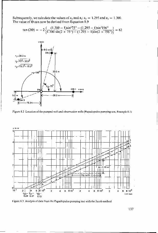
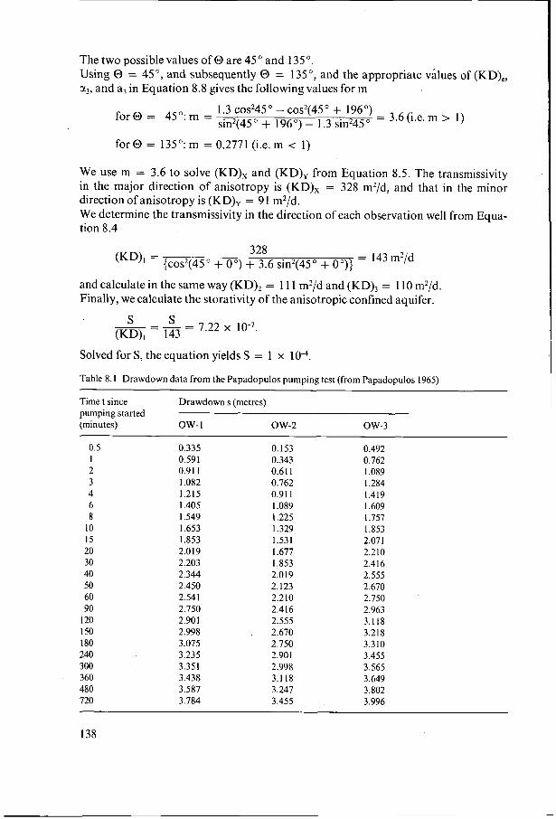
Example 8.1 Using Procedure 8.2, we shall analyse the drawdown data presented by Papadopulos (1965). The data are from a pumping test conducted in an anisotropic confined aquifer. During the test, the well PW was pumped at a discharge rate of 1086 m3/d. The draw- down was observed in three observation wells OW-l, OW-2, and OW-3, located as shown in Figure 8.2.
For each observation well, we plot the drawdown data on semi-log paper (Figure 8.3). The data allow the application of Jacob’s straight line method (Chapter 3) to determine the values of (KD), and S/(KD),, S/(KD),, and S/(KD),
(KD), = - - - 2.304 2.30 x 1086 47cAs = 173m2,d 4 x 3.14 x 1.15
2’25 - 9.35 x 10⁻⁷d/m2 S - 2.25 to’ - (KD), r2 (92 + 33.5’) x 1440 -
- 9.39 x IO-’d/m2 s - 2.25 to, - 2.25 x 0.24 (KD), r’ (19.3’ + 5.2’) x 1440 -
136
Subsequently, we calculate the values of a, and a3: a2 = 1.295 and a3 = 1.300. The value of 0 can now be derived from Equation 8.9
(1.300 - l)sin275" - (1.295 - l)sin2196" = 82 tan (20) = -2 (1.300 sin(2 x 75") - (1.295 - l)sin(2 x 196")]
V -
03=196'
f , 5.2 m .
I
OW-2. -9.0 ll+
I I :T 28.3 m-j
Figure 8.2 Location of the pumped well and observation wells (Papadopulos pumping test, Example 8.1)
137
The two possible values of O are 45 O and 135 O.
Using O = 45", and subsequently O = 135", and the appropriate values of (KD),, CY,, and a3 in Equation 8.8 gives the following values form
= 3.6(i.e.m > 1) 1.3 cos245 O - cos2(45 O + 196 ") sin2(45 O + 196") - 1.3 sin245 O
for@ = 45":m =
for O = 135": m = 0.2771 (i.e. m < 1)
We use m = 3.6 to solve (KD)x and (KD), from Equation 8.5. The transmissivity in the major direction of anisotropy is (KD), = 328 m2/d, and that in the minor direction of anisotropy is (KD), = 91 m2/d. We determine the transmissivity in the direction of each observation well from Equa- tion 8.4
In an isotropic aquifer, the lines of equal drawdown around a pumped well form con- centric circles, whereas in an aquifer that is anisotropic on the horizontal plane, those lines form ellipses, which satisfy the equation
(8.10)
where a, and b, are the lengths of the principal axes of the ellipse of equal drawdown s at the time t, (Figure 8. IC). It can be shown that
47cs(KD), Q = WUXY)
where
(8.1 1)
(8.12)
(8.13)
(8.14)
(8.15)
Hantush and Thomas (1966) stated that when (KD),, a,, and b, are known the other hydraulic characteristics can be calculated. Hence, it is not necessary to have values of S/(KD),, provided that one has sufficient observations to draw the ellipses of equal drawdown.
The Hantush-Thomas method can be applied if the following assumptions and condi- tions are satisfied: - The assumptions listed at the beginning of Chapter 3, with the exception of the
third assumption, which is replaced by: The aquifer is homogeneous, anisotropic on the horizontal plane, and of uniform thickness over the area influenced by the pumping test.
The following condition is added: - The flow to the well is in unsteady state.
Procedure 8.3 - Apply the methods for isotropic confined aquifers (Sections 3.1 and 3.2) to the data
from each ray of piezometers; this yields values for (KD), and sometimes S/(KD),. The factor (KD), is constant for the whole flow system, and S/(KD), is constant along each ray;
- Substitute the values of (KD), and S/(KD)" into Equations 8.1 and 8.2 and calculate the drawdown at any desired time and at any distance along each ray of piezometers;
- Construct one or more ellipses of equal drawdown (Figure 8.lC), using observed (or calculated) data, and calculate for each ellipse a, and b,;
- Calculate (KD),, (KD),, and (KD)Y from Equations 8.1 1 to 8.13;
139
- Calculate the value of W(u,,) from Equation 8.14 and find the corresponding value of uxy from Annex 3.1 ; With the value of uxy known, calculate S from Equation 8.15;
the same values for (KD),, (KD),, (KD),, and S. - Repeat this procedure for several values of s. This should produce approximately
8.1.3 Neuman’s extension of the Papadopulos method
In aquifers that are anisotropic on the horizontal plane, the orientation of the hydrau- lic-head gradients and the flow velocity seldom coincide; the flow tends to follow the direction of the highest permeability. This leads us to regard the hydraulic conductivity as a tensorial property, which is simply the mathematical translation of our observa- tion of the non-coincidence. Regarding the hydraulic conductivity in this way, we must define the tensor K, which is a matrix of nine coefficients, symmetrical to the diagonal. This allows us to transform the components of the hydraulic gradient into components of velocity. Along the principal axes of such a tensor (X,Y), the velocity and hydraulic gradients have the same directions.
By making use of the tensor properties, Papadopulos (1965) developed an equation for the unsteady-state drawdown induced in a confined aquifer that is anisotropic on the horizontal plane
(8.16)
where
(KD),,y2 + (KD),,x2 - 2(KD),,xy 4t (KD),2
(8.17)
where x and y are local coordinates (Figure 8.4) and (KD),,, (KD),,, and (KD),, are components of the transmissivity tensor.
where X and Y are global coordinates of the transmissivity tensor (Figure 8.4). The X axis is parallel to the major direction of anisotropy; the Y axis is parallel
140
0 pumped well piezometer
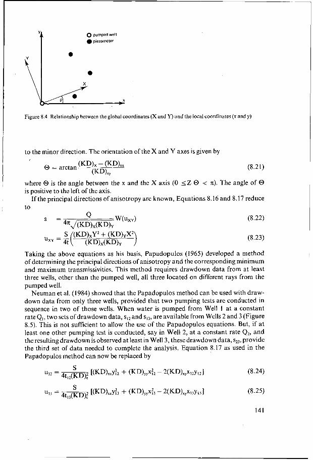
Figure 8.4 Relationship between the global coordinates (X and Y) and the local coordinates (x and y)
to the minor direction. The orientation of the X and Y axes is given by
(8.21)
where O is the angle between the x and the X axis (O I Z O < n). The angle of O is positive to the left of the axis.
If the principal directions of anisotropy are known, Equations 8.16 and 8.17 reduce to
(8.22)
(8.23)
Taking the above equations as his basis, Papadopulos ( I 965) developed a method of determining the principal directions of anisotropy and the corresponding minimum and maximum transmissivities. This method requires drawdown data from at least three wells, other than the pumped well, all three located on different rays from the pumped well.
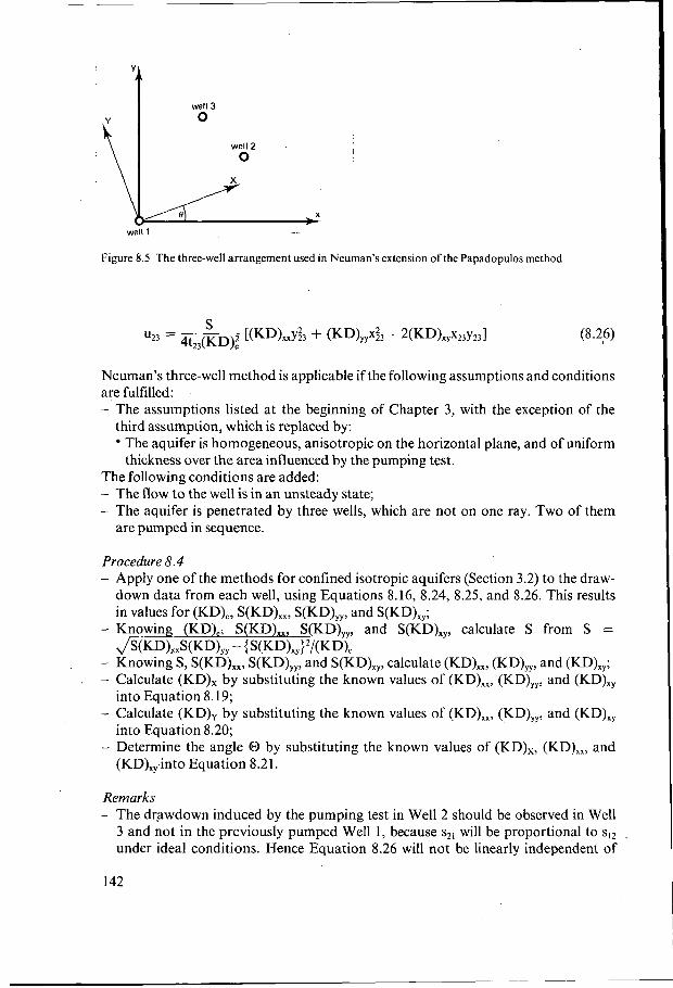
Neuman et al. (1984) showed that the Papadopulos method can be used with draw- down data from only three wells, provided that two pumping tests are conducted in sequence in two of those wells. When water is pumped from Well 1 at a constant rate Q,, two sets of drawdown data, s , ~ and s13, are available from Wells 2 and 3 (Figure 8.5). This is not sufficient to allow the use of the Papadopulos equations. But, if at least one other pumping test is conducted, say in Well 2, at a constant rate Q2, and the resulting drawdown is observed a t least in Well 3, these drawdown data, ~ 2 3 , provide the third set of data needed to complete the analysis. Equation 8.17 as used in the Papadopulos method can now be replaced by
(8.25)
141
V I
well 3
well 2
X
X L -
I
_- well 1 . .
Figure 8.5 The three-well arrangement used in Neuman’s extension of the Papadopulos method
Neuman’s three-well method is applicable if the following assumptions and conditions are fulfilled: - The assumptions listed at the beginning of Chapter 3, with the exception of the
third assumption, which is replaced by: The aquifer is homogeneous, anisotropic on the horizontal plane, and of uniform thickness over the area influenced by the pumping test.
The following conditions are added: - The flow to the well is in an unsteady state; - The aquifer is penetrated by three wells, which are not on one ray. Two of them
are pumped in sequence.
Procedure 8.4 - Apply one of the methods for confined isotropic aquifers (Section 3.2) to the draw-
down data from each well, using Equations 8.16, 8.24, 8.25, and 8.26. This results in values for (KD),, S(KD),,, S(KD),, and S(KD),,;
- Knowing (KD),, S(KD),, S(KD),,, and S(KD),,, calculate S from S =
- inowing S, S(KD),,, S(KD),,, and S(KD),,, calculate (KD),,, (KD),,, and (KD),,; - Calculate (KD), by substituting the known values of (KD),,, (KD),,, and (KD),,
- Calculate (KD), by substituting the known values of (KD),,, (KD),,, and (KD),,
- Determine the angle O by substituting the known values of (KD),, (KD),,, and
S(KD),xS(KD),,- {S(KD)x,)2/(KD)e
into Equation 8.19;
into Equation 8.20;
(KD),,,into Equation 8.21.
Remarks - The drawdown induced by the pumping test in Well 2 should be observed in Well
3 and not in the previously pumped Well 1, because s21 will be proportional to sI2 under ideal conditions. Hence Equation 8.26 will not be linearly independent of
142
Equation 8.24 and no unique solutions can be found for the Equations 8.24, 8.25, and 8.26;
- According to Neuman et al. (1984), more reliable results can be obtained by conduct- ing three pumping tests, pumping one well at a time and observing the drawdown in the other two wells. Equation 8.17 should then be replaced in the calculations by up to six equations of the form
where i, j = 1,2, 3. A least-squares procedure can be used to solve these equations and determine
‘ S(KD),,, S(KD),,, and S(KD),,. (For more information, see Neuman et al. 1984); - If drawdown data are available from at least three piezometers or observation wells
on different rays from the pumped well, the Papadopulos method can be used. The procedure is the same as Procedure 8.4, except that in the first step of Procedure 8.4, Equation 8.18 should be used instead of Equations 8.24,8.25, and 8.26 to deter- mine the values of S(KD),,, S(KD),,, and S(KD),,.
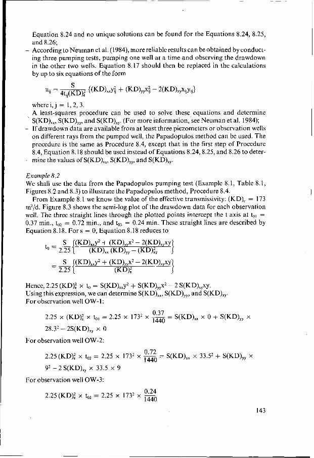
Example 8.2 We shall use the data from the Papadopulos pumping test (Example 8.1, Table 8.1, Figures 8.2 and 8.3) to illustrate the Papadopulos method, Procedure 8.4.
From Example 8.1 we know the value of the effective transmissivity: (KD), = 173 m2/d. Figure 8.3 shows the semi-log plot of the drawdown data for each observation well. The three straight lines through the plotted points intercept the t axis at to, = 0.37 min., to’ = 0.72 min., and to3 = 0.24 min. These straight lines are described by Equation 8.18. For s = O, Equation 8.18 reduces to
to = - 2.25
(KD),,y’ + (KD),,x’ - 2(KD),,xy 2.25 ( K W
Hence, 2.25 (KD): x to = S(KD),,y’ + S(KD),,x’ - 2 S(KD),,xy. Using this expression, we can determine S(KD),,, S(KD),,, and S(KD),,. For observation well OW-I:
- S(KD),, x O + S(KD),, x 0.37 1440 2.25 x (KD): x tol = 2.25 x 173’ x - -
28.3’- 2S(KD),, x O
For observation well OW-2:
2.25 (KD)f x
9’ - 2 S(KD),, x 33.5 x 9
= 2.25 x 173’ x 1440 - - S(KD),, x 33.52 + S(KD),, x
For observation well OW-3:
0.24 1440 2.25 (KD): x to3 = 2.25 x 1732 x -
143
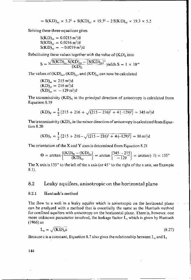
= S(KD),, x 5.22 + S(KD),, x 19.32 - 2 S(KD),, x 19.3 x 5.2
The orientation of the X and Y axes is determined from Equation 8.21
The X axis is 135 O to the left of the x axis (or 45 O to the right of the x axis, see Example 8.1).
8.2 Leaky aquifers, anisotropic on the horizontal plane
8.2.1 Hantush's method
The flow to a well in a leaky aquifer which is anisotropic on the horizontal plane can be analyzed with a method that is essentially the same as the Hantush method for confined aquifers with anisotropy on the horizontal plane. There is, however, one more unknown parameter involved, the leakage factor L, which is given by Hantush (1 966) as
L" = JE (8.27)
Because c is a constant, Equation 8.7 also gives the relationship between L, and L,
144
2 = cos2(@ + a,) + m sin2(@ + a,) cos2@ + m sin2@ an = - I (8.28)
I The Hantush method can be applied if the following assumptions and conditions are
- The assumptions listed at the beginning of Chapter 3, with the exception of the I satisfied:
first and third assumptions, which are replaced by: The aquifer is leaky; The aquifer is homogeneous, anisotropic on the horizontal plane, and of uniform thickness over the area influenced by the pumping test.
The following condition is added: - The flow to the well is in an unsteady state.
Procedure 8.5 This procedure is the same as Procedures 8.1 and 8.2 (the Hantush method for confined aquifers with anisotropy on the horizontal plane), except that, in the first step of Proce- dure 8.5, the methods for leaky isotropic aquifers (Section 4.2) are used to determine values for (KD),, S/(KD),, and L,. Further, Equation 8.28 is used instead of Equation 8.7.
I 8.3 Confined aquifers, anisotropic on the vertical plane
I The flow towards a well that completely penetrates a confined, horizontally stratified aquifer takes place essentially in planes parallel to the aquifer’s bedding planes. Even if the hydraulic conductivities vary appreciably in horizontal and vertical directions, the effect of any anisotropy on the vertical plane may not be of any great significance.
In thick aquifers, however, wells usually penetrate only a portion of the aquifer. The flow to such partially penetrating wells is not horizontal, but three-dimensional, i.e. the flow has significant vertical components, at least in the vicinity of the well, where most observations of the drawdown are made. In aquifers with very pronounced anisotropy on the vertical plane, the yield of partially penetrating wells may be appre- ciably smaller than that of similar wells in isotropic aquifers.
8.3.1 Weeks’s method
For large values of pumping time (t > DS/2KV) in a well that partially penetrates a confined aquifer, Hantush (1961a) developed a solution for the drawdown. After modification for the influence of anisotropy on the vertical plane, this equation becomes (Hantush 1964; Weeks 1969)
(8.29)
where W(u) = Theis well function
145
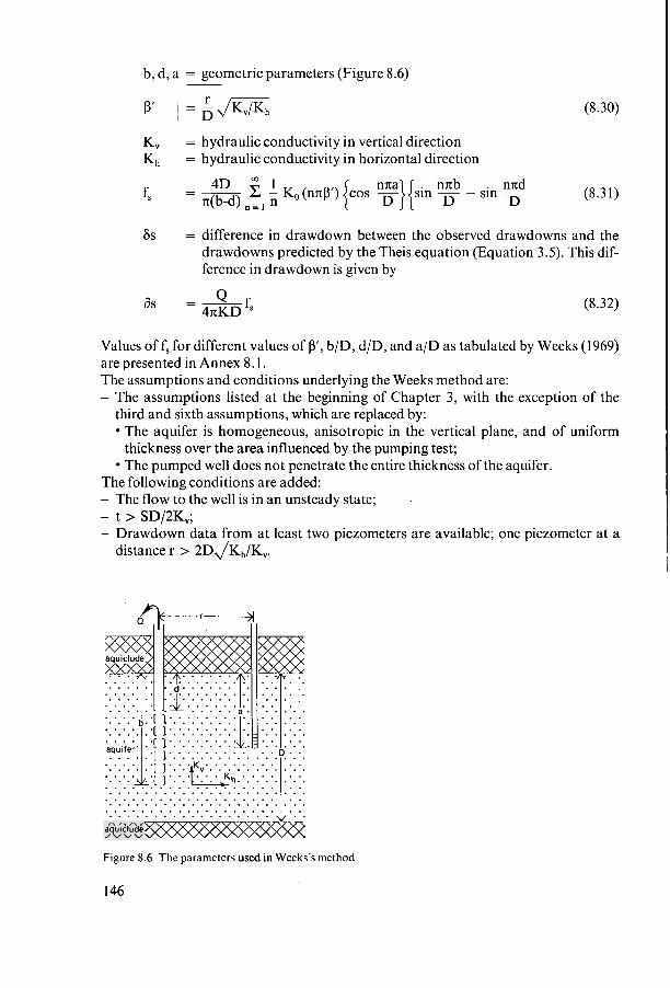
b, d, a = geometric parameters (Figure 8.6)
P’ ~ = g X h
K, K,
= hydraulic conductivity in vertical direction = hydraulic conductivity in horizontal direction
4D 1 { n;}{ . n;b . nnd - K,(nnp’) cos - sin ~ - sin ~
-- - .n(b-d) ” = I n D fs
(8.30)
(8.31)
6s = difference in drawdown between the observed draw-Dwns and the drawdowns predicted by the Theis equation (Equation 3.5). This dif- ference in drawdown is given by
Q 8s = - 4nKD fs (8.32)
Values off, for different values of P’, b/D, d/D, and a/D as tabulated by Weeks (1969) are presented in Annex 8. I . The assumptions and conditions underlying the Weeks method are: - The assumptions listed at the beginning of Chapter 3, with the exception of the
third and sixth assumptions, which are replaced by: The aquifer is homogeneous, anisotropic in the vertical plane, and of uniform
The pumped well does not penetrate the entire thickness of the aquifer. thickness over the area influenced by the pumping test;
The following conditions are added: - The flow to the well is in an unsteady state;
- Drawdown data from at least two piezometers are available; one piezometer at a - t > SD/2K,;
Procedure 8.6 - Apply one of the methods for confined, fully penetrated, isotropic a uifers (Section
3.2) to the observed drawdown data of Piezometer 1 at r > 2D,/&, and deter- mine the values of KhD and s;
- For Piezometer 2 at r < 2 D , / w , plot the observed drawdown s versus t on semi-log paper (t on logarithmic scale). Draw a straight line through the late-time data;
- Knowing Q, K,D, S, and r, calculate, for different values o f t , the values of s that would have occurred in Piezometer 2 if the pumped well had been fully penetrating;
use Equation 3.5, s = - W(u), and Annex 3.1; 4nKD - Plot these calculated values of s versus t on the same sheet of semi-log paper as
used for the observed time-drawdown plot. Draw a straight line through the late- time data. The straight lines of the two data plots should be parallel;
- Determine the vertical distance 6s between the two straight lines; - Knowing 6s, Q, and KhD, calculate f, from Equation 8.32; - Knowing f,, use Annex 8.1 to determine the value of p’ for the values of b/D, d/D,
and a/D nearest to the observed values for Piezometer 2; - Knowing p’ and r/D for Piezometer 2, calculate K,/K, from Equation 8.30; - Knowing K,/Kh, KhD, and D, calculate K, and K,.
Remarks - Instead of determining KhD and S with data from a piezometer at r > 2D,/K,/Kv
from the partially penetrating well, one can, of course, also obtain these valies from the data of a separate pumping test conducted in the same aquifer with a fully pene- trating well;
- Whether 8s will have a positive or a negative value depends on the location of Piez- ometer 2 relative to that of the screen of the partially penetrating well. When both are located at the same depth in the aquifer, the observed drawdown in Piezometer 2 will be greater than the theoretical drawdown for a fully penetrating well and consequently, 8s will have a positive value.
8.4 Leaky aquifers, anisotropic on the vertical plane
8.4.1 Weeks’s method
For large values of pumping time (t > DS/2KV) in a well that partially penetrates a leaky aquifer with anisotropy on the vertical plane, the drawdown response is given by (Hantush 1964; Weeks 1969)
where
W(u,r/L) = Walton’s well function
147
f,, p‘, b, d, a, and 6s are as defined in Section 8.3.1. A procedure similar to Procedure 8.6 can be applied to leaky aquifers.
The following assumptions and conditions should be satisfied: - The assumptions listed at the beginning of Chapter 3, with the exception of the
first, third, and sixth assumptions, which are replaced by: The aquifer is leaky; The aquifer is homogeneous, anisotropic on the vertical plane, and of uniform
The pumped well does not penetrate the entire thickness of the aquifer. thickness over the area influenced by the pumping test;
The following conditions are added: - The aquitard is incompressible; - The flow to the well is in unsteady state;
- Drawdown data from at least two piezometers are available; one piezometer at a - t > SD/2K,;
distancer > 2 D , / m .
Procedure 8.7 - Apply one of the methods for leaky, fully penetrated, isotropic aquifers (Sec-
tions 4.2 1 4 2 2, or 4.2.3) to the observed drawdown data of Piezometer 1 at r > 2 D , , / E , and determine the values of KhD, S, and L;
- For Piezometer 2 at r < 2 D , / a , plot the observed drawdown s versus t on log-log paper;
- Knowing Q, KhD, S , L, and r, calculate for different values o f t the values of s that would have occurred in Piezometer 2 if the pumped well had been fully penetrat- ing; use Equation 4.6
and Annex 4.2; - Plot these calculated values of s versus t on the same sheet of log-log paper as used
for the observed time-drawdown plot. The late-time parts of the data curves should be parallel;
- Determine the vertical distance 6s between the late-time parallel parts of the data curves;
- Knowing 6s, Q, and KhD, calculate f, from Equation 8.32; - Knowing f,, use Annex 8.1 to determine the value of 0’ for the values of b/D, d/D
and a/D nearest to the observed values for Piezometer 2; - Knowing p’ and r/D for Piezometer 2, calculate KJK, from Equation 8.30; - Knowing K&, KhD, and D, calculate Kh and K,.
8.5 Unconfined aquifers, anisotropic on the vertical plane
The flow to a well that pumps an unconfined aquifer is considered to be three-dimen- sional during the time that the delayed watertable response prevails (see Chapter 5). As three-dimensional flow is affected by anisotropy on the vertical plane, one of the
148
standard methods for unconfined aquifers already takes this anisotropy into account: Neuman’s curve-fitting method (Section 5. I . 1).
Apart from that standard method, there are other methods that take anisotropy on the vertical plane into account. They can be used when the well is partially penetrat- ing. They are Streltsova’s curve-fitting method (Section 10.4. I), Neuman’s curve-fit- ting method (Section 10.4.2), and Boulton-Streltsova’s curve-fitting method (Section 11.2.1).