8 File Processing and External Sorting In earlier chapters we discussed basic data structures and algorithms that operate on data stored in main memory. Sometimes the application at hand requires that large amounts of data be stored and processed, so much data that they cannot all fit into main memory. In that case, the data must reside on disk and be brought into main memory selectively for processing. You probably already realize that main memory access is much faster than ac- cess to data stored on disk or other storage devices. In fact, the relative difference in access times is so great that efficient disk-based programs require a different ap- proach to algorithm design than most programmers are used to. As a result, many programmers do a poor job when it comes to file processing applications. This chapter presents the fundamental issues relating to the design of algo- rithms and data structures for disk-based applications. We begin with a descrip- tion of the significant differences between primary memory and secondary storage. Section 8.2 discusses the physical aspects of disk drives. Section 8.3 presents basic methods for managing buffer pools. Buffer pools will be used several times in the following chapters. Section 8.4 discusses the C ++ model for random access to data stored on disk. Sections 8.5 to 8.8 discuss the basic principles of sorting collections of records too large to fit in main memory. 8.1 Primary versus Secondary Storage Computer storage devices are typically classified into primary or main memory and secondary or peripheral storage. Primary memory usually refers to Random Access Memory (RAM), while secondary storage refers to devices such as hard 271
Transcript
8
File Processing and ExternalSorting
In earlier chapters we discussed basic data structures and algorithms that operateon data stored in main memory. Sometimes the application at hand requires thatlarge amounts of data be stored and processed, so much data that they cannot all fitinto main memory. In that case, the data must reside on disk and be brought intomain memory selectively for processing.
You probably already realize that main memory access is much faster than ac-cess to data stored on disk or other storage devices. In fact, the relative differencein access times is so great that efficient disk-based programs require a different ap-proach to algorithm design than most programmers are used to. As a result, manyprogrammers do a poor job when it comes to file processing applications.
This chapter presents the fundamental issues relating to the design of algo-rithms and data structures for disk-based applications. We begin with a descrip-tion of the significant differences between primary memory and secondary storage.Section 8.2 discusses the physical aspects of disk drives. Section 8.3 presents basicmethods for managing buffer pools. Buffer pools will be used several times in thefollowing chapters. Section 8.4 discusses the C++ model for random access to datastored on disk. Sections 8.5 to 8.8 discuss the basic principles of sorting collectionsof records too large to fit in main memory.
8.1 Primary versus Secondary Storage
Computer storage devices are typically classified into primary or main memoryand secondary or peripheral storage. Primary memory usually refers to RandomAccess Memory (RAM), while secondary storage refers to devices such as hard
271
272 Chap. 8 File Processing and External Sorting
Medium Early 1996 Mid-1997 Early 2000RAM $45.00 7.00 1.50Disk 0.25 0.10 0.01Floppy 0.50 0.36 0.25Tape 0.03 0.01 0.001
Figure 8.1 Price comparison table for some writeable electronic data storagemedia in common use. Prices are in US Dollars/MB.
disk drives, floppy disk drives, and tape drives. Primary memory also includescache and video memories, but we will ignore them since their existence does notaffect the principal differences between primary and secondary memory.
Along with a faster CPU, every new model of computer seems to come withmore main memory. As memory size continues to increase, is it possible that rela-tively slow disk storage will be unnecessary? Probably not, since the desire to storeand process larger files grows at least as fast as main memory size. Prices for bothmain memory and peripheral storage devices have dropped dramatically in recentyears, as demonstrated by Figure 8.1. However, the cost for disk drive storage permegabyte is about two orders of magnitude less than RAM and has been for manyyears. Floppy disks used to be considerably cheaper per megabyte than hard diskdrives, but now their price per megabyte is actually greater. Filling in the gap be-tween hard drives and floppy disks are removable drives such a Zip drives, whoseprice per storage unit is about an order of magnitude greater than that of a fixed diskdrive. Magnetic tape is perhaps an order of magnitude cheaper than disk. Opticalstorage such as CD-ROMs also provide cheap storage but are usually sold basedon their information content rather than their storage capacity. Thus, they are notincluded in Figure 8.1.
Secondary storage devices have at least two other advantages over RAM mem-ory. Perhaps most importantly, disk and tape files are persistent, meaning thatthey are not erased from disk and tape when the power is turned off. In contrast,RAM used for main memory is usually volatile – all information is lost with thepower. A second advantage is that floppy disks, CD-ROMs, and magnetic tape caneasily be transferred between computers. This provides a convenient way to takeinformation from one computer to another.
In exchange for reduced storage costs, persistence, and portability, secondarystorage devices pay a penalty in terms of increased access time. While not allaccesses to disk take the same amount of time (more on this later), the typical timerequired to access a byte of storage from a disk drive in early 2000 is around 9 ms(i.e., 9 thousandths of a second). This may not seem slow, but compared to the time
Sec. 8.1 Primary versus Secondary Storage 273
required to access a byte from main memory, this is fantastically slow. Access timefrom standard personal computer RAM in early 2000 is about 60 or 70 nanoseconds(i.e., 60 or 70 billionths of a second). Thus, the time to access a byte of data froma disk drive is about five to six orders of magnitude greater than that required toaccess a byte from main memory. While disk drive and RAM access times areboth decreasing, they have done so at roughly the same rate. Fifteen years agothe relative speeds were about the same as they are today, in that the difference inaccess time between RAM and a disk drive has remained in the range between afactor of 100,000 and 1,000,000.
To gain some intuition for the significance of this speed difference, consider thetime that it might take for you to look up the entry for disk drives in the index ofthis book, and then turn to the appropriate page. Call this your “primary memory”access time. If it takes you about 20 seconds to perform this access, then an accesstaking 100,000 times longer would require a bit less than a month.
It is interesting to note that while processing speeds have increased dramat-ically, and hardware prices have dropped dramatically, disk and memory accesstimes have improved by less than a factor of two over the past ten years. However,the situation is really much better than that modest speedup would suggest. Dur-ing the same time period, the size of both disk and main memory has increased byabout two orders of magnitude. Thus, the access times have actually decreased inthe face of a massive increase in the density of these storage devices.
Due to the relatively slow access time for data on disk as compared to mainmemory, great care is required to create efficient applications that process disk-based information. The million-to-one ratio of disk access time versus main mem-ory access time makes the following rule of paramount importance when designingdisk-based applications:
Minimize the number of disk accesses!
There are generally two approaches to minimizing disk accesses. The first isto arrange information so that if you do access data from secondary memory, youwill get what you need in as few accesses as possible, and preferably on the firstaccess. File structure is the term used for a data structure that organizes datastored in secondary memory. File structures should be organized so as to minimizethe required number of disk accesses. The other way to minimize disk accesses isto arrange information so that each disk access retrieves additional data that canbe used to minimize the need for future accesses, that is, to guess accurately whatinformation will be needed later and retrieve it from disk now, if this can be donecheaply. As you shall see, there is little or no difference in the time required to
274 Chap. 8 File Processing and External Sorting
read several hundred contiguous bytes from disk or tape as compared to readingone byte, so this technique is indeed practical.
One way to minimize disk accesses is to compress the information stored ondisk. Section 3.9 discusses the space/time tradeoff in which space requirements canbe reduced if you are willing to sacrifice time. However, the disk-based space/timetradeoff principle stated that the smaller you can make your disk storage require-ments, the faster your program will run. This is because the time to read informa-tion from disk is enormous compared to computation time, so almost any amountof additional computation to unpack the data is going to be less than the disk readtime saved by reducing the storage requirements. This is precisely what happenswhen files are compressed. CPU time is required to uncompress information, butthis time is likely to be much less than the time saved by reducing the number ofbytes read from disk. Current file compression programs are not designed to allowrandom access to parts of a compressed file, so the disk-based space/time tradeoffprinciple cannot easily be taken advantage of in normal processing using commer-cial disk compression utilities. However, in the future disk drive controllers mayautomatically compress and decompress files stored on disk, thus taking advantageof the disk-based space/time tradeoff principle to save both space and time. Manycartridge tape drives today automatically compress and decompress informationduring I/O.
8.2 Disk Drives
A C++ programmer views a random access file stored on disk as a contiguousseries of bytes, with those bytes possibly combining to form data records. Thisis called the logical file. The physical file actually stored on disk is usually nota contiguous series of bytes. It could well be in pieces spread all over the disk.The file manager, a part of the operating system, is responsible for taking requestsfor data from a logical file and mapping those requests to the physical locationof the data on disk. Likewise, when writing to a particular logical byte positionwith respect to the beginning of the file, this position must be converted by thefile manager into the corresponding physical location on the disk. To gain someappreciation for the the approximate time costs for these operations, you need tounderstand the physical structure and basic workings of a disk drive.
Disk drives are often referred to as direct access storage devices. This meansthat it takes roughly equal time to access any record in the file. This is in contrastto sequential access storage devices such as tape drives, which require the tapereader to process data from the beginning of the tape until the desired position has
Sec. 8.2 Disk Drives 275
(b)
Heads
Platters
(arm)Boom
(a)
TrackRead/Write
Spindle
Figure 8.2 (a) A typical disk drive arranged as a stack of platters. (b) One trackon a disk drive platter.
been reached. As you will see, the disk drive is only approximately direct access:At any given time, some records are more quickly accessible than others.
8.2.1 Disk Drive Architecture
A hard disk drive is composed of one or more round platters, stacked one on top ofanother and attached to a central spindle. Platters spin continuously at a constantrate, like a record on a phonograph. Each usable surface of each platter is assigned aread/write head or I/O head through which data are read or written, somewhat likethe arrangement of a phonograph player’s arm “reading” sound from a phonographrecord. Unlike a phonograph needle, the disk read/write head does not actuallytouch the surface of a hard disk. Instead, it remains slightly above the surface, andany contact during normal operation would damage the disk. This distance is verysmall, much smaller than the height of a dust particle. It can be likened to a 5000-kilometer airplane trip across the United States, with the plane flying at a height ofone meter! In contrast, the read/write head on a floppy disk drive is in contact withthe surface of the disk, which in part accounts for its relatively slow access time.
A hard disk drive typically has several platters and several read/write heads, asshown in Figure 8.2(a). Each head is attached to an arm, which connects to theboom. The boom moves all of the heads in or out together. When the heads are insome position over the platters, there are data on each platter directly accessible toeach head. The data on a single platter that are accessible to any one position ofthe head for that platter are collectively called a track, that is, all data on a platterthat are a fixed distance from the spindle, as shown in Figure 8.2(b). The collectionof all tracks that are a fixed distance from the spindle is called a cylinder. Thus, acylinder is all of the data that can be read when the arms are in a particular position.
276 Chap. 8 File Processing and External Sorting
IntersectorGaps
Sectors
Bits of Data
Figure 8.3 The organization of a disk platter. Dots indicate density of informa-tion.
Each track is subdivided into sectors. Between each sector there are intersec-tor gaps in which no data are stored. These gaps allow the read head to recognizethe end of a sector. Note that each sector contains the same amount of data. Sincethe outer tracks have greater length, they contain fewer bits per inch than do the in-ner tracks. Thus, about half of the potential storage space is wasted, since only theinnermost tracks are stored at the highest possible data density. This arrangementis illustrated by Figure 8.3.
In contrast to the physical layout of a hard disk, a CD-ROM (and some floppydisk configurations) consists of a single spiral track. Bits of information along thetrack are equally spaced, so the information density is the same at both the outer andinner portions of the track. To keep the information flow at a constant rate along thespiral, the drive must slow down the rate of disk spin as the I/O head moves towardthe center of the disk. This makes for a more complicated and slower mechanism.
Three separate steps take place when reading a particular byte or series of bytesof data from a hard disk. First, the I/O head moves so it is positioned over the trackcontaining the data. This movement is called a seek. Second, the sector containingthe data rotates to come under the head. When in use the disk is always spinning. Atthe time of this writing, typical disk spin rates are 3600, 5400, and 7200 rotationsper minute (rpm), with 3600 rpm being phased out. The time spent waiting for thedesired sector to come under the I/O head is called rotational delay or rotationallatency. The third step is the actual transfer (i.e., reading or writing) of data. Ittakes relatively little time to read information once the first byte is positioned under
Sec. 8.2 Disk Drives 277
Head Head
Rotation Rotation
8
2
3
45
6
7
1
4
5
8
6
7
3
2
1
(a) (b)
Figure 8.4 The organization of a disk drive track. (a) No interleaving of sectors.(b) Sectors arranged with an interleaving factor of three.
the I/O head, simply the amount of time required for it all to move under the head.In fact, disk drives are designed not to read one byte of data, but rather to read anentire sector of data at each request. Thus, a sector is the minimum amount of datathat can be read or written at one time.
After reading a sector of data, the computer must take time to process it. Whileprocessing takes place, the disk continues to rotate. When reading several contigu-ous sectors of data at one time, this rotation creates a problem since the drive willread the first sector, process data, and find that the second sector has moved outfrom under the I/O head in the meantime. The disk must then rotate to bring thesecond sector under the I/O head.
Since each disk has fixed rotation rate and fixed processing time for one sectorof data, system designers can know how far the disk will rotate between the timewhen a sector is read and when the I/O head is ready for the next sector. Instead ofhaving the second logical sector physically adjacent to the first, it is better for thesecond logical sector to be at the position that will be under the I/O head when theI/O head is ready for it. Arranging data in this way is called interleaving, and thephysical distance between logically adjacent sectors is called the interleaving fac-tor. Figure 8.4(b) shows the sectors within one track arranged with an interleavingfactor of three. Sector 2 is separated from Sector 1 by Sectors 4 and 7. Reading anentire track will require three rotations of the disk from the time when Sector 1 firstmoves under the I/O head. During the first rotation, Sectors 1, 2, and 3 can be read.During the second rotation, Sectors 4, 5, and 6 can be read. Sectors 7 and 8 can beread during the third rotation.
278 Chap. 8 File Processing and External Sorting
Contrast reading the interleaved sectors of Figure 8.4(b) with the simple con-tiguous arrangement of Figure 8.4(a). After reading the first sector, and followingsome delay to process the information just read, the disk must rotate until Sector 2is once again under the I/O head, nearly a full rotation. Without interleaving, eightrotations of the disk are needed to read the entire track of Figure 8.4(a).
In general, it is desirable to keep all sectors for a file together on as few tracksas possible. This desire stems from two assumptions:
1. Seek time is slow (it is typically the most expensive part of an I/O operation),and
2. If one sector of the file is read, the next sector will probably soon be read.
Assumption (2) is called locality of reference, a concept that comes up frequentlyin computer science.
Contiguous sectors are often grouped to form a cluster.1 A cluster is the small-est unit of allocation for a file, so all files are a multiple of the cluster size. Thecluster size is determined by the operating system. The file manager keeps track ofwhich clusters make up each file.
In MS-DOS systems, there is a designated portion of the disk called the FileAllocation Table, which stores information about which sectors belong to whichfile. In contrast, UNIX does not use clusters. The smallest unit of file allocation andthe smallest unit that can be read/written is a sector, which in UNIX terminologyis called a block. UNIX maintains information about file organization in certainblocks called i-nodes.
A group of physically contiguous clusters from the same file is called an extent.Ideally, all clusters making up a file will be contiguous on the disk (i.e., the file willconsist of one extent), so as to minimize seek time required to access differentportions of the file. If the disk is nearly full when a file is created, there may not bean extent available that is large enough to hold the new file. Furthermore, if a filegrows, there may not be free space physically adjacent. Thus, a file may consist ofseveral extents widely spaced on the disk. The fuller the disk, and the more that fileson the disk change, the worse this file fragmentation (and the resulting seek time)becomes. File fragmentation leads to a noticeable degradation in performance asadditional seeks are required to access data.
Another type of problem arises when the file’s logical record size does notmatch the sector size. If the sector size is not a multiple of the record size (orvice versa), records will not fit evenly within a sector. For example, a sector might
1While the sectors of a cluster are logically contiguous, their physical layout on the disk may takeadvantage of interleaving to speed access. Whenever I refer to “contiguous” sectors in this chapter, beaware that this is contiguous in the logical sense and does not mean to preclude the use of interleaving.
Sec. 8.2 Disk Drives 279
Intersector Gap
DataSectorHeader Data
SectorSectorHeader
Sector
Intrasector Gap
Figure 8.5 An illustration of sector gaps within a track. Each sector begins witha sector header containing the sector address and an error detection code for thecontents of that sector. The sector header is followed by a small intrasector gap,followed in turn by the sector data. Each sector is separated from the next sectorby a larger intersector gap.
be 2048 bytes long, and a logical record 100 bytes. This leaves room to store20 records with 48 bytes left over. Either the extra space is wasted, or else recordsare allowed to cross sector boundaries. If a record crosses a sector boundary, twodisk accesses may be required to read it. If the space is left empty instead, suchwasted space is called internal fragmentation.
A second example of internal fragmentation occurs at cluster boundaries. Fileswhose size is not an even multiple of the cluster size must waste some space atthe end of the last cluster. The worst case will occur when file size modulo clustersize is one (for example, a file of 4097 bytes and a cluster of 4096 bytes). Thus,cluster size is a tradeoff between large files processed sequentially (where a largecluster size is desirable to minimize seeks) and small files (where small clusters aredesirable to minimize wasted storage).
Every disk drive organization requires that some disk space be used to organizethe sectors, clusters, and so forth. The layout of sectors within a track is illustratedby Figure 8.5. Typical information that must be stored on the disk itself includesthe File Allocation Table, sector headers that contain address marks and informa-tion about the condition (whether usable or not) for each sector, and gaps betweensectors. The sector header also contains error detection codes to help verify thatthe data have not been corrupted. This is why most disk drives have a “nominal”size that is greater than the actual amount of user data that can be stored on thedrive. A typical example might be a disk drive with a nominal size of 1044MBthat actually provides 1000MB of disk space after formatting. The difference is theamount of space required to organize the information on the disk. Additional spacewill be lost due to fragmentation.
280 Chap. 8 File Processing and External Sorting
8.2.2 Disk Access Costs
The primary cost when accessing information on disk is normally the seek time.This assumes of course that a seek is necessary. When reading a file in sequentialorder (if the sectors comprising the file are contiguous on disk), little seeking isnecessary. However, when accessing a random disk sector, seek time becomes thedominant cost for the data access. While the actual seek time is highly variable,depending on the distance between the track where the I/O head currently is andthe track where the head is moving to, we will consider only two numbers. Oneis the track-to-track cost, or the minimum time necessary to move from a track toan adjacent track. This is appropriate when you want to analyze access times forfiles that are well placed on the disk. The second number is the average seek timefor a random access. These two number are often provided by disk manufacturers.A typical example is the 16.8GB IBM Deskstar 16GP. The manufacturer’s specifi-cations indicate that the track-to-track time is 2.2 ms and the average seek time is9.5 ms.
For many years, typical rotation speed for disk drives was 3600 rpm, or one ro-tation every 16.7 ms. Newer disk drives have a rotation speed of 5400 or 7200 rpm.When reading a sector at random, you can expect that the disk will need to ro-tate halfway around to bring the desired sector under the I/O head, or 5.6 ms for a5400-rpm disk drive and 4.2 ms for a 7200-rpm disk drive.
Once under the I/O head, a sector of data can be transferred as fast as thatsector rotates under the head. If an entire track is to be read, then it will requireone rotation (8.3 ms at 7200 rpm) to move the full track under the head. Of course,when reading a full track of data, interleaving will affect the number of rotationsactually required. If only part of the track is to be read, then proportionately lesstime will be required. For example, if there are 256 sectors on the track and onesector is to be read, this will require a trivial amount of time (1/256 of a rotation).
Example 8.1 Assume that a disk drive has a total (nominal) capacity of16.8GB spread among 10 platters, yielding 1.68GB/platter. Each plattercontains 13,085 tracks and each track contains (after formating) 256 sec-tors of 512 bytes/sector. Track-to-track seek time is 2.2 ms and averageseek time for random access is 9.5 ms. Assume the operating system main-tains a cluster size of 8 sectors per cluster (4KB), yielding 32 clusters pertrack. The disk rotation rate is 5400 rpm. Based on this information we canestimate the cost for various file processing operations.
Assume that the interleaving factor is three. How many rotations ofthe disk will be required to read one track once the first sector of the track
Sec. 8.2 Disk Drives 281
is under the I/O head? The answer is three, since one third of the sectorswill be read during each rotation. How much time is required to read thetrack? Since it requires three rotations at 11.1 ms per rotation, the entiretime is 33.3 ms. Note that this ignores the time to seek to the track, and therotational latency while the first sector moves under the I/O head.
How long will it take to read a file of 1MB divided into 2048 sector-sized (512 byte) records? This file will be stored in 256 clusters, since eachcluster holds 8 sectors. The answer to the question depends in large measureon how the file is stored on the disk, that is, whether it is all together orbroken into multiple extents. We will calculate both cases to see how muchdifference this makes.
If the file is stored so as to fill all of the sectors of eight adjacent tracks,then the cost to read the first sector will be the time to seek to the firsttrack (assuming this requires a random seek), then a wait for the initialrotational delay, and then the time to read (requiring three rotations due tointerleaving). This requires
9.5 + 11.1/2 + 3 × 11.1 = 48.4 ms.
At this point, since we assume that the next seven tracks require only atrack-to-track seek since they are adjacent, each requires
2.2 + 11.1/2 + 3 × 11.1 = 41.1 ms.
The total time required is therefore
48.4ms + 7 × 41.1ms = 335.7ms.
If the file’s clusters are spread randomly across the disk, then we mustperform a seek for each cluster, followed by the time for rotational delay.At an interleaving factor of three, reading one cluster requires that the diskmake (3 ∗ 8)/256 of a rotation, for a total of 1 ms. Thus, the total timerequired is
256(9.5 + 11.1/2 + (3 ∗ 8)/256) ≈ 3877ms
or close to 4 seconds. This is much longer than the time required when thefile is all together on disk!
This example illustrates why it is important to keep disk files from be-coming fragmented, and why so-called “disk defragmenters” can speed upfile processing time. File fragmentation happens most commonly when thedisk is nearly full and the file manager must search for free space whenevera file is created or changed.
282 Chap. 8 File Processing and External Sorting
8.3 Buffers and Buffer Pools
Given the specifications of the disk drive from Example 8.1, we find that it takesabout 9.5+11.1/2+3×11.1 = 48.4 ms to read one track of data on average whenthe interleaving factor is 3. Even if interleaving were unnecessary, it would stillrequire 9.5 + 11.1/2 + 11.1 = 26.2 ms. It takes about 9.5 + 11.1/2 + (1/256) ×11.1 = 15.1 ms on average to read a single sector of data. This is a good savings(slightly over one third the time for an interleaving factor of 3), but less than 1%of the data on the track are read. If we want to read only a single byte, it wouldsave us less than 0.05 ms over the time required to read an entire sector. This is aninsignificant savings in time when we consider the cost of seeking and rotationaldelay. For this reason, nearly all disk drives automatically read or write an entiresector’s worth of information whenever the disk is accessed, even when only onebyte of information is requested.
Once a sector is read, its information is stored in main memory. This is knownas buffering or caching the information. If the next disk request is to that samesector, then it is not necessary to read from disk again; the information is alreadystored in main memory. Buffering is an example of one method for minimizing diskaccesses stated at the beginning of the chapter: Bring off additional informationfrom disk to satisfy future requests. If information from files were accessed atrandom, then the chance that two consecutive disk requests are to the same sectorwould be low. However, in practice most disk requests are close to the location (inthe logical file at least) of the previous request. This means that the probability ofthe next request “hitting the cache” is much higher than chance would indicate.
This principle explains one reason why average access times for new disk drivesare lower than in the past. Not only is the hardware faster, but information is alsonow stored using better algorithms and larger caches that minimize the number oftimes information needs to be fetched from disk. This same concept is also used tostore parts of programs in faster memory within the CPU, the so-called CPU cachethat is prevalent in modern microprocessors.
Sector-level buffering is normally provided by the operating system and is of-ten built directly into the disk drive controller hardware. Most operating systemsmaintain at least two buffers, one for input and one for output. Consider whatwould happen if there were only one buffer during a byte-by-byte copy operation.The sector containing the first byte would be read into the I/O buffer. The outputoperation would need to destroy the contents of the single I/O buffer to write thisbyte. Then the buffer would need to be filled again from disk for the second byte,only to be destroyed during output. The simple solution to this problem is to keepone buffer for input, and a second for output.
Sec. 8.3 Buffers and Buffer Pools 283
Most disk drive controllers operate independently from the CPU once an I/Orequest is received. This is useful since the CPU can typically execute millions ofinstructions during the time required for a single I/O operation. A technique thattakes maximum advantage of this microparallelism is double buffering. Imaginethat a file is being processed sequentially. While the first sector is being read, theCPU cannot process that information and so must wait or find something else to doin the meantime. Once the first sector is read, the CPU can start processing whilethe disk drive (in parallel) begins reading the second sector. If the time required forthe CPU to process a sector is approximately the same as the time required by thedisk controller to read a sector, it may be possible to keep the CPU continuouslyfed with data from the file. The same concept can also be applied to output, writingone sector to disk while the CPU is writing to a second output buffer in memory.Thus, in computers that support double buffering, it pays to have at least two inputbuffers and two output buffers available.
Caching information in memory is such a good idea that it is usually extendedto multiple buffers. The operating system or an application program may storemany buffers of information taken from some backing storage such as a disk file.This process of using buffers as an intermediary between a user and a disk file iscalled buffering the file. The information stored in a buffer is often called a page,and the collection of buffers is called a buffer pool. The goal of the buffer poolis to increase the amount of information stored in memory in hopes of increasingthe likelihood that new information requests can be satisfied from the buffer poolrather than requiring new information to be read from disk.
As long as there is an unused buffer available in the buffer pool, new informa-tion can be read in from disk on demand. When an application continues to readnew information from disk, eventually all of the buffers in the buffer pool will be-come full. Once this happens, some decision must be made about what informationin the buffer pool will be sacrificed to make room for newly requested information.
When replacing information contained in the buffer pool, the goal is to selecta buffer that has “unnecessary” information, that is, that information least likely tobe requested again. Since the buffer pool cannot know for certain what the patternof future requests will look like, a decision based on some heuristic, or best guess,must be used. There are several approaches to making this decision.
One heuristic is “first-in, first-out” (FIFO). This scheme simply orders thebuffers in a queue. The buffer at the front of the queue is used next to store newinformation and then placed at the end of the queue. In this way, the buffer to bereplaced is the one that has held its information the longest, in hopes that this in-formation is no longer needed. This is a reasonable assumption when processing
284 Chap. 8 File Processing and External Sorting
moves along the file at some steady pace in roughly sequential order. However,many programs work with certain key pieces of information over and over again,and the importance of information has little to do with how long ago the informa-tion was first accessed. Typically it is more important to know how many times theinformation has been accessed, or how recently the information was last accessed.
Another approach is called “least frequently used” (LFU). LFU tracks the num-ber of accesses to each buffer in the buffer pool. When a buffer must be reused, thebuffer that has been accessed the fewest number of times is considered to containthe “least important” information, and so it is used next. LFU, while it seems in-tuitively reasonable, has many drawbacks. First, it is necessary to store and updateaccess counts for each buffer. Second, what was referenced many times in the pastmay now be irrelevant. Thus, some time mechanism where counts “expire” is oftendesirable. This also avoids the problem of buffers that slowly build up big countsbecause they get used just often enough to avoid being replaced (unless counts aremaintained for all sectors ever read, not just the sectors currently in the buffer pool).
The third approach is called “least recently used” (LRU). LRU simply keeps thebuffers in a linked list. Whenever information in a buffer is accessed, this buffer isbrought to the front of the list. When new information must be read, the buffer atthe back of the list (the one least recently used) is taken and its “old” informationis either discarded or written to disk, as appropriate. This is an easily implementedapproximation to LFU and is the method of choice for managing buffer pools unlessspecial knowledge about information access patterns for an application suggests aspecial-purpose buffer management scheme.
Many operating systems support virtual memory. Virtual memory is a tech-nique that allows the programmer to pretend that there is more main memory thanactually exists. This is done by means of a buffer pool reading blocks from disk.The disk stores the complete contents of the virtual memory; blocks are read intomain memory as demanded by memory accesses. Naturally, programs using virtualmemory techniques are slower than programs whose data are stored completely inmain memory. The advantage is reduced programmer effort since a good virtualmemory system provides the appearance of larger main memory without modify-ing the program. Figure 8.6 illustrates the concept of virtual memory.
When implementing buffer pools, there are two basic approaches that can betaken regarding the transfer of information between the user of the buffer pool andthe buffer pool class itself. The first approach is to pass “messages” between thetwo. This approach is illustrated by the following abstract class:
Sec. 8.3 Buffers and Buffer Pools 285
(on disk)Physical Memory
(in main memory)
2
3
4
5
6
7
8
9
8
3
5
0
1 7
1
Virtual Memory
Figure 8.6 An illustration of virtual memory. The complete collection of in-formation resides on disk (physical memory). Those sectors recently accessedare held in main memory (virtual memory). In this example, copies of Sectors 1,7, 5, 3, and 8 from physical memory are currently stored in the virtual memory.If a memory access to Sector 9 is received, one of the sectors currently in mainmemory must be replaced.
class BufferPool {public:
// Insert from space sz bytes begining at position pos// of the buffered storevirtual void insert(void* space, int sz, int pos) = 0;// Put into space sz bytes beginning at position pos// of the buffered storevirtual void getbytes(void* space, int sz, int pos) = 0;
};
This simple class provides an interface with two functions, insert and getbytes.The information is passed between the buffer pool user and the buffer pool throughthe space parameter. This is storage space, at least sz bytes long, which thebuffer pool can take information from (the insert function) or put informationinto (the getbytes function). Parameter pos indicates where in the buffer pool’sstorage space the information will be placed.
The alternative approach is to have the buffer pool provide to the user a directpointer to a buffer that contains the necessary information. Such an interface mightlook as follows:
286 Chap. 8 File Processing and External Sorting
class BufferPool {public:
// Return pointer to the requested blockvirtual void* getblock(int block) = 0;// Set the dirty bit for buffer buffvirtual void dirtyblock(int block) = 0;// Tell the size of a buffervirtual int blocksize() = 0;
};
In this approach, the user of the buffer pool is made aware that the storagespace is divided into blocks of a given size, where each block is the size of a buffer.The user requests specific blocks from the buffer pool, with a pointer to the bufferholding the requested block being returned to the user. The user may then readfrom or write to this space. If the user writes to the space, the buffer pool must beinformed of this fact. The reason is that, when a given block is to be removed fromthe buffer pool, the contents of that block must be written to the backing storage ifit has been modified. If the block has not been modified, then it is unnecessary towrite it out.
A further problem with the second approach is the risk of stale pointers. Whenthe buffer pool user is given a pointer to some buffer space at time T1, that pointerdoes indeed refer to the desired data at that time. If further requests are made tothe buffer pool, it is possible that the data in any given buffer will be removed andreplaced with new data. If the buffer pool user at a later time T2 then refers to thedata refered to by the pointer given at time T1, it is possible that the data are nolonger valid because the buffer contents have been replaced in the meantime. Thusthe pointer into the buffer pool’s memory has become “stale.” To guarantee that apointer is not stale, it should not be used if intervening requests to the buffer poolhave taken place.
Clearly, the second approach places many obligations on the user of the bufferpool. These obligations include knowing the size of a block, not corrupting thebuffer pool’s storage space, informing the buffer pool when a block has been mod-ified, and avoiding use of stale pointers. So many obligations make this approachprone to error. The advantage is that there is no need to do an extra copy step whengetting information from the user to the buffer. If the size of the records storedis small, this is not an important consideration. If the size of the records is large(especially if the record size and the buffer size are the same, as typically is thecase when implementing B-trees, see Section 10.5), then this efficiency issue maybecome important. Note however that the in-memory copy time will always be farless than the time required to write the contents of a buffer to disk. For applica-
Sec. 8.4 The Programmer’s View of Files 287
tions where disk I/O is the bottleneck for the program, even the time to copy lots ofinformation between the buffer pool user and the buffer may be inconsequential.
You should note that the implementations for class BufferPool above arenot templates. Instead, the space parameter and the buffer pointer are declared tobe void*. When a class is a template, that means that the record type is arbitrary,but that the class knows what the record type is. In contrast, using a void* pointerfor the space means that not only is the record type arbitrary, but also the bufferpool does not even know what the user’s record type is. In fact, a given buffer poolmight have many users who store many types of records.
Another thing to note about the buffer pool is that the user decides where a givenrecord will be stored but has no control over the precise mechanism by which dataare transfered to the backing storage. This is in contrast to the memory managerdescribed in Section 12.4 in which the user passes a record to the manager and hasno control at all over where the record is stored.
8.4 The Programmer’s View of Files
As stated earlier, the C++ programmer’s logical view of a random access file is asingle stream of bytes. Interaction with a file can be viewed as a communicationschannel for issuing one of three instructions: read bytes from the current position inthe file, write bytes to the current position in the file, and move the current positionwithin the file. You do not normally see how the bytes are stored in sectors, clusters,and so forth. The mapping from logical to physical addresses is done by the filesystem, and sector-level buffering is done automatically by the operating system.
When processing records in a disk file, the order of access can have a greateffect on I/O time. A random access procedure processes records in an orderindependent of their logical order within the file. Sequential access processesrecords in order of their logical appearance within the file. Sequential processingrequires less seek time if the physical layout of the disk file matches its logicallayout, as would be expected if the file were created on a disk with a high percentageof free space.
C++ provides several mechanisms for manipulating binary files. One of themost commonly used is the fstream class. Following are the primary fstreamclass member functions for manipulating information in random access disk files.These functions constitute an ADT for files.
• open: Open a file for processing.• read: Read some bytes from the current position in the file. The current
position moves forward as the bytes are read.
288 Chap. 8 File Processing and External Sorting
• write: Write some bytes at the current position in the file (overwriting thebytes already at that position). The current position moves forward as thebytes are written.
• seekg and seekp: Move the current position in the file. This allows bytesat arbitrary places within the file to be read or written. There are actually two“current” positions: one for reading and one for writing. Function seekgchanges the “get” or read position, while function seekp changes the “put”or write position.
• close: Close a file at the end of processing.
8.5 External Sorting
We now consider the problem of sorting collections of records too large to fit inmain memory. Since the records must reside in peripheral or external memory, suchsorting methods are called external sorts in contrast to the internal sorts discussedin Chapter 7. Sorting large collections of records is central to many applications,such as processing payrolls and other large business databases. As a consequence,many external sorting algorithms have been devised. Years ago, sorting algorithmdesigners sought to optimize the use of specific hardware configurations, such asmultiple tape or disk drives. Most computing today is done on personal computersand low-end workstations with relatively powerful CPUs, but only one or at mosttwo disk drives. The techniques presented here are geared toward optimized pro-cessing on a single disk drive. This approach allows us to cover the most importantissues in external sorting while skipping many less important machine-dependentdetails. Readers who have a need to implement efficient external sorting algorithmsthat take advantage of more sophisticated hardware configurations should consultthe references in Section 8.9.
When a collection of records is too large to fit in main memory, the only prac-tical way to sort it is to read some records from disk, do some rearranging, thenwrite them back to disk. This process is repeated until the file is sorted, with eachrecord read perhaps many times. Armed with the basic knowledge about disk drivespresented in Section 8.2, it should come as no surprise that the primary goal of anexternal sorting algorithm is to minimize the amount of information that must beread from or written to disk. A certain amount of additional CPU processing canprofitably be traded for reduced disk access.
Before discussing external sorting techniques, consider again the basic modelfor accessing information from disk. The file to be sorted is viewed by the pro-grammer as a sequential series of fixed-size blocks. Assume (for simplicity) that
Sec. 8.5 External Sorting 289
each block contains the same number of fixed-size data records. Depending onthe application, a record may be only a few bytes – composed of little or nothingmore than the key – or may be hundreds of bytes with a relatively small key field.Records are assumed not to cross block boundaries. These assumptions can berelaxed for special-purpose sorting applications, but ignoring such complicationsmakes the principles clearer.
As explained in Section 8.2, a sector is the basic unit of I/O. In other words, alldisk reads and writes are for a single, complete sector. Sector sizes are typicallya power of two, in the range 1K to 16K bytes, depending on the operating systemand the size and speed of the disk drive. The block size used for external sortingalgorithms should be equal to or a multiple of the sector size.
Under this model, a sorting algorithm reads a block of data into a buffer in mainmemory, performs some processing on it, and at some future time writes it back todisk. From Section 8.1 we see that reading or writing a block from disk takes onthe order of one million times longer than a memory access. Based on this fact, wecan reasonably expect that the records contained in a single block can be sorted byan internal sorting algorithm such as Quicksort in less time than is required to reador write the block.
Under good conditions, reading from a file in sequential order is more efficientthan reading blocks in random order. Given the significant impact of seek timeon disk access, it may seem obvious that sequential processing is faster. However,it is important to understand precisely under what circumstances sequential fileprocessing is actually faster than random access, since it affects our approach todesigning an external sorting algorithm.
Efficient sequential access relies on seek time being kept to a minimum. Thefirst requirement is that the blocks making up a file are in fact stored on disk insequential order and close together, preferably filling a small number of contiguoustracks. At the very least, the number of extents making up the file should be small.Users typically do not have much control over the layout of their file on disk, butwriting a file all at once in sequential order to a disk drive with a high percentageof free space increases the likelihood of such an arrangement.
The second requirement is that the disk drive’s I/O head remain positionedover the file throughout sequential processing. This will not happen if there iscompetition of any kind for the I/O head. For example, on a multi-user timesharedcomputer the sorting process may compete for the I/O head with the process ofanother user. Even when the sorting process has sole control of the I/O head, itis still likely that sequential processing will not be efficient. Imagine the situationwhere all processing is done on a single disk drive, with the typical arrangement
290 Chap. 8 File Processing and External Sorting
of a single bank of read/write heads that move together over a stack of platters. Ifthe sorting process involves reading from an input file, alternated with writing to anoutput file, then the I/O head will continuously seek between the input file and theoutput file. Similarly, if two input files are being processed simultaneously (suchas during a merge process), then the I/O head will continuously seek between thesetwo files.
The moral is that, with a single disk drive, there often is no such thing as effi-cient, sequential processing of a data file. Thus, a sorting algorithm may be moreefficient if it performs a smaller number of non-sequential disk operations ratherthan a larger number of logically sequential disk operations that require a largenumber of seeks in practice.
As mentioned previously, the record size may be quite large compared to thesize of the key. For example, payroll entries for a large business may each storehundreds of bytes of information including the name, ID, address, and job title foreach employee. The sort key may be the ID number, requiring only a few bytes.The simplest sorting algorithm may be to process such records as a whole, readingthe entire record whenever it is processed. However, this will greatly increase theamount of I/O required, since only a relatively few records will fit into a single diskblock. Another alternative is to do a key sort. Under this method, the keys areall read and stored together in an index file, where each key is stored along witha pointer indicating the position of the corresponding record in the original datafile. The key and pointer combination should be substantially smaller than the sizeof the original record; thus, the index file will be much smaller than the completedata file. The index file will then be sorted, requiring much less I/O since the indexrecords are smaller than the complete records.
Once the index file is sorted, it is possible to reorder the records in the originaldatabase file. This is typically not done for two reasons. First, reading the recordsin sorted order from the record file requires a random access for each record. Thiscan take a substantial amount of time and is only of value if the complete collectionof records needs to be viewed or processed in sorted order (as opposed to a searchfor selected records). Second, database systems typically allow searches to be doneon multiple keys. In other words, today’s processing may be done in order of IDnumbers. Tomorrow, the boss may want information sorted by salary. Thus, theremay be no single “sorted” order for the full record. Instead, multiple index filesare often maintained, one for each sort key. These ideas are explored further inChapter 10.
Sec. 8.6 Simple Approaches to External Sorting 291
8.6 Simple Approaches to External Sorting
If your operating system supports virtual memory, the simplest “external” sort isto read the entire file into virtual memory and run an internal sorting method suchas Quicksort. This approach allows the virtual memory manager to use its normalbuffer pool mechanism to control disk accesses. Unfortunately, this may not alwaysbe a viable option. One potential drawback is that the size of virtual memory is usu-ally limited to something much smaller than the disk space available. Thus, yourinput file may not fit into virtual memory. Limited virtual memory can be over-come by adapting an internal sorting method to make use of your own buffer poolcombined with one of the buffer management techniques discussed in Section 8.3.
A more general problem with adapting an internal sorting algorithm to externalsorting is that it is not likely to be as efficient as designing a new algorithm withthe specific goal of minimizing disk fetches. Consider the simple adaptation ofQuicksort to external sorting. Quicksort begins by processing the entire array ofrecords, with the first partition step moving indices inward from the two ends. Thiscan be implemented efficiently using a buffer pool. However, the next step is toprocess each of the subarrays, followed by processing of sub-subarrays, and so on.As the subarrays get smaller, processing quickly approaches random access to thedisk drive. Even with maximum use of the buffer pool, Quicksort still must readand write each record log n times on average. You will soon see that it is possibleto do much better than this.
A better approach to external sorting can be derived from the Mergesort alg-orithm. The simplest form of Mergesort performs a series of sequential passes overthe records, merging larger and larger sublists on each pass. Thus, the first passmerges sublists of size 1 into sublists of size 2; the second pass merges the sublistsof size 2 into sublists of size 4; and so on. Such sorted sublists are called runs.Each sublist-merging pass copies the contents of the file to another file. Here is asketch of the algorithm, illustrated by Figure 8.7:
1. Split the original file into two equal-sized run files.2. Read one block from each run file into input buffers.3. Take the first record from each input buffer, and write them to an output run
buffer in sorted order.4. Take the next record from each input buffer, and write them to a second
output run buffer in sorted order.5. Repeat until finished, alternating output between the two output run buffers.
When an input block is exhausted, read the next block from the appropriateinput file. When an output run buffer is full, write it to the appropriate outputfile.
292 Chap. 8 File Processing and External Sorting
Runs of length 4Runs of length 2
36
15 23
20
13
14
15
2336 17 28
20 13 14 14
13
Runs of length 1
15
36 28
17 23
17 20
28
Figure 8.7 Illustration of a simple external Mergesort algorithm. Input recordsare divided equally among two input files. The first runs from each input file aremerged and placed in the first output file. The second runs from each input file aremerged and placed in the second output file. Merging alternates between the twooutput files until the input files are empty. The roles of input and output files arethen reversed, allowing the runlength to be doubled with each pass.
6. Repeat steps 2 through 5, using the original output files as input files. On thesecond pass, the first two records of each input run file are already in sortedorder. Thus, these two runs may be merged and output as a single run of fourelements.
7. Each pass through the run files provides larger and larger runs until only onerun remains.
This algorithm can easily take advantage of the double buffering techniquesdescribed in Section 8.3. Note that the various passes read the input run files se-quentially and write the output run files sequentially. For sequential processing anddouble buffering to be effective, however, it is necessary that there be a separateI/O head available for each file. This typically means that each of the input andoutput files must be on separate disk drives, requiring a total of four disk drives formaximum efficiency.
The external Mergesort algorithm just described requires that log n passes bemade to sort a file of n records. Thus, each record must be read from disk andwritten to disk log n times. The number of passes can be significantly reduced byobserving that it is not necessary to use Mergesort on small runs. A simple modifi-cation is to read in a block of data, sort it in memory (perhaps using Quicksort), andthen output it as a single sorted run. For example, assume that we have 4KB blocks,and 8-byte records each containing four bytes of data and a 4-byte key. Thus, eachblock contains 512 records. Standard Mergesort would require nine passes to gen-erate runs of 512 records, whereas processing each block as a unit can be done inone pass with an internal sort. These runs can then be merged by Mergesort. Stan-dard Mergesort requires eighteen passes to process 256K records. Using an internalsort to create initial runs of 512 records reduces this to one initial pass to create the
Sec. 8.7 Replacement Selection 293
runs and nine merge passes to put them all together, approximately half as manypasses.
We can extend this concept to improve performance even further. Availablemain memory is usually much more than one block in size. If we process largerinitial runs, then the number of passes required by Mergesort is further reduced.For example, most modern computers can make anywhere from half a megabyte toa few tens of megabytes of RAM available for processing. If all of this memory(excepting a small amount for buffers and local variables) is devoted to buildinginitial runs as large as possible, then quite large files can be processed in few passes.The next section presents a technique for producing large runs, typically twice aslarge as could fit directly into main memory.
Another way to reduce the number of passes required is to increase the numberof runs that are merged together during each pass. While the standard Mergesortalgorithm merges two runs at a time, there is no reason why merging needs to belimited in this way. Section 8.8 discusses the technique of multiway merging.
Over the years, many variants on external sorting have been presented. How-ever, most follow the same principles. In general, all good external sorting algo-rithms are based on the following two steps:
1. Break the file into large initial runs.2. Merge the runs together to form a single sorted file.
8.7 Replacement Selection
This section treats the problem of creating initial runs as large as possible from adisk file, assuming a fixed amount of RAM is available for processing. As men-tioned previously, a simple approach is to allocate as much RAM as possible to alarge array, fill this array from disk, and sort the array using Quicksort. Thus, ifthe size of memory available for the array is M records, then the input file can bebroken into initial runs of length M . A better approach is to use an algorithm calledreplacement selection that, on average, creates runs that are 2M records in length.Replacement selection is actually a slight variation on the Heapsort algorithm. Thefact that Heapsort is slower than Quicksort is irrelevant in this context since I/Otime will dominate the total running time of any reasonable external sorting alg-orithm.
Replacement selection views RAM as consisting of an array of size M in addi-tion to an input buffer and an output buffer. (Additional I/O buffers may be desir-able if the operating system supports double buffering, since replacement selectiondoes sequential processing on both its input and its output.) Imagine that the input
294 Chap. 8 File Processing and External Sorting
Input Buffer Output BufferFileInput
Run FileOutput
RAM
Figure 8.8 Overview of replacement selection. Input records are processed se-quentially. Initially RAM is filled with M records. As records are processed, theyare written to an output buffer. When this buffer becomes full, it is written to disk.Meanwhile, as replacement selection needs records, it reads them from the inputbuffer. Whenever this buffer becomes empty, the next block of records is readfrom disk.
and output files are streams of records. Replacement selection takes the next recordin sequential order from the input stream when needed, and outputs runs one recordat a time to the output stream. Buffering is used so that disk I/O is performed oneblock at a time. A block of records is initially read and held in the input buffer.Replacement selection removes records from the input buffer one at a time untilthe buffer is empty. At this point the next block of records is read in. Output to abuffer is similar: Once the buffer fills up it is written to disk as a unit. This processis illustrated by Figure 8.8.
Replacement selection works as follows. Assume that the main processing isdone in an array of size M records.
1. Fill the array from disk. Set LAST = M − 1.2. Build a min-heap. (Recall that a min-heap is defined such that the record at
each node has a key value less than the key values of its children.)3. Repeat until the array is empty:
(a) Send the record with the minimum key value (the root) to the outputbuffer.
(b) Let R be the next record in the input buffer. If R’s key value is greaterthan the key value just output ...
i. Then place R at the root.
ii. Else replace the root with the record in array position LAST, andplace R at position LAST. Set LAST = LAST − 1.
(c) Sift down the root to reorder the heap.
When the test at step 3(b) is successful, a new record is added to the heap,eventually to be output as part of the run. As long as records coming from the inputfile have key values greater than the last key value output to the run, they can be
Sec. 8.7 Replacement Selection 295
safely added to the heap. Records with smaller key values cannot be output as partof this run since they would not be in sorted order. Such values must be storedsomewhere for future processing as part of another run. However, since the heapwill shrink by one element in this case, there is now a free space where the lastelement of the heap used to be! Thus, replacement selection will slowly shrink theheap and at the same time use the discarded heap space to store records for the nextrun. Once the first run is complete (i.e., the heap becomes empty), the array will befilled with records ready to be processed for the second run. Figure 8.9 illustratespart of a run being created by replacement selection.
It should be clear that the minimum length of a run will be M records if the sizeof the heap is M , since at least those records originally in the heap will be part ofthe run. Under good conditions (e.g., if the input is sorted), then an arbitrarily longrun is possible – in fact, the entire file could be processed as one run. If conditionsare bad (e.g., if the input is reverse sorted), then runs of only size M result.
What is the expected length of a run generated by replacement selection? Itcan be deduced from an analogy called the snowplow argument. Imagine that asnowplow is going around a circular track during a heavy, but steady, snowstorm.After the plow has been around at least once, snow on the track must be as follows.Immediately behind the plow, the track is empty since it was just plowed. Thegreatest level of snow on the track is immediately in front of the plow, since thisis the place least recently plowed. At any instant, there is a certain amount ofsnow S on the track. Snow is constantly falling throughout the track at a steadyrate, with some snow falling “in front” of the plow and some “behind” the plow.(On a circular track, everything is actually “in front” of the plow, but Figure 8.10illustrates the idea.) During the next revolution of the plow, all snow S on the trackis removed, plus half of what falls. Since everything is assumed to be in steadystate, after one revolution S snow is still on the track, so 2S snow must fall duringa revolution, and 2S snow is removed during a revolution (leaving S snow behind).
At the beginning of replacement selection, nearly all values coming from theinput file are greater (i.e., “in front of the plow”) than the latest key value output forthis run, since the run’s initial key values should be small. As the run progresses,the latest key value output becomes greater and so new key values coming fromthe input file are more likely to be too small (i.e., “after the plow”); such recordsgo to the bottom of the array. The total length of the run is expected to be twicethe size of the array. Of course, this assumes that incoming key values are evenlydistributed within the key range (in terms of the snowplow analogy, we assume thatsnow falls evenly throughout the track). Sorted and reverse sorted inputs do notmeet this expectation and so change the length of the run.
296 Chap. 8 File Processing and External Sorting
Input Memory Output
16 12
29 16
14 19
21
25 29 56
31
14
35 25 31 21
40 29 56
21
40
56 402125
31
29
16
12
56 40
31
25
19
21
25 21 56
31
40
19
19
19
21
25
31
56 4029
14
Figure 8.9 Replacement selection example. After building the heap, rootvalue 12 is output and incoming value 16 replaces it. Value 16 is output next,replaced with incoming value 29. The heap is reordered, with 19 rising to theroot. Value 19 is output next. Incoming value 14 is too small for this run andis placed at end of the array, moving value 40 to the root. Reordering the heapresults in 21 rising to the root, which is output next.
Sec. 8.8 Multiway Merging 297
Existing snow
Future snow
Falling Snow
Snowplow Movement
Start time TFigure 8.10 Illustration of the snowplow analogy showing the action during onerevolution of the snowplow. A circular track is laid out straight for purposes ofillustration, and is shown in cross section. At any time T , the most snow is directlyin front of the snowplow. As the plow moves around the track, the same amountof snow is always in front of the plow. As the plow moves forward, less of this issnow that was in the track at time T ; more is snow that has fallen since.
8.8 Multiway Merging
The second stage of a typical external sorting algorithm merges the runs createdby the first stage. If a simple two-way merge is used, then R runs (regardless oftheir sizes) will require log R passes through the file. While R should be muchless than the total number of records (since the initial runs should each containmany records), we would like to reduce still further the number of passes requiredto merge the runs together. Note that two-way merging does not make good useof available memory. Since merging is a sequential process on the two runs, onlyone block of records per run need be in memory at a time. Keeping more than oneblock of a run in memory at any time will not speed the merge process. Thus, mostof the space just used by the heap for replacement selection (typically many blocksin length) is not being used by the merge process.
We can make better use of this space and at the same time greatly reduce thenumber of passes needed to merge the runs if we merge several runs at a time.Multiway merging is similar to two-way merging. If we have B runs to merge,with a block from each run available in memory, then the B-way merge algorithmsimply looks at B values (the frontmost value for each input run) and selects thesmallest one to output. This value is removed from its run, and the process isrepeated. When the current block for any run is exhausted, the next block from thatrun is read from disk. Figure 8.11 illustrates a multiway merge.
Conceptually, multiway merge assumes that each run is stored in a separate file.However, this is not necessary in practice. We only need to know the position ofeach run within a single file, and use seekg() to move to the appropriate blockwhenever we need new data from a particular run. Naturally, this approach destroys
298 Chap. 8 File Processing and External Sorting
Input Runs
12 20 ...18
236 7 ...
155 10 ...
5 6 7 10 12 ...
Output Buffer
Figure 8.11 Illustration of multiway merge. The first value in each input runis examined and the smallest sent to the output. This value is removed from theinput and the process repeated. In this example, values 5, 6, and 12 are comparedfirst. Value 5 is removed from the first run and sent to the output. Values 10, 6,and 12 will be compared next. After the first five values have been output, the“current” value of each block is the one underlined.
the ability to do sequential processing on the input file. However, if all runs werestored on a single disk drive, then processing would not be truely sequential anywaysince the I/O head would be alternating between the runs. Thus, multiway mergingreplaces several (potentially) sequential passes with a single random access pass. Ifthe processing would not be sequential anyway (such as when all processing is ona single disk drive), no time is lost by doing so.
Multiway merging can greatly reduce the number of passes required. If thereis room in memory to store one block for each run, then all runs can be mergedin a single pass. Thus, replacement selection can build initial runs in one pass,and multiway merging can merge all runs in one pass, yielding a total cost of twopasses. However, for truly large files, there may be too many runs for each to get ablock in memory. If there is room to allocate B blocks for a B-way merge, and thenumber of runs R is greater than B, then it will be necessary to do multiple mergepasses. In other words, the first B runs are merged, then the next B, and so on.These super-runs are then merged by subsequent passes, B super-runs at a time.
How big a file can be merged in one pass? Assuming B blocks were allocated tothe heap for Replacement selection (resulting in runs of average length 2B blocks),followed by a B-way merge, we can process on average a file of size 2B2 blocksin a single multiway merge. 2Bk+1 blocks on average can be processed in k B-way merges. To gain some appreciation for how quickly this grows, assume thatwe have available 0.5MB of working memory, and that a block is 4KB, yielding128 blocks in working memory. The average run size is 1MB (twice the workingmemory size). In one pass, 128 runs can be merged. Thus, a file of size 128MB
Figure 8.12 A comparison of three external sorts on a collection of small recordsfor files with 1MB, 10MB, and 100MB total sizes, using 0.25MB of workingmemory for 1MB and 10MB files, and 1MB of working memory for 100MB files.
can, on average, be processed in two passes (one to build the runs, one to do themerge) with only 0.5MB of working memory. A larger block size would reducethe size of the file that can be processed in one merge pass for a fixed-size workingmemory; a smaller block size or larger working memory would increase the filesize that can be processed in one merge pass. With 0.5MB of working memory and4KB blocks, a file of size 16 gigabytes could be processed in two merge passes,which is big enough for most applications. Thus, this is a very effective algorithmfor single disk drive external sorting.
Figure 8.12 shows a comparison of the running time to sort 1MB, 10MB, and100MB files for the following implementations: (1) standard Mergesort with twoinput files and two output files, (2) two-way Mergesort with initial runs of 256KBfor 1MB and 10MB files, and 1MB for 100MB files, and (3) R-way Mergesort onthe runs of length specified in (2). In each case, the file was composed of a seriesof four-byte key values, or 0.25M, 2.5M, and 25M records, respectively.
We see from this experiment that building large initial runs reduces the runningtime to slightly more than one third that of standard Mergesort. Using a multiwaymerge further cuts the time nearly in half.
In summary, a good external sorting algorithm will seek to do the following:
• Make the initial runs as long as possible.
• At all stages, overlap input, processing, and output as much as possible.
• Use as much working memory as possible. Applying more memory usuallyspeeds processing. In fact, more memory will have a greater effect than afaster disk. A faster CPU is unlikely to yield much improvement in runningtime for external sorting.
• If possible, use additional disk drives for more overlapping of processingwith I/O, and to allow for sequential file processing.
300 Chap. 8 File Processing and External Sorting
8.9 Further Reading
A good general text on file processing is Folk and Zoellig’s File Structures: AConceptual Toolkit [FZ92]. A somewhat more advanced discussion on key issues infile processing is Betty Salzberg’s File Structures: An Analytical Approach [Sal88].A great discussion on external sorting methods can be found in Salzberg’s book.The presentation in this chapter is similar in spirit to Salzberg’s.
For details on disk drive modeling and measurement, see the article by Ruemm-ler and Wilkes, “An Introduction to Disk Drive Modeling” [RW94]. See AndrewS. Tanenbaum’s Structured Computer Organization [Tan90] for an introduction tocomputer hardware and organization.
Any good reference guide to the UNIX operating system will describe the in-ternal organization of the UNIX file structure. One such guide is UNIX for Pro-grammers and Users by Graham Glass [Gla93].
The snowplow argument comes from Donald E. Knuth’s Sorting and Searching[Knu81], which also contains a wide variety of external sorting algorithms.
8.10 Exercises
8.1 Computer memory and storage prices change rapidly. Find out what thecurrent prices are for the media listed in Figure 8.1. Does your informationchange any of the basic conclusions regarding disk processing?
8.2 Assume a rather old disk drive is configured as follows. The total storageis approximately 675MB divided among 15 surfaces. Each surface has 612tracks; there are 144 sectors/track, 512 bytes/sector, and 16 sectors/cluster.The interleaving factor is four. The disk turns at 3600 rpm. The track-to-trackseek time is 20 ms., and the average seek time is 80 ms. Now assume thatthere is a 360KB file on the disk. On average, how long does it take to readall of the data in the file? Assume that the first track of the file is randomlyplaced on the disk, that the entire file lies on adjacent tracks, and that the filecompletely fills each track on which it is found. A seek must be performedeach time the I/O head moves to a new track. Show your calculations.
8.3 Using the specifications for the disk drive given in Exercise 8.2, calculate theexpected time to read one entire track, one sector, and one byte. Show yourcalculations.
8.4 Assume that a disk drive is configured as follows. The total storage is ap-proximately 1033MB divided among 15 surfaces. Each surface has 2100tracks, there are 64 sectors/track, 512 bytes/sector, and 8 sectors/cluster. Theinterleaving factor is three. The disk turns at 7200 rpm. The track-to-track
Sec. 8.10 Exercises 301
seek time is 3 ms., and the average seek time is 20 ms. Now assume thatthere is a 128KB file on the disk. On average, how long does it take to readall of the data on the file? Assume that the first track of the file is randomlyplaced on the disk, that the entire file lies on contiguous tracks, and that thefile completely fills each track on which it is found. Show your calculations.
8.5 Using the disk drive specifications given in Example 8.1, calculate the timerequired to read a 10MB file assuming
(a) The file is stored on a series of contiguous tracks, as few tracks as pos-sible.
(b) The file is spread randomly across the disk in 4KB clusters.Show your calculations.
8.6 Prove that two tracks selected at random from a disk are separated on averageby one third the number of tracks on the disk.
8.7 Assume that file contains one million records sorted by key value. A queryto the file returns a single record containing the requested key value. Filesare stored on disk in sectors each containing 100 records. Assume that theaverage time to read a sector selected at random is 50 ms. In contrast, ittakes only 5 ms to read the sector adjacent to the current position of the I/Ohead. The “batch” algorithm for processing queries is to first sort the queriesby order of appearance in the file, and then read the entire file sequentially,processing all queries in sequential order as the file is read. This algorithmimplies that the queries must all be available before processing begins. The“interactive” algorithm is to process each query in order of its arrival, search-ing for the requested sector each time (unless by chance two queries in a roware to the same sector). Carefully define under what conditions the batchmethod is more efficient than the interactive method.
8.8 Assume that a virtual memory is managed using a buffer pool. The bufferpool contains five buffers and each buffer stores one block of data. Memoryaccesses are by block ID. Assume the following series of memory accessestakes place:
For each of the following buffer pool replacement strategies, show the con-tents of the buffer pool at the end of the series. Assume that the buffer poolis initially empty.
(a) First-in, first out.(b) Least frequently used (with counts kept only for blocks currently in
memory).
302 Chap. 8 File Processing and External Sorting
(c) Least frequently used (with counts kept for all blocks).(d) Least recently used.
8.9 Suppose that a record is 32 bytes, a block is 1024 bytes (thus, there are32 records per block), and that working memory is 1MB (there is also addi-tional space available for I/O buffers, program variables, etc.). What is theexpected size for the largest file that can be merged using replacement selec-tion followed by a single pass of multiway merge? Explain how you got youranswer.
8.10 Assume that working memory size is 256KB broken into blocks of 8192bytes (there is also additional space available for I/O buffers, program vari-ables, etc.). What is the expected size for the largest file that can be mergedusing replacement selection followed by two passes of multiway merge? Ex-plain how you got your answer.
8.11 Prove or disprove the following proposition: Given space in memory for aheap of M records, replacement selection will completely sort a file if norecord in the file is preceded by M or more keys of greater value.
8.12 Imagine a database containing ten million records, with each record being100 bytes long. Provide an estimate of how long it would take to sort thedatabase on a typical workstation.
8.13 Assume that a company has a computer configuration satisfactory for pro-cessing their monthly payroll. Further assume that the bottleneck in payrollprocessing is a sorting operation on all of the employee records, and thatan external sorting algorithm is used. The company’s payroll program is sogood that it plans to hire out its services to do payroll processing for othercompanies. The president has an offer from a second company with 100times as many employees. She realizes that her computer is not up to thejob of sorting 100 times as many records in an acceptable amount of time.Describe what impact each of the following modifications to the computingsystem is likely to have in terms of reducing the time required to process thelarger payroll database.
(a) A factor of two speedup to the CPU.(b) A factor of two speedup to disk I/O time.(c) A factor of two speedup to main memory access time.(d) A factor of two increase to main memory size.
8.14 How can the external sorting algorithm described in this chapter be extendedto handle variable-length records?
Sec. 8.11 Projects 303
8.11 Projects
8.1 For a database application, assume it takes 10 ms to read a block from disk,1 ms to search for a record in a block stored in memory, and that there isroom in memory for a buffer pool of 5 blocks. Requests come in for records,with the request specifying which block contains the record. If a block isaccessed, there is a 10% probability for each of the next ten requests that therequest will be to the same block. What will be the expected performanceimprovement for each of the following modifications to the system?
(a) Get a CPU that is twice as fast.(b) Get a disk drive that is twice as fast.(c) Get enough memory to double the buffer pool size.
Write a simulation to analyze this problem.8.2 Pictures are typically stored as an array, row by row, on disk. Consider the
case where the picture has 16 colors. Thus, each pixel can be representedusing 4 bits. If you allow 8 bits per pixel, no processing is required to unpackthe pixels (since a pixel corresponds to a byte, the lowest level of addressingon most machines). If you pack two pixels per byte, space is saved but thepixels must be unpacked. Which takes more time to read from disk andaccess every pixel of the image: 8 bits per pixel, or 4 bits per pixel with2 pixels per byte? Program both and compare the times.
8.3 Implement a disk-based buffer pool class based on the LRU buffer pool re-placement strategy. Disk blocks are numbered consecutively from the begin-ning of the file with the first block numbered as 0. Assume that blocks are4096 bytes in size, with the first 4 bytes used to store the block ID corre-sponding to that buffer. Use the first BufferPool abstract class given inSection 8.3 as the basis for your implementation.
8.4 Implement an external sort based on replacement selection and multiwaymerging as described in this chapter. Test your program both on files withsmall records and on files with large records. For what size record do youfind that key sorting would be worthwhile?


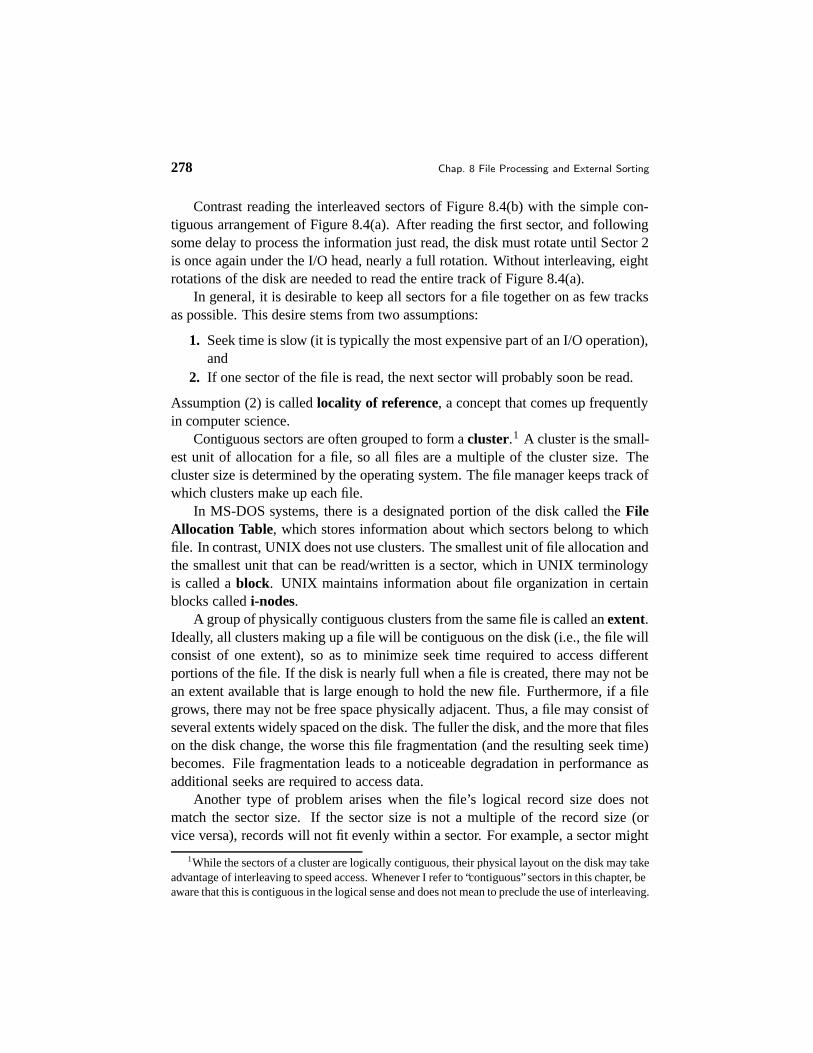


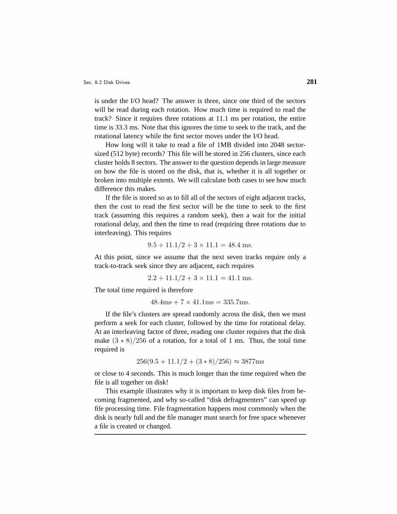


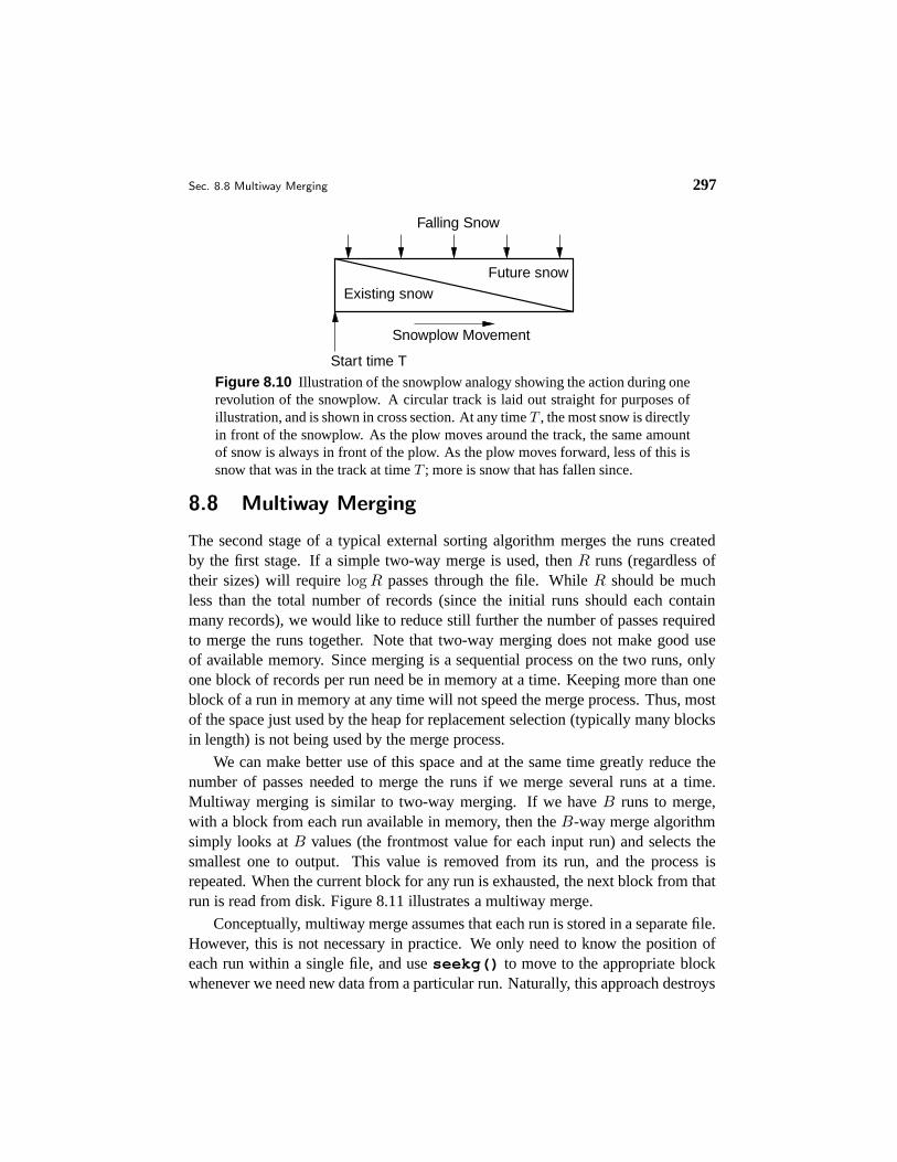

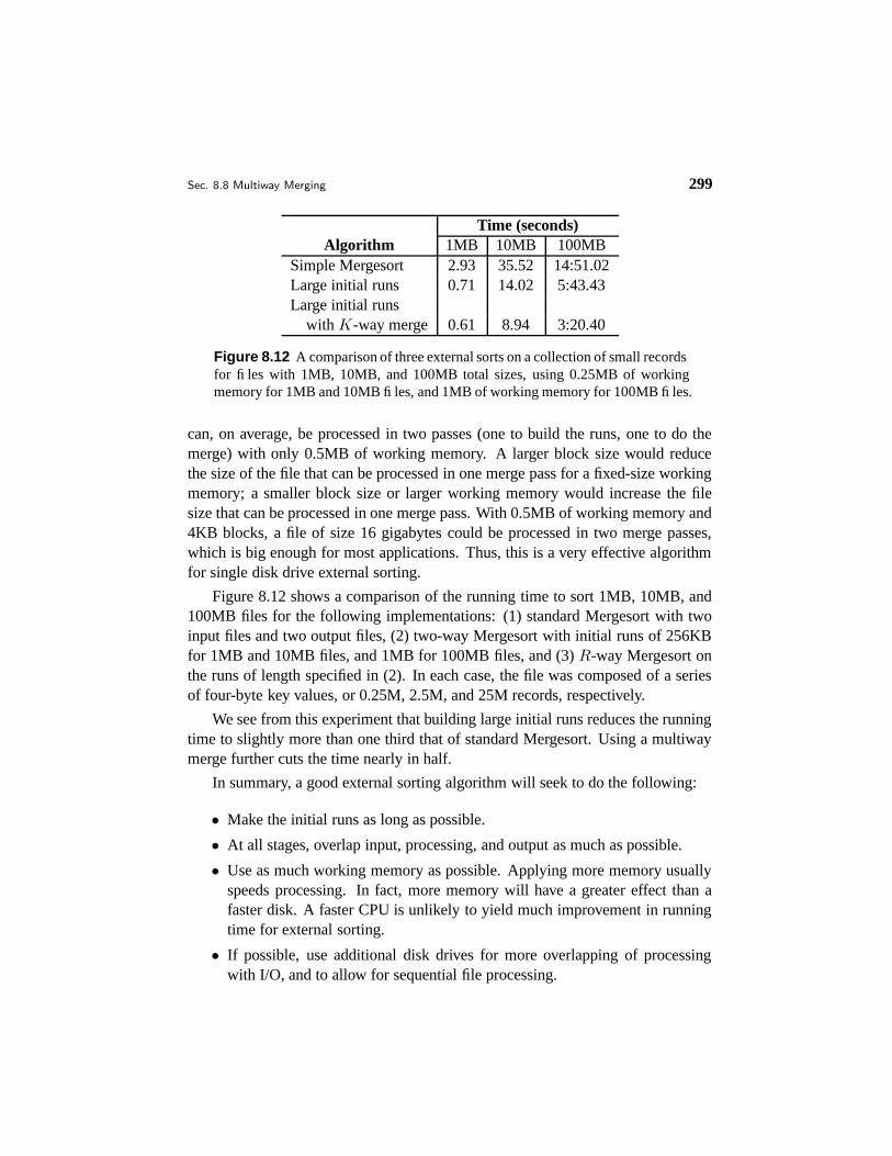


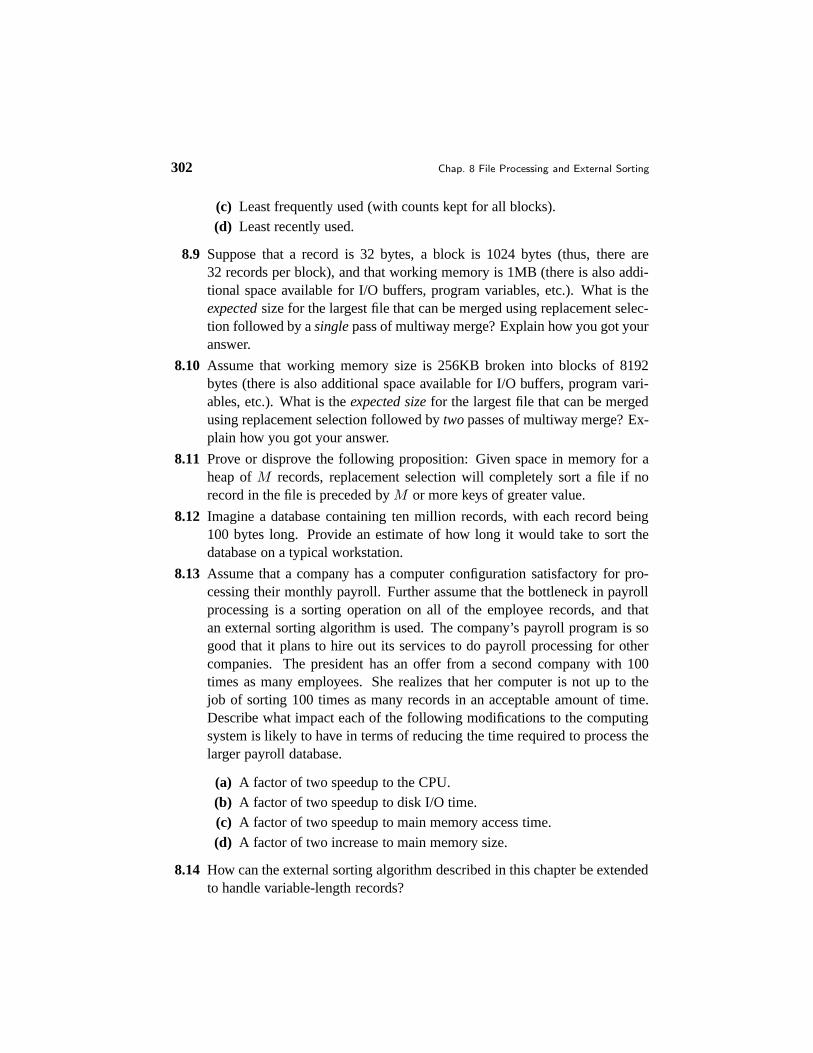
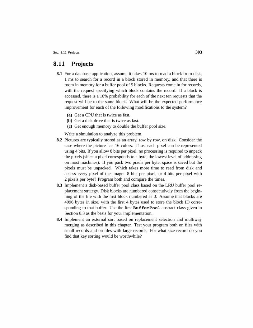


![C8 [File Processing & External Sorting]](https://static.documents.pub/doc/80x56/547f27bbb4af9fb9158b5944/c8-file-processing-external-sorting.jpg)
