158
8-lecture Mini-course in Quantum Computation Lecture 1 Lawrence Ioannou

8-lecture Mini-course in Quantum Computation
Lecture 1
Lawrence Ioannou

Topics Covered References^%*1 Basics I: motivation, interference, qubits, measurement Mosca: 1.1, 1.2
Textbook: 1.1.1 – 1.3.4
2 Basics II: gates, circuits Textbook: 4.1-4.4
3 Cool Applications: Bell states, superdense coding, no-cloning theorem, teleportation
Textbook: 1.3.5 - 1.3.7, 2.3
4 Algorithms I: models of computation, universality, relative phases, eigenvalue kick-back, Deutsch’s problem
Mosca: 2.1Textbook: 3.1, 4.5, 4.6, 4.7, 5.1, 5.2
5 Algorithms II: phase estimation, quantum Fourier transform (QFT), eigenvalue estimation, period-finding, order-finding
Mosca: 2.2, 2.3, 2.4, 2.5, 2.8.1, 2.9Textbook: 5.1, 5.2, 5.4.1, 5.3
6 Cryptographic applications: factoring N=pq, breaking the RSA cryptosystem, discrete logarithm problem (El Gamalcryptosystem), quantum key distribution
Mosca: A.5, 2.6Textbook: A4.3, 5.3, 5.4.2, 12.6.1, 12.6.3
7 Algorithms III: quantum searching, counting Mosca: 2.7Textbook: 6
8 Algorithms II*: review, Simon’s problem, hidden subgroup problem
quant-ph/9704027Mosca: 2.8Textbook: 5.4.3
% Mosca = Michele Mosca’s DPhil thesis, available at http://www.cacr.math.uwaterloo.ca/~mmosca/moscathesis.ps* quant-ph/xxxxxx = www.arxiv.org/quant-ph/xxxxxx^ Textbook = M. A. Nielsen and I. L. Chuang, “Quantum Computation and Information”, Cambridge University Press, 2000.

Motivation
Computation is a physical processe.g. neurons firing in your braine.g. electrons flowing through NAND gates in a
computer’s circuits
Therefore, laws of physics govern computation
“Classical physics” includesNewtonian mechanics (e.g. F=ma)Einstein’s General Relativityclassical electrodynamics (Maxwell’s equations)
c. 1905 experiments showed some of these laws to break down for small-scale systems (e.g. individual photons and electrons)

Motivation
“Quantum physics” replaced “classical physics” as the more correct theory describing the laws of nature
The Turing Machine (i.e. standard computer) can be implemented by physical phenomena that can be described by the laws of “classical physics”
Feynman (1982): But what if we build computers that use phenomena that can only be described by the laws of “quantum physics”?
Quantum computation was born...

Single-photon interferometer
Two paths through space, labelled “|0⟩” and “|1⟩”
|0⟩
|1⟩
Single-photon source, placed at start of |0⟩ path
ph|0⟩
(thick arrow represents trace of path taken by a photon)
|1⟩

Single-photon interferometer (2)
Add in some full-deflection mirrors (not shown), a beam-splitter* ( ), and some (photon) detectors ( )
ph|0⟩ 0(reflected photon)
(transmitted photon)
|1⟩ 1
A detector clicks when a photon hits it (no “half-clicks” occur)
Experiment: Have the photon-source emit one photon, and then record which detector clicks; repeat many times
Results: ~50% 0-clicks, ~50% 1-clicks
Reasonable conclusion: beam-splitter deflects photon with probability ½, and transmits photon with probability ½
*we will actually use Hadamard gates (introduced later), which are slightly different from beam-splitters; a beam-splitter can also be referred to as a “half-silvered mirror”

Single-photon interferometer (3)
Now add in some more full-deflection mirrors (not shown) and another beam-splitter
ph|0⟩
|1⟩
0
1
Repeat previous experiment
Surprising results: ~100% 0-clicks, ~0% 1-clicks
The previous conclusion is not complete, as we would have expected the same even distribution...

Single-photon interferometer (4)
Quantum-mechanical explanation of first experiment
ph|0⟩
The state of the photon can exist in a superposition of the two paths
When a photon in the |0⟩ path impinges on the beam-splitter, it exits in the state
⟩+⟩ 1|2
10|2
1
The probabilities of detecting the photon in the respective paths are obtained by squaring the moduli of the coefficients, which are complex numbers in general
0
|1⟩ 1

Single-photon interferometer (5)
Quantum-mechanical explanation of second experiment
ph|0⟩
When a photon in the |1⟩ path impinges on the beam-splitter, it exits in the state
⟩−⟩ 1|2
10|2
1
|1⟩
0
1
We say that the reflected beam picks up a phase of -1
The beam-splitter acts independently on each component in the superposition
Thus, the state of the photon after the second beam-splitter is
⟩=⎟⎠⎞
⎜⎝⎛ ⟩−⟩+⎟
⎠⎞
⎜⎝⎛ ⟩+⟩ 01
210
21
211
210
21
21
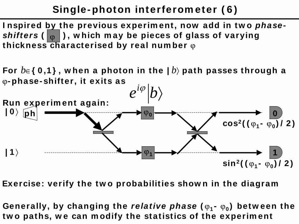
Single-photon interferometer (6)
Inspired by the previous experiment, now add in two phase-shifters ( ), which may be pieces of glass of varying thickness characterised by real number ϕ
ϕ
|0⟩
|1⟩
ph 0
1
ϕ0
ϕ1
cos2((ϕ1- ϕ0)/2)
sin2((ϕ1- ϕ0)/2)
Run experiment again:
For b∈{0,1}, when a photon in the |b⟩ path passes through a ϕ-phase-shifter, it exits as
⟩beiϕ
Exercise: verify the two probabilities shown in the diagram
Generally, by changing the relative phase (ϕ1- ϕ0) between the two paths, we can modify the statistics of the experiment

One Qubit
A (classical) bit is a two-level physical systemThe two levels are usually labelled “0” and “1”Let b be the state of the bit
“Classical physics” dictates that the bit may exist only in either the state 0 or 1:
b=0 or b=1
A quantum bit (qubit) is also a two-level physical systemThe two levels are usually labelled “|0⟩” and “|1⟩”Let |ψ⟩ be the (pure) state of the qubit
“Quantum physics” dictates that the qubit may exist in a complex superposition of |0⟩ and |1⟩:
|ψ⟩ = α|0⟩ + β|1⟩ (superposition principle)
where α and β are complex numbers such that |α|2+|β|2=1

One Qubit
A qubit is thus modelled by a two-dimensional complex vector space, C2, with (standard) orthonormal basis {|0⟩,|1⟩}, called the computational basis
The state |ψ⟩ of a qubit is modelled by a unit vector in this vector space
Physically, a qubit can be realised by
•the two degrees of freedom of two paths of a single photon (as we saw earlier)
•the two degrees of freedom of a spin-(1/2) particle: spin-up and spin-down)
•many other ways...

Don’t Freak Out: vector notation
In quantum mechanics, we use Dirac bra-ket notation to denote vectors
Standard notation Dirac notation
vr or v vvector
inner product vu rr• vu
dual vector v v†
or u†vstandard basis
{ }Neee ,...,, 21
{ }1,...,1,0 −N
⎥⎥⎥⎥⎥⎥⎥⎥⎥
⎦
⎤
⎢⎢⎢⎢⎢⎢⎢⎢⎢
⎣
⎡
=
0
010
0
M
M
jeor
{ }222 )1(,...,)1(,)0( −Nwhere (j)2 denotes the binary representation of j; i.e. labels are n-bit strings; when N=2n, each bit corresponds to a qubit
N = 2n
of CN
(ket)
(bra)
(elementary basis) (computational basis)
(represented as column-vector)
(represented as row-vector)

Measurement
The state of one qubit can encode an arbitrarily large amount of information
e.g. let α be such that its binary expansion encodes the Bibleα = 0.01001............11.........................000...110
“In the beginning...” “...Amen”
Then the state |ψ⟩ = α|0⟩ + β|1⟩ encodes many, many bits!
But we cannot access all the information directly!
The principle of quantum measurement dictates that measuring the qubit |ψ⟩ = α|0⟩ + β|1⟩ with respect to the computational basis yields
outcome 0 with probability |α|2, andoutcome 1 with probability |β|2
and, immediately after the measurement, the state of the qubit is the basis element labelled by the outcome
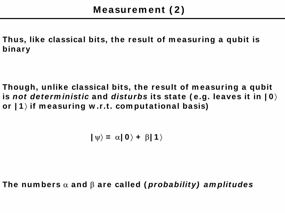
Measurement (2)
Thus, like classical bits, the result of measuring a qubit is binary
Though, unlike classical bits, the result of measuring a qubitis not deterministic and disturbs its state (e.g. leaves it in |0⟩or |1⟩ if measuring w.r.t. computational basis)
|ψ⟩ = α|0⟩ + β|1⟩
The numbers α and β are called (probability) amplitudes

Qubits
A two-qubit system is a system with 4 levels which correspond to the 4 combinations of the 2 levels in each qubit:
|0⟩|0⟩, |0⟩|1⟩, |1⟩|0⟩, |1⟩|1⟩
Again, the principle of quantum superposition says that the state |ϕ⟩ of the two-qubit system may be
|ϕ⟩ = α0|0⟩|0⟩ + α1|0⟩|1⟩ + α2|1⟩|0⟩ + α3|1⟩|1⟩
where |α0|2+|α1|2 +|α2|2 +|α3|2 =1 (αi are complex numbers)
Similar to before, measuring the two-qubit system with respect to the computational basis gives outcome
00 with probability |α0|2
01 with probability |α1|2
10 with probability |α2|2
11 with probability |α3|2

Qubits (2)
Mathematically, a two-qubit system is modelled by the tensor product (⊗) of two copies of the vector space that models a one-qubit system
E.g. let |ψ⟩A= α|0⟩A + β|1⟩A and |ψ⟩B = γ|0⟩B + δ|1⟩B be the states of two qubits; then the state |ψ⟩AB of the joint two-qubit system (in the order A,B) is
|ψ⟩AB = (α|0⟩A + β|1⟩A)⊗(γ|0⟩B + δ|1⟩B)= αγ|0⟩A⊗|0⟩B + αδ|0⟩A⊗|1⟩B + βγ|1⟩A⊗|0⟩B + βδ|1⟩A⊗|1⟩B
which is usually just written
αγ|00⟩ + αδ|01⟩ + βγ|10⟩ + βδ|11⟩
and the order of systems A and B remembered
Note that the tensor product makes sense in light of the measurement principle and probability theory: e.g. the probability of getting outcome |01⟩ is the probability of getting |0⟩ for qubit A and |1⟩ for qubit B (assuming independence of events)

Qubits (3)
In general, an n-qubit system (register) is modelled by the tensor product (⊗) of n copies of C2
The state |ψ⟩ of an n-qubit register is a complex unit vector in this tensor product space, often written in the computational basis as
|ψ⟩ = ∑−
=
⟩12
0|
n
ii iα
where the index is viewed in its n-bit binary representation when inside the “| ⟩”, and
∑−
=
=12
0
2 1||n
iiα
Measuring the n-qubit register with respect to the computational basis gives outcome
with probability ⟩i| 2|| iα

More Measurement
More generally, one can measure with respect to (orthonormal) basis B={|bi⟩}
If B is a basis for the vector space containing |ψ⟩ , then the state (expressed in the computational basis)
|ψ⟩ = ∑−
=
⟩12
0|
n
ii iα
|ψ⟩ = ∑−
=
⟩12
0|
n
iii bβ
may also be written
Measurement of the qubit system with respect to basis B gives outcome
with probability ib 2|| iβ
and, immediately after the measurement, the state of the qubit system is the basis element labelled by the outcome

More Measurement (2)
E.g. for two-qubit systems, an interesting basis other than the computational (standard) basis is the Bell basis, consisting of the four Bell states:
|00⟩ + |11⟩|00⟩ - |11⟩|01⟩ + |10⟩|01⟩ - |10⟩
where we have omitted the normalisation factor of in each state. 2
1
We’ll return to these states later... they are very important for communication protocols and quantum cryptography!

8-lecture Mini-course in Quantum Computation
Lecture 2
Lawrence Ioannou

Quantum Gates
Recall the classical gates (for bits b, c, d):
1-b (one-bit) NOT gateb
c(two-bit) NAND gate1 – cd
d
What should a quantum gate be like?
?|ψ⟩ |ψ’⟩
Since |ψ⟩ and |ψ’⟩ are quantum states, the gate should preserve vector norm. Notice that a unitary operator has this property....
(Recall: U is unitary means U-1=U†, where † denotes complex-conjugate transpose operation, i.e. complex conjugate of each matrix element followed by matrix transpose operation)

Quantum Gates
In general, quantum gates are unitary operators
U|ψ⟩ |ψ’⟩
Note that the number of input qubits always equals the number of output qubits
Since all unitary operators have an inverse, all quantum gates are reversible
|ψ⟩|ψ⟩ U U†
which means no heat need be dissipated during a computation (Landauer’s principle)
(Classical computing can also be made reversible)

Matrix Representations
When doing calculations, often it is useful to represent the state of a qubit-register and the operations (gates) applied to it by matrices with respect to the computional basis
Technically, we can use the notation “[...]” to distinguish the state or operator from its matrix representation:
⎥⎦
⎤⎢⎣
⎡βα
e.g. |ψ⟩ = α|0⟩ + β|1⟩ is represented as [|ψ⟩] =
e.g. the one-qubit gate U which maps
|0⟩ → a|0⟩ +b|1⟩|1⟩ → c|0⟩ +d|1⟩
is represented as [U]=⎥⎦
⎤⎢⎣
⎡dbca
When the basis is understood to be the computational basis, we may drop the “[...]” notation (especially for states)
e.g. we may write U|ψ⟩ = [U][|ψ⟩]

Some Important One-qubit Gates
U|ψ⟩ = [U]U⎥⎦
⎤⎢⎣
⎡βα
⎢⎣
⎡βα⎥⎦
⎤|ψ⟩=
(input) (output)
Hadamard ⎥⎦
⎤⎢⎣
⎡−1111
21
Pauli-X (NOT) ⎥⎦
⎤⎢⎣
⎡0110
Pauli-Y ⎥⎦
⎤⎢⎣
⎡ −0
0i
i
Pauli-Z ⎥⎦
⎤⎢⎣
⎡−1001
θ-phase ⎥⎦
⎤⎢⎣
⎡θie0
01
U [U] Gate symbol
H
Rθ
X
Y
Z

Two-Qubit Gates
U|ψ⟩= U|ψ⟩ = [U]
⎥⎥⎥⎥
⎦
⎤
⎢⎢⎢⎢
⎣
⎡
3
2
1
0
αααα
⎥⎥⎥⎥
⎦
⎤
⎢⎢⎢⎢
⎣
⎡
3
2
1
0
αααα
Two one-qubit gates acting in parallel constitute a two-qubitgate:
U1
U0
If U is the operator corresponding to this 2-qubit gate, how is U represented mathematically in terms of U0 and U1?
ANSWER: tensor product!U = U0⊗U1
Matrix tensor product: the tensor product M⊗N of two matrices M and N is the block matrix:
[MijN]
where Mij is the element of M in the ith row and jth column

Controlled-Operations (two-qubit gates)
But, in general, a two-qubit gate is not the tensor product of two one-qubit gates!
Suppose U is a one-qubit operation U
We can define the operation on qubits A and B that maps
|0⟩A|ψ⟩B → |0⟩A|ψ⟩B|1⟩A|ψ⟩B → |1⟩AU|ψ⟩B
Classically: “If qubit A is in state |1⟩, then apply U to qubit B; otherwise do nothing”
This is the controlled-U gate, with control qubit A and target qubit B.
For general U, controlled-U cannot be written as a tensor product of two one-qubit gates
A
B U
Gate symbol:

Two Important Two-qubit Gates
U U|ψ⟩ = [U]⎥⎥⎥⎥
⎦
⎤
⎢⎢⎢⎢
⎣
⎡
3
2
1
0
αααα
⎥⎥⎥⎥
⎦
⎤
⎢⎢⎢⎢
⎣
⎡
3
2
1
0
αααα
|ψ⟩=
All matrices are with respect to the computational basis with the following qubit ordering
{|0⟩A|0⟩B , |0⟩A|1⟩B , |1⟩A|0⟩B , |1⟩A|1⟩B }
⎥⎥⎥⎥
⎦
⎤
⎢⎢⎢⎢
⎣
⎡
0100100000100001
Controlled-NOT (CNOTA,B)
U [U] Gate symbol
qubit A (control)
qubit B (target)
⎥⎥⎥⎥
⎦
⎤
⎢⎢⎢⎢
⎣
⎡
1000001001000001SWAPA,B
x
x
(maps |ψ⟩A|ϕ⟩B → |ϕ⟩A|ψ⟩B)

Quantum Networks
A quantum network (diagram) is a tool we use to describe a (complex) quantum operation usually as a sequence of (simpler) operations
It is a concatenation of gate symbols, read from left to right
Each horizontal line represents one qubit
To represent a particular computation, the initial (input) state(of each qubit) may be written on the left of the diagram; the final (output) state may be written on the right.
E.g. (a three-qubit quantum network)
|0⟩|ψ’⟩X|0⟩
|0⟩

Computing U and |ψ’⟩
X
|0⟩|0⟩|0⟩
|ψ’⟩
U=U3U2U1
U1 U2 U3
Label the qubits from top to bottom: A, B, C
Fix a computational basis with the corresponding ordering:{|0⟩A|0⟩B |0⟩c , |0⟩A|0⟩B |1⟩c ,..., |1⟩A|1⟩B |1⟩c}
Reading from left to right, U is made up of three operations U1 (CNOTA,B), U2 (CNOTC,A), and U3 (NOTB):
|ψ’⟩ = U3U2U1|000⟩
Let’s calculate the matrix representations of each operation...

Computing U and |ψ’⟩
Computing [U1] (CNOTA,B)
Let I be the identity operator (no action on qubit(s))U1 = CNOTA,B ⊗ I
[U1] =
⎥⎥⎥⎥⎥⎥⎥⎥⎥⎥⎥
⎦
⎤
⎢⎢⎢⎢⎢⎢⎢⎢⎢⎢⎢
⎣
⎡
=⎥⎦
⎤⎢⎣
⎡⊗
⎥⎥⎥⎥
⎦
⎤
⎢⎢⎢⎢
⎣
⎡
1001
1001
1001
1001
1001
0100100000100001
(zeros elsewhere)

Computing U and |ψ’⟩
Computing [U2] (CNOTC,A)
Either directly from mapping of computational basis:
|x⟩A|x⟩B|0⟩C → |x⟩A|x⟩B|0⟩C|x⟩A|x⟩B|1⟩C → |1-x⟩A|x⟩B|1⟩C x∈{0,1}
or, notice that
CNOTC,A=(SWAPB,C)(CNOTB,A)(SWAPB,C)
[U2] =
⎟⎟⎟⎟⎟
⎠
⎞
⎜⎜⎜⎜⎜
⎝
⎛
⎥⎥⎥⎥
⎦
⎤
⎢⎢⎢⎢
⎣
⎡
⊗⎥⎦
⎤⎢⎣
⎡
⎟⎟⎟⎟⎟
⎠
⎞
⎜⎜⎜⎜⎜
⎝
⎛
⎥⎦
⎤⎢⎣
⎡⊗
⎥⎥⎥⎥
⎦
⎤
⎢⎢⎢⎢
⎣
⎡
⎟⎟⎟⎟⎟
⎠
⎞
⎜⎜⎜⎜⎜
⎝
⎛
⎥⎥⎥⎥
⎦
⎤
⎢⎢⎢⎢
⎣
⎡
⊗⎥⎦
⎤⎢⎣
⎡
10110
1
1001
1001
11
11
10110
1
1001
(zeros elsewhere)

Computing U and |ψ’⟩
Computing [U3] (NOTB)
U3 = I⊗X⊗I
⎥⎦
⎤⎢⎣
⎡⊗⎥
⎦
⎤⎢⎣
⎡⊗⎥
⎦
⎤⎢⎣
⎡1001
0110
1001[U3] =
Thus, [U]=[U3][U2][U1]
[|ψ’⟩] =[U][|000⟩] To compute [|ψ’⟩] :
= [U3][U2][U1]
⎥⎥⎥⎥⎥⎥⎥⎥⎥⎥⎥
⎦
⎤
⎢⎢⎢⎢⎢⎢⎢⎢⎢⎢⎢
⎣
⎡
00000001

Single-photon interferometer as a quantum network diagram
The interferometry experiment
ph|0⟩ ϕ0
|1⟩ ϕ1
is represented by
H Rθ H|0⟩
θ = ϕ1 - ϕ0

Properties of Tensor Product ⊗
A⊗B ≠ B⊗A
A⊗B⊗C = (A⊗B)⊗C = A⊗(B⊗C)
A⊗(B+C) = A⊗B + A⊗C
(A+B)⊗C = A⊗C +B⊗C
for scalar α: α(A⊗B) = (αA)⊗B = A⊗(αB)
for operators U,V: (U⊗V)(|ψ⟩⊗|ϕ⟩) = (U|ψ⟩)⊗(V|ϕ⟩)
for matrices M,N: M⊗N = [MijN] (in block form)where Mij is the element of M in the ith row and jth column
we normally omit the symbol ⊗ when it is between states

8-lecture Mini-course in Quantum Computation
Lecture 3
Lawrence Ioannou

Entangled States
Let |ψ⟩A= α|0⟩A + β|1⟩A and |ψ⟩B = γ|0⟩B + δ|1⟩B be the states of two qubits; then the state |ψ⟩AB of the joint two-qubit system is
|ψ⟩AB = (α|0⟩A + β|1⟩A) ⊗ (γ|0⟩B + δ|1⟩B)
The state |ψ⟩AB is a special kind of two-qubit state called a separable state, because it is the tensor-product of the states of the two constituent qubits
A two-qubit state which is not separable is called an entangled state
e.g. |00⟩ + |11⟩ (omitting normalisation factors)
Exercise: Prove that |00⟩ + |11⟩ is entangled, i.e. show that there do not exist α, β, γ, δ such that |00⟩ + |11⟩ equals
(α|0⟩ + β|1⟩) ⊗ (γ|0⟩ + δ|1⟩)

Entangled States (2)
e- e-(counter-intuitive correlations)
(possibly large distance)
We say that two qubits are entangled when their state is an entangled state
Intuitively, entangled qubits can be thought to be “linked” in some elusive, unintuitive way
Even if the two entangled qubits (e.g. two electrons) are physically separated (taken kilometers away from each other), they still remain “linked”
This elusive nonclassical (quantum) correlation between the two physically separated entangled qubits can be exploited to transfer information!

Bell States (EPR pairs)
|β00⟩ =|00⟩ + |11⟩|β01⟩ =|01⟩ + |10⟩
Four special entangled two-qubit states are the Bell states or EPR pairs:
|β10⟩ =|00⟩ - |11⟩|β11⟩ =|01⟩ - |10⟩
Note that the following quantum network maps |bc⟩ to |βbc⟩
H|b⟩|βbc⟩
|c⟩
Exercise: show how a similar network can be used to effect a measurement w.r.t. the Bell basis by actually measuring w.r.t. the computational basis

Superdense Coding
Superdense coding is a two-party protocol that utilises a shared EPR pair in order to communicate two classical bits from one party (Alice) to the other (Bob) while only communicating one of the shared qubits
Suppose Alice and Bob each have one qubit of the state|β00⟩ =|00⟩ + |11⟩
(Alice’s qubit is on the left, Bob’s on the right...)
Alice wishes to send two classical bits b,c to Bob
I⊗I |β00⟩ = |β00⟩Y⊗I |β00⟩ = |β01⟩
By operating only on her qubit, Alice can transform |β00⟩ into any of the four Bell states:
X⊗I |β00⟩ = |β10⟩Z⊗I |β00⟩ = |β11⟩
Protocol: Alice transforms |β00⟩ into |βbc⟩, and then sends her qubit to Bob. Bob measures the two qubits w.r.t. the Bell basis.

No-cloning Theorem
Suppose Alice would like to send a copy of her arbitrary qubitto Bob
She cannot!
Suppose that some quantum operation O maps
|ψ⟩ → |ψ⟩|ψ⟩for all states |ψ⟩
Then O must map |ψ⟩ → |ψ⟩|ψ⟩|ϕ⟩ → |ϕ⟩|ϕ⟩
|ψ⟩+|ϕ⟩ → (|ψ⟩ + |ϕ⟩)(|ψ⟩ + |ϕ⟩)
But O is a quantum operation, so it must be linear and thus map |ψ⟩+|ϕ⟩ → |ψ⟩|ψ⟩ + |ϕ⟩|ϕ⟩
This is a contradiction, thus O cannot exist

Quantum Teleportation(Quantum) Teleportation is a two-party protocol that utilisesa shared EPR pair in order to send one qubit from Alice to Bob while only communicating two classical bits
This does not violate the no-cloning theorem because Alice destroys the state of her qubit in the process
As in superdense coding, Alice and Bob share EPR pair |β00⟩(with Alice’s qubit on the left)
Suppose Alice wants to send the qubit |ψ⟩ to Bob
Exercise: verify |ψ⟩ ⊗|β00⟩ = |β00⟩ ⊗|ψ⟩+ |β01⟩ ⊗X|ψ⟩+ |β10⟩ ⊗Z|ψ⟩+ |β11⟩ ⊗XZ|ψ⟩
Protocol: Alice measures her two qubits w.r.t. the Bell basis getting outcome βbc, and then sends bits b,c to Bob. Bob applies ZbXc to his qubit (note X2=Z2=I).

Quantum Network Diagram for Teleportation
H b
c
Bell Measurement
Xc Zb
double lines represent flow of classical information
|ψ⟩
|ψ⟩|β00⟩
This symbol represents measurement of a qubit with respect to the computational basis; the output of this “measurement gate” is classical (0 or 1)
Xc This symbol means “if c=0, do nothing, else apply X gate”; it is a classically-controlled quantum gate
In the teleportation protocol, the upper two qubits belong to Alice and the bottom qubit belongs to Bob
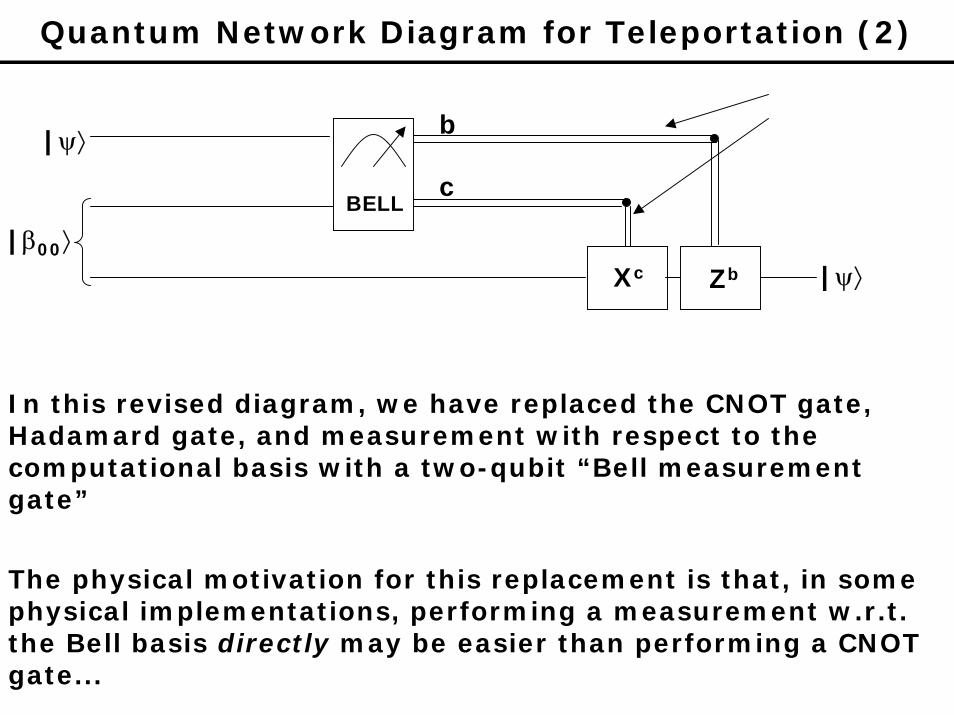
Quantum Network Diagram for Teleportation (2)
b
c
Xc Zb
|ψ⟩
|ψ⟩|β00⟩
BELL
In this revised diagram, we have replaced the CNOT gate, Hadamard gate, and measurement with respect to the computational basis with a two-qubit “Bell measurement gate”
The physical motivation for this replacement is that, in some physical implementations, performing a measurement w.r.t. the Bell basis directly may be easier than performing a CNOT gate...

Teleportation: Not just a pretty face
...based on this assumption, teleportation can be used to fight against errors in the implementation of quantum gates.
It may be that a particular implementation of the CNOT gate is not perfect (fails with some probability)
If a CNOT gate fails midway through a complex computation, then the entire computation might be ruined
Normally, quantum error-correction codes are used to fight against errors
Alternatively, teleportation can be used to reduce the application of an imperfect CNOT gate to the preparation of a particular 4-qubit entangled state
|Ψ⟩ = (|0000⟩ + |0011⟩ + |1110⟩ + |1101⟩)/2
Instead of a CNOT gate possibly failing, the preparation of |Ψ⟩may fail (but this failure does not ruin the computation)

Teleportation: Not just a pretty face (2)
The following sequence of equivalent network diagrams illustrates the method
α|0⟩ + β|1⟩
γ|0⟩ + δ|1⟩
Diagram 1

Teleportation: Not just a pretty face (3)
α|0⟩ + β|1⟩
γ|0⟩ + δ|1⟩
H
H
H
H
c
Xc Zb
b
Xe Zd
|0⟩
|0⟩
|0⟩
|0⟩
d
e
Diagram 2
Added four ancillary qubits in order to teleport the outer two qubits to the inner two qubits, and then apply the CNOT to the inner two qubits

Teleportation: Not just a pretty face (4)
α|0⟩ + β|1⟩
γ|0⟩ + δ|1⟩
H
H
H
H
c
Xc Zb
b
Xe Zd
d
e
|0⟩
|0⟩
|0⟩
|0⟩
Diagram 3
Added two CNOT gates on the inner two qubits

Teleportation: Not just a pretty face (5)
α|0⟩ + β|1⟩
H
H
c
Xc Zb
b
Xe Zd
d
eγ|0⟩ + δ|1⟩
|0⟩
|0⟩
|0⟩
|0⟩
BELL
BELL
Diagram 4
Replaced two instances of CNOT, Hadamard, and measurement w.r.t. computational basis with “Bell measurement gate” (based on assumption that a direct Bell measurement may be easier to implement than a CNOT gate)
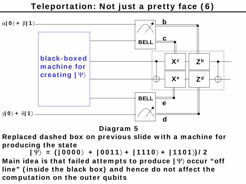
Teleportation: Not just a pretty face (6)
c
Xc Zb
b
Xe Zd
d
e
α|0⟩ + β|1⟩
γ|0⟩ + δ|1⟩
Diagram 5Replaced dashed box on previous slide with a machine for producing the state
BELL
BELL
|Ψ⟩ = (|0000⟩ + |0011⟩ + |1110⟩ + |1101⟩)/2
black-boxed machine for creating |Ψ⟩
Main idea is that failed attempts to produce |Ψ⟩ occur “off line” (inside the black box) and hence do not affect the computation on the outer qubits

Teleportation: Not just a pretty face (7)
α|0⟩ + β|1⟩
BELL
BELL
black-boxed machine for creating |Ψ⟩
classical logic
Z
X
X
Z
γ|0⟩ + δ|1⟩
Diagram 6
Exercise: Show that this final replacement is valid; i.e. show that the two CNOT gates in the dashed box on the previous slide can be removed as long as the classical logic controlling the X and Z gates is appropriately modified

8-lecture Mini-course in Quantum Computation
Lecture 4
Lawrence Ioannou

Models of Computation
Recall the polytime-equivalent classical models:
Turing Machine•Idealised computer•Two-way infinite tape, mobile read/write head, CPU (transfer function)
00 0 0 0 1 1 1
CPU
1 1
Reversible acyclic gate array (reversible circuit model)
input output

Model of Computation (2)
Although one can define a quantum Turing Machine, we will use the quantum analogue of the classical reversible circuit model, known as the quantum circuit model
More specifically, we restrict to uniform families of quantum networks (or quantum gate arrays, or quantum circuits):
For a given problem, there exists a classical Turing Machine that, given the input size, n, of an instance of the problem, generates a quantum network diagram to solve the instance in poly(n) steps
This ensures that the proposed quantum solution of the problem is (considered) efficient
Such a uniform family of quantum networks is an efficient algorithm

Universality
Recall that the gates AND, OR, and NOT (or just the NAND-gate) are universal for classical (non-reversible) computation
For reversible classical computation, the three-bit Toffoli gate(or controlled-controlled-NOT) is universal
aabbc⊕(ab)c
Toffoli gate
Universality (2)
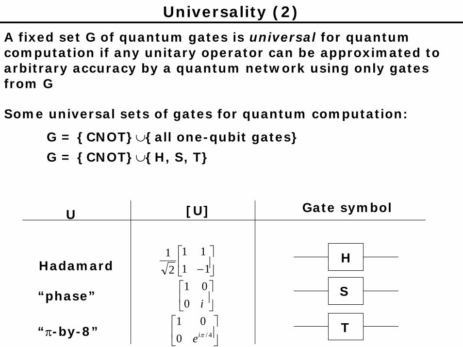
A fixed set G of quantum gates is universal for quantum computation if any unitary operator can be approximated to arbitrary accuracy by a quantum network using only gates from G
Some universal sets of gates for quantum computation:
G = {CNOT}∪{all one-qubit gates}
G = {CNOT}∪{H, S, T}
Hadamard ⎥⎦
⎤⎢⎣
⎡−1111
21
⎥⎦
⎤⎢⎣
⎡4/0
01πie
⎥⎦
⎤⎢⎣
⎡i001
U [U]
“phase”
“π-by-8”
Gate symbol
H
S
T

What’s so great about quantum algorithms
Efficient quantum algorithms exist for problems such as INTEGER FACTORING and DISCRETE LOGARITHM
•INTEGER FACTORING: Given integer N, such that N=pq for odd prime numbers p and q; find p
•DISCRETE LOGARITHM: Given integers N, b, y; find integer x such that y = bx mod N (i.e. N divides bx with remainder y)
•Efficient classical algorithms are not known to exist for these problems which form the basis for computational secure cryptosystems like RSA and El Gamal
Quantum algorithms can efficiently simulate quantum physics (see 4.7 in textbook)

Problems as black box functions
Many computational problems can be expressed in terms of a black box function f
f: G → {0,1,...,N-1}
where the “answer” to the problem is some (hidden) property of f (G is some set)
We assume that we can query the black box, i.e. give it an input x and get out f(x) (reversibly)
⊕f(x)
|x⟩
|y⊕f(x)⟩
|x⟩
|y⟩
here, “⊕” means bit-wise addition modulo 2

Problems as black box functions (2)
Some examples:
Searching problem:
Given black box for f: {0,1}n → {0,1}
Find an x such that f(x)=1
({0,1}n is the “database”)
Period-finding problem:
Given black box for f: {0,1,…} → {0,1,…,N-1}, where f is periodic, f(x+r)=f(x)
Find the period r
e.g. f(x)=ax mod N (related to INTEGER FACTORING)

Classical v. Quantum ComputersThe state of a classical reversible computer is confined to being one of the computational basis states at any time (queries to the black box for f can only be made one at a time)
Quantum computers can branch out over exponentially many computational basis states, like
∑−
=
⟩12
0
|21n
nx
x
Using the black box for f only once, one can then evaluate f(x) for exponentially many x in superposition:
∑−
=
⟩⟩12
0)(||
21n
nx
xfx
Such states can be further processed (quantumly) to extract hidden properties of f

Randomised Classical v. Quantum Computers (1)
Recall that a deterministic computation can be regarded as a path through “configuration space” of all configurations of a Turing machine (each configuration corresponds to an element of the computational basis)
A randomised computation can be regarded as a tree
|001⟩
|010⟩
|000⟩
|011⟩
|101⟩
|111⟩
|110⟩p0
p1
p2
p3
p4
p5
p6
p7
p8
p9
|000⟩
where each branch has a probability pi associated with it

|000⟩
|001⟩
|010⟩
|000⟩
|011⟩
|101⟩
|111⟩
|110⟩p0
p1
p2
p3
p4
p5
p6
p7
p8
p9
Randomised Classical v. Quantum Computers (2)
The outcome |000⟩ in this computation can be reached by two paths (red and green)
Probability of reaching |000⟩ by the red path is |a00|2 =p0p3
Probability of reaching |000⟩ by the green path is |a10|2 =p2p4
The total probability of reaching |000⟩ is thus |a00|2 + |a10|2

Randomised Classical v. Quantum Computers (3)
In our interferometry experiment, recall that there are two “computational paths” that lead to the outcome 0 (red path and green path):
ph|0⟩ 0
1
ϕ0
ϕ1
cos2((ϕ1- ϕ0)/2)
|1⟩
The probability amplitude of reaching 0 by the red path is a00 = exp(iϕ0)/2
The probability amplitude of reaching 0 by the green path is a10 = exp(iϕ1)/2
The total probability of reaching 0 is
|a00 + a10|2= cos2((ϕ1- ϕ0)/2)

Randomised Classical v. Quantum Computers (4)
|0⟩
|1⟩
ph 0
1
ϕ0
ϕ1
a00 = exp(iϕ0)/2
a10 = exp(iϕ1)/2
The total probability of reaching 0 is |a00 + a10|2= cos2((ϕ1- ϕ0)/2)
The relative phase between the probability amplitudes of the two paths matters (no such concept in the classical case), and can result in constructive or destructive interference
e.g. destructive interference occurs when a00 = -a10,
e.g. constructive interference occurs when a00 = a10
One goal of quantum algorithms is to induce constructive interference on good outcomes and destructive interference on bad outcomes

Quantum Algorithms as Interferometry
Most quantum algorithms can be viewed as big interferometry experiments
ph|0⟩ 0
1
ϕ0
ϕ1
cos2((ϕ1- ϕ0)/2)
sin2((ϕ1- ϕ0)/2)|1⟩
≡
H Rϕ H|0⟩
ϕ = ϕ1 - ϕ0
Basic idea: the measurement can distinguish the two cases ϕ=0 and ϕ=π
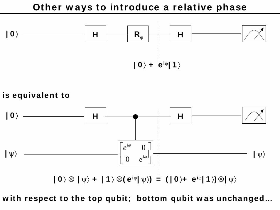
Other ways to introduce a relative phase
H Rϕ H
|0⟩ + eiϕ|1⟩
|0⟩
is equivalent to
H H
⎥⎦
⎤⎢⎣
⎡ϕ
ϕ
i
i
ee0
0
|0⟩ ⊗ |ψ⟩ + |1⟩ ⊗(eiϕ|ψ⟩) = (|0⟩+ eiϕ|1⟩)⊗|ψ⟩
|0⟩
|ψ⟩ |ψ⟩
with respect to the top qubit; bottom qubit was unchanged…

Other ways to introduce a relative phase (2)
… more generally, the bottom qubit will “kick back” a relative phase (eigenvalue) in the top qubit if the bottom qubit is in an eigenstate of U:
H H|0⟩
|ψ⟩ |ψ⟩U
(|0⟩+ eiϕ|1⟩)⊗|ψ⟩
where
U|ψ⟩ = eiϕ|ψ⟩
This so-called “eigenvalue kick-back” is a useful mechanism by which to analyse (though, not necessarily implement) quantum algorithms
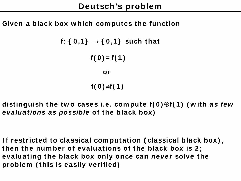
Deutsch’s problem
Given a black box which computes the function
f: {0,1} → {0,1} such that
f(0)=f(1)
or
f(0)≠f(1)
distinguish the two cases i.e. compute f(0)⊕f(1) (with as few evaluations as possible of the black box)
If restricted to classical computation (classical black box), then the number of evaluations of the black box is 2; evaluating the black box only once can never solve the problem (this is easily verified)

Deutsch’s problem (2)
However, suppose one has a quantum gate that computes f:
⊕f(x)
|x⟩
|y⊕f(x)⟩
|x⟩
|y⟩
for x,y∈{0,1}
Then the following quantum network solves Deutsch’s problem with probability ½
⊕f(x)
H H|0⟩
|0⟩

Deutsch’s problem (3)
⊕f(x)
H H|0⟩
|ψ1⟩ |ψ2⟩
|0⟩
|ψ1⟩ = |0⟩|f(0)⟩ + |1⟩|f(1)⟩
|ψ2⟩ = (|0⟩+|1⟩)|f(0)⟩ + (|0⟩-|1⟩)|f(1)⟩
= |0⟩(|f(0)⟩+|f(1)⟩) + |1⟩(|f(0)⟩-|f(1)⟩)
If f(0)=f(1), then cannot measure outcome 1 in upper qubit
Thus, if one does get outcome 1, then one may conclude that f(0)≠f(1) (if one gets outcome 0, then either case may hold)
This solution to Deutsch’s problem is already better (on average) than any classical solution; but we can do better…

Deutsch’s problem (4)
⊕f(x)
H H|0⟩
|ψ1⟩ |ψ2⟩
|0⟩
Note |ψ1⟩ = |0⟩|f(0)⟩ + |1⟩|f(1)⟩
= [|0⟩+|1⟩] (|0⟩+|1⟩) + [(-1)f(0)|0⟩ + (-1)f(1)|1⟩](|0⟩-|1⟩)
= [|0⟩+|1⟩] (|0⟩+|1⟩) + (-1)f(0) [|0⟩ + (-1)f(0)+f(1)|1⟩](|0⟩-|1⟩)
Now |ψ2⟩ = |0⟩(|0⟩+|1⟩) + (-1)f(0)|f(0)⊕f(1)⟩(|0⟩-|1⟩)
The measurement now clearly gives the answer f(0)⊕f(1) with probability 50% (the other half of the time, the measurement gives 0, which is inconclusive)

Deutsch’s problem (5)
⊕f(x)
H H|0⟩
|ψ1⟩ |ψ2⟩
|0⟩
|ψ1⟩ = |0⟩|f(0)⟩ + |1⟩|f(1)⟩
= [|0⟩+|1⟩] (|0⟩+|1⟩) + [(-1)f(0)|0⟩ + (-1)f(1)|1⟩](|0⟩-|1⟩)
|ψ2⟩ = |0⟩(|0⟩+|1⟩) + (-1)f(0)|f(0)⊕f(1)⟩(|0⟩-|1⟩)
BIG IDEA: |x⟩(|0⟩+|1⟩) and |x⟩(|0⟩-|1⟩) are eigenvectors of the operation |x⟩|b⟩ → |x⟩|b⊕f(x)⟩, with eigenvalues 1 and (-1)f(x)
Thus the controlled-(⊕f(x)) gate actually induces a relative phase in the top qubit, via an eigenvalue kick-back
Since the |0⟩-|1⟩ eigenvector is the one that produces the desired relative phase in the top qubit…

Deutsch’s problem (6)
⊕f(x)
H H|0⟩
|ψ1⟩ |ψ2⟩
|0⟩-|1⟩ |0⟩-|1⟩
|ψ1⟩ = [(-1)f(0)|0⟩ + (-1)f(1)|1⟩](|0⟩-|1⟩)
|ψ2⟩ = (-1)f(0)|f(0)⊕f(1)⟩(|0⟩-|1⟩)
This revised algorithm succeeds with probability 1
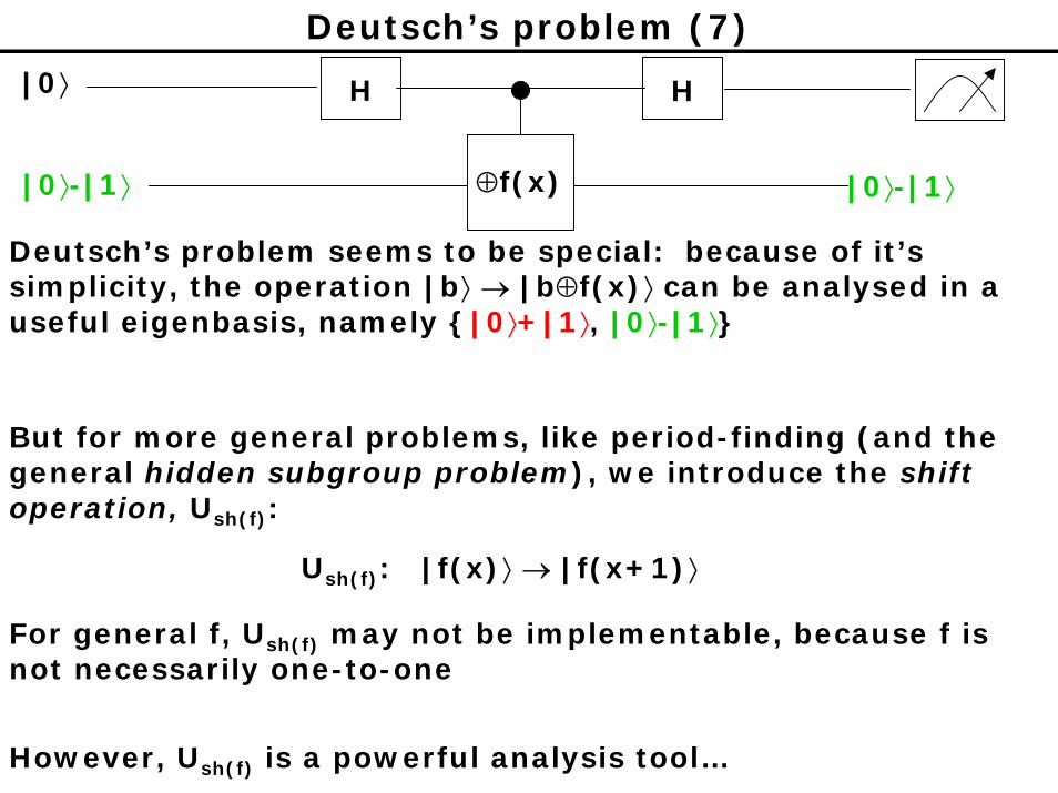
Deutsch’s problem (7)
H H|0⟩
⊕f(x)|0⟩-|1⟩ |0⟩-|1⟩
Deutsch’s problem seems to be special: because of it’s simplicity, the operation |b⟩ → |b⊕f(x)⟩ can be analysed in a useful eigenbasis, namely {|0⟩+|1⟩, |0⟩-|1⟩}
But for more general problems, like period-finding (and the general hidden subgroup problem), we introduce the shift operation, Ush(f):
Ush(f): |f(x)⟩ → |f(x+1)⟩
For general f, Ush(f) may not be implementable, because f is not necessarily one-to-one
However, Ush(f) is a powerful analysis tool…

Deutsch’s problem (8)
⊕f(x)
H H|0⟩
|0⟩-|1⟩ |0⟩-|1⟩
Instead of the controlled-⊕f(x) gate (above), assume we have a controlled-Ush(f) gate which maps
|0⟩|f(x)⟩ → |0⟩|f(x)⟩|1⟩|f(x)⟩ → |0⟩|f(x+1)⟩
Ush(f)
H H|0⟩

Deutsch’s problem (9)
Ush(f)
H H|0⟩
Note: f(0)=f(1) implies Ush(f) = If(0)≠f(1) implies Ush(f) = X
Both I and X have eigenvectors {|0⟩+|1⟩,|0⟩-|1⟩}, but I has eigenvalues {1,1} whereas X has eigenvalues {1,-1}
So, Ush(f) has eigenvectors {|0⟩+|1⟩,|0⟩-|1⟩} with eigenvalues
{1, (-1)f(0)⊕f(1)}
or, writing the eigenvalues another way,
{1, eiπf(0)⊕f(1)}

Deutsch’s problem (10)
Ush(f)
H H|0⟩
Eigenvalues of Ush(f) are {1, eiπf(0)⊕f(1)}
Thus, the answer f(0)⊕f(1) is encoded in the “phase” of an eigenvalue of the shift operator!
We know that if we input the eigenvector |0⟩-|1⟩ in the bottom register, the controlled-shift gate will kick back this relative phase into the top qubit; the phase ϕ=πf(0)⊕f(1) is either 0 or π
From our interferometry experiment, we know we can distinguish the two cases ϕ=0 or ϕ=π…

Deutsch’s problem (11)
Ush(f)
H H|0⟩
|0⟩-|1⟩ |0⟩-|1⟩
The above network thus solves Deutsch’s problem with probability 1

Controlled-⊕f(x) v. Controlled-Ush(f)
Ush(f)
H H|0⟩
|0⟩-|1⟩ |0⟩-|1⟩
In most cases, the desired eigenvector is not known
However |0⟩ = (|0⟩+|1⟩) + (|0⟩-|1⟩)|1⟩ = (|0⟩+|1⟩) - (|0⟩-|1⟩)
It turns out we can always resort to inputting an equal superposition of eigenvectors of the shift operator, which will give the desired eigenvalue kick back in the top qubit with some reasonable probability (in this case ½)
(We actually already saw this effect in the controlled-⊕f(x) solution to Deutsch’s problem)
Controlled-⊕f(x) v. Controlled-Ush(f) (2)
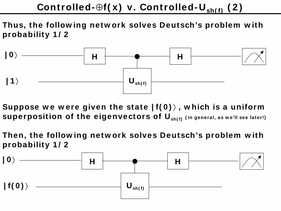
Thus, the following network solves Deutsch’s problem with probability 1/2
Ush(f)
H H|0⟩
|1⟩
Suppose we were given the state |f(0)⟩ , which is a uniform superposition of the eigenvectors of Ush(f) (in general, as we’ll see later!)
Then, the following network solves Deutsch’s problem with probability 1/2
Ush(f)
H H|0⟩
|f(0)⟩

Controlled-⊕f(x) v. Controlled-Ush(f) (3)
Exercise: Compare the states produced by the following networks
Ush(f)
H|0⟩
|f(0)⟩
⊕f(x)
H|0⟩
|0⟩
The equivalence of these two states is the fundamental link between the shift operator (eigenvalue-estimation approach to quantum algorithms) and the controlled-⊕f(x) operator (standard approach)

8-lecture Mini-course in Quantum Computation
Lecture 5
Lawrence Ioannou

Phase Estimation
Ush(f)
H H
|0⟩-|1⟩
|ψ1⟩
|0⟩
|0⟩-|1⟩
|ψ1⟩ = [|0⟩ + (-1)f(0)+f(1)|1⟩](|0⟩-|1⟩)
Let’s rewrite |ψ1⟩ in a more standardised phase notation:
|ψ1⟩ = [|0⟩ + e2πiω|1⟩](|0⟩-|1⟩)
where ω = f(0)⊕f(1)/2
Applying the Hadamard gate to |0⟩+e2πiω|1⟩ gives us |f(0)⊕f(1)⟩ which we will now think of as the most significant bit of the binary expansion of ω:
ω = 0.a1a2a3... ≡ a1/2 + a2/4 + a3/8 + ... (ai∈{0,1})
a1=f(0)⊕f(1), a2=0, a3=0, ...

Phase Estimation (2)ω = 0.a1a2a3 ≡ a1/2 + a2/4 + a3/8 (ai∈{0,1})
This procedure can be generalised to the case where ω has lower-order (nonzero) bits
E.g. suppose ω=0.a1a2a3 i.e. ω=j/8 for some integer j in [0,1,...,7]
Suppose we have prepared the tensor-product state
(|0⟩ + e2πi(4ω)|1⟩) (|0⟩ + e2πi(2ω)|1⟩) (|0⟩ + e2πiω|1⟩)
which, noting e2πi=1, we can also express as
(|0⟩ + e2πi(0.a3)|1⟩) (|0⟩ + e2πi(0.a2a3)|1⟩) (|0⟩ + e2πi(0.a1a2a3)|1⟩)
Our goal is to find a network that will map this state to|a3⟩ |a2⟩ |a1⟩
so that measuring the qubits w.r.t. the computational basis will determine ω

Phase Estimation (3)ω = 0.a1a2a3 ≡ a1/2 + a2/4 + a3/8 (ai∈{0,1})
(|0⟩ + e2πi(0.a3)|1⟩) (|0⟩ + e2πi(0.a
2a
3)|1⟩) (|0⟩ + e2πi(0.a
1a
2a
3)|1⟩) → |a3⟩ |a2⟩ |a1⟩
(we’ll use the facts that H=H-1 and H maps|b⟩ → |0⟩ + (-1)b|1⟩ = |0⟩ + e2πi(0.b)|1⟩ )
We can map the first qubit to |a3⟩ by just applying theHadamard gate, as we did in Deutsch’s problem, to get
|a3⟩ (|0⟩ + e2πi(0.a2a3)|1⟩) (|0⟩ + e2πi(0.a1a2a3)|1⟩)
If the second qubit were in the state |0⟩ + e2πi(0.a2)|1⟩, then we could just apply the Hadamard gate
Note e2πi(0.a2a3) = e2πi(0.0a3)e2πi(0.a2)
= e2πi(a3/4)e2πi(0.a2)
= ei(a3π/2)e2πi(0.a2)
If a3=0, then the second qubit is in the desired state; else, if a3=1, then applying a (-π/2)-phase gate R-π/2 to the secondqubit will give the desired state

Phase Estimation (4)ω = 0.a1a2a3 ≡ a1/2 + a2/4 + a3/8 (ai∈{0,1})
(|0⟩ + e2πi(0.a3)|1⟩) (|0⟩ + e2πi(0.a
2a
3)|1⟩) (|0⟩ + e2πi(0.a
1a
2a
3)|1⟩) → |a3⟩ |a2⟩ |a1⟩
(we use the facts that H=H-1 and H maps|b⟩ → |0⟩ + (-1)b|1⟩ = |0⟩ + e2πi(0.b)|1⟩ )
Because the first qubit is already in the state |a3⟩, we can apply a controlled-R-π/2 gate, to effect the conditional phase-change
Applying this gate and then the Hadamard gate gives
|a3⟩ |a2⟩ (|0⟩ + e2πi(0.a1a2a3)|1⟩)
Similarly (exercise), applying the controlled-R-π/2 gate (to get rid of the e2πi(0.0a20) ) and then the controlled-R-π/4 gate (to get rid of the e2πi(0.00a3) ) gives |a3⟩ |a2⟩ (|0⟩ + e2πi(0.a1)|1⟩), which after a final Hadamard gate gives
|a3⟩ |a2⟩ |a1⟩

Phase Estimation (5)ω = 0.a1a2a3...an ≡ a1/2 + a2/4 +...+ an/2n (ai∈{0,1})
The complete network looks like this
|0⟩ + e2πi(0.a3)|1⟩
|0⟩ + e2πi(0.a2a
3)|1⟩
|0⟩ + e2πi(0.a1a
2a
3)|1⟩
H
H
H
R-π/2
R-π/2 R-π/4
|a3⟩
|a2⟩
|a1⟩
If ω = 0.a1a2a3 ...an, then the obvious generalisation of this network maps
∑−
=
=++++−−
12
0
22)2(2)2(2)2(2 )10)(10()10)(10(21
nnn
x
ixiiii xeeeee ωπωπωπωπωπ L
to
|an⟩ |an-1⟩... |a2⟩ |a1⟩

Phase Estimation (6)(Definition of Quantum Fourier Transform)
ω = 0.a1a2a3...an ≡ a1/2 + a2/4 +...+ an/2n (ai∈{0,1})
∑−
=
=++++−−
12
0
22)2(2)2(2)2(2 )10)(10()10)(10(21
nnn
x
ixiiii xeeeee ωπωπωπωπωπ L
For ω= 0.a1a2a3...an = j/2n, for some j in {0,1,...,2n-1}, the above state is an element of the Fourier basis
Apart from a final reversal of the order of the qubits, the network we described implements the inverse quantum Fourier transform (QFT-1)
For any integer M>1, the quantum Fourier transform, QFT(M), acts on the vector space generated by |0⟩, |1⟩, ..., |M-1⟩, and maps
∑−
=
1
0
2M
x
xMji
xejπ
a

Phase Estimation (7)
jxeM
x
xi a∑−
=
1
0
2 ωπQFT-1: if ω=j/M for j in {0,1,...,M-1}
What about when ω is not j/M for some integer j ?
It turns out that applying QFT-1 to
∑−
=
1
0
2M
x
xi xe ωπ
and measuring w.r.t. the computational basis gives j such thatProb(|j-Mω|≤1) ≥ 8/π2
That is, with high probability, QFT-1 gives the best estimator of ω
Note that increasing M increases the accuracy of the estimate

Eigenvalue EstimationWe can use eigenvalue kick-back and phase estimation (like we did in Deutsch’s problem) to estimate an eigenvalue of a unitary operator U (in Deutsch’s problem we estimated an eigenvalue of the shift operator)
Suppose U is such that
ki
kkeU Ψ=Ψ ωπ2
H
Assume we are given |Ψk⟩ and we can construct a controlled-Ux gate
Then the following network prepares the state ∑−
=
12
0
2n
k
x
xi xe ωπ
Ux|Ψk⟩ |Ψk⟩
|0⟩|0⟩
|0⟩
H
H
nqubits
Applying QFT(2n)-1 to the upper n qubits and measuring w.r.t. the computational basis (and dividing result by 2n) gives the best n-bit estimate of ωk with high probability

Eigenvalue Estimation (2)
Here is a way to effect the controlled-Ux gate, assuming we can construct the controlled-Us gate for s=2i for any i
∑−
=
=++++−−
12
0
22)2(2)2(2)2(2 )10)(10()10)(10(21
nnn
x
ixiiii xeeeee ωπωπωπωπωπ L
Recall
We can build this state one qubit at a time like this
10 )2(2 kiie ωπ+H0
i
U 2kΨ kΨ

Eigenvalue Estimation (3)
H
Ux
|0⟩|0⟩
|0⟩
H
H
∑−
=
Ψ1
0
r
kk
nqubits
∑ ∑−
=
−
=
Ψ⎟⎟⎠
⎞⎜⎜⎝
⎛1
0
12
0
2r
kk
x
xin
k xe ωπ
Of course, if we input an equally-weighted superposition of r eigenvectors in the bottom register, then applying the inverse-QFT to the top n qubits and measuring will give an estimate of a particular ωk with probability 1/r
(Recall that we did this in Deutsch’s problem)

Period-FindingWe can use the QFT to find the period of a function f such that
f: Z {0,1,...,N-1}
f(x) = f(y) ⇔ x-y ∈ rZ
if given the controlled-⊕f(x) gate
⊕f(x)
|x⟩
|y⊕f(x)⟩
|x⟩
|y⟩
Assume a bound on r: M>2r2 (let M=2n, for convenience)
Period-finding algorithm (basic version):
∑−
=
⟩⟩12
0
)(||n
x
xfx1. Using controlled-⊕f(x) (or otherwise!) prepare
2. Apply QFT(2n)-1 to first register
3. Measure first register; result is j
4. (classical) Run continued-fractions algorithm on j/2n to get coprime integers k’ and r’ such that k’/r’ = k/r for some k in {0,1,...,r-1}; test if r’ is period of f; if not, repeat

Period-Finding (2)
There are at least two ways to analyse the algorithm: (1) phase-estimation capability of QFT-1 (due to Kitaev, Mosca et al.)
(2) “classic” properties of QFT (due to Shor)
We’ll cover (1) first, since phase-estimation is fresh in our minds
Consider the shift operator Ush(f) that (perhaps magically) maps
|f(x)⟩ → |f(x+1)⟩
Exercise: verify that
krki
kfsh eU Ψ=Ψπ2
)(where
∑−
=
−=Ψ
1
0
2)(
r
j
rkij
k jfeπ
for k=0,1,...,r-1

Period-Finding (3)
krki
kfsh eU Ψ=Ψπ2
)( ∑−
=
−=Ψ
1
0
2)(
r
j
rkij
k jfeπ
for k=0,1,...,r-1
Estimating a random eigenvalue of Ush(f) allows us to find r:
once a sufficiently accurate estimation of k/r (for some k) is in hand, we give it to the continued-fractions algorithm (described later)
To estimate a k/r, we know that in principle we would need:1. to know how to construct controlled-(Ush(f))x
2. an equally-weighted superposition of |Ψk⟩
However, amazingly, ∑=
=
Ψ=1
0)0(
r
kkf
So, if we could construct controlled-(Ush(f))x , then we coulduse it and |f(0)⟩ in our eigenvalue estimation procedure, in which we would produce the state
∑ ∑−
=
−
=
Ψ⎟⎟⎠
⎞⎜⎜⎝
⎛1
0
12
0
2r
kk
x
xrki
n
xeπ
....

Period-Finding (4)
krki
kfsh eU Ψ=Ψπ2
)( ∑−
=
−=Ψ
1
0
2)(
r
j
rkij
k jfeπ
for k=0,1,...,r-1
∑=
=
Ψ=1
0)0(
r
kkf
But clearly, applying the controlled-(Ush(f))x to
)0(12
0fx
n
x∑−
=gives
∑−
=
⟩⟩12
0
)(||n
x
xfx = ∑ ∑−
=
−
=
Ψ⎟⎟⎠
⎞⎜⎜⎝
⎛1
0
12
0
2r
kk
x
xrki
n
xeπ
Thus, we can make the “eigenvalue-estimation state”
∑ ∑−
=
−
=
Ψ⎟⎟⎠
⎞⎜⎜⎝
⎛1
0
12
0
2r
kk
x
xrki
n
xeπ
by just using the given controlled-⊕f(x) gate
Measuring the first register of the above state will give us an estimate x/2n of k/r

Period-Finding (5)we have an estimate x/M of k/r, where M>2r2 and M= 2n
Every real number y has a sequence of rationals, calledconvergents, that approximate it
Lemma: Given the integers x and M, if
2211rMM
xrk
<≤−
then the fraction k/r is a convergent of x/M
With high probability, we know our x/M satisfies the first inequality; the second inequality is satisfied by assumption
The continued fractions algorithm (see next slide) is used to compute the convergents of x/M, and finds coprime integers k’ and r’ such that k’/r’=k/r; we test r’ to see if it is r
k and r are coprime with reasonably high probability, so the given period-finding algorithm terminates quickly (there are more sophisticated ways to increase success probability)

Period-Finding (6)
Define [ ]
L
L
a
aa
aaa
11
11,,
2
1
00
++
++≡
O
K
where the are positive integers (except may be 0)ia 0a
Define the mth convergent (0≤m≤L) to this continued fraction to be [ ]maa ,,0 K
We give x/M to the continued fractions algorithm, and it computes the convergents of x/M
This is an efficient computation (terminates quickly)

Period-Finding (7)
Applying the continued fractions algorithm to 31/13
211
11
12
12
2311
12
12
321
12
12
3512
12
532
12
51312
1352
1331
++
++=
++
+=
++
+=
++=
++=
+=+=Notice the “split-and-invert” nature of the algorithm
(Example taken from Nielsen and Chuang)
STOP when you get a 1 in the numerator after splitting

Period-Finding (8) (a la Shor)
Let us briefly look at Shor’s original analysis of the period-finding algorithm
First let’s modify the algorithm to be like Shor’s original algorithm, using QFT(2n) instead of QFT(2n)-1 :
Quantum part of period-finding algorithm (basic version):
1. Using controlled-⊕f(x) (or otherwise!) prepare
2. Apply QFT(2n) to first register
∑−
=
⟩⟩12
0
)(||n
x
xfx
3. Measure first register; result is j
So as not to panic, note that QFT=QFT-1QFT2, so we can think of this revised period-finding algorithm as the previous one, but with an extra QFT2 after the QFT-1
Exercise: show that QFT(M)2 is a fairly benign operation mapping |j⟩ |M-j mod M⟩

Period-Finding (9) (a la Shor)
The Fourier transform is well known in mathematics and physics to pick out the frequency of a periodic function
Similarly, the QFT would map a periodic superposition of computational basis states to a state that had most probability amplitude in basis states corresponding to the period
For convenience, assume 2n = tr for some integer t (obviously this would rarely be the case; when it’s not, as long as 2n/r is sufficiently big, the end result will be approximately the same...)
∑ ∑∑−
=
−
=
−
=⎟⎟⎠
⎞⎜⎜⎝
⎛+=⟩⟩
1
0
1
0
12
0)()(||
r
l
t
jxlfjrlxfx
n
periodic superposition!

Period-Finding (10) (a la Shor)For convenience, assume 2n = tr for some integer t
To simplify notation, assume we’ve measured the second register, thus leaving the first register in the state
∑−
=
+1
0
t
jjrl (for some l)
(note this measurement is optional; it does not change the algorithm)Applying QFT(2n) now gives
xeen
nn
x
t
j
xijrilx∑ ∑−
=
−
=⎟⎟⎠
⎞⎜⎜⎝
⎛12
0
1
0
222/2 ππ
When x/2n = k/r, the sum inside the brackets is equal to t; otherwise, the sum is 0 (if 2n ≠ tr, the sums are approximately t and 0)
Thus measuring this state w.r.t. the computational basis gives an estimate of k/r for some k (just like the eigenvalue-estimation analysis did)

Order-Finding
For positive coprime integers N and y, the order of y modulo N is defined to be the least positive integer r such that
yr≡1 (mod N)
The INTEGER FACTORING problem reduces to the order-finding problem
We can use the period-finding algorithm to solve the order-finding problem, noting that the order of y is the period of the function
f(x)=yx
Note that for this particular f(x) we do know how to implement the shift operator: just multiply f(x) by y to get f(x+1)

8-lecture Mini-course in Quantum Computation
Lecture 6
Lawrence Ioannou

Reduction of Factoring to Order-Finding
The (probabilistic) reduction-algorithm is as follows:
FindFactor(N)
1. If N is even, return factor 2
2. Determine if N=cb; if so, return factor c
3. Randomly choose y from ZN*; if gcd(y,N)>1, return factor gcd(y,N)
4. Find the order r of y modulo N
5. If r is even, compute d=gcd(yr/2-1,N), return d if d≠1; else go to step 3

Reduction of Factoring to Order-Finding (2)FindFactor(N)3. Randomly choose y from ZN*; if gcd(y,N)>1, return factor gcd(y,N)4. Find the order r of y modulo N5. If r is even, compute d=gcd(yr/2-1,N), return d if d≠1; else go to step 3
We give a proof for when N=pq, for p and q prime:
Let y1 and y2 be generators of Zp* and Zq* respectively
Note that randomly choosing y from ZN* is equivalent to randomly choosing x1 from Zp* and x2 from Zq*, and then computing y as the (unique) solution to the congruence system y ≡ y1
x1 (mod p)y ≡ y2
x2 (mod q)(using the Chinese Remainder Theorem)
The order of y modulo p is r1 = (p-1)/gcd(x1,p-1)The order of y modulo q is r2 = (q-1)/gcd(x2,q-1)The order of y modulo N is r = lcm(r1,r2) = r1r2/gcd(r1,r2)
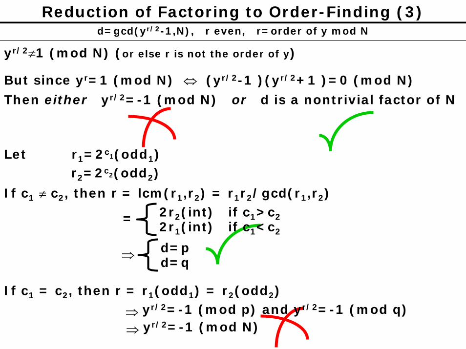
Reduction of Factoring to Order-Finding (3)d=gcd(yr/2-1,N), r even, r=order of y mod N
yr/2≠1 (mod N) (or else r is not the order of y)
Then either yr/2=-1 (mod N) or d is a nontrivial factor of NBut since yr=1 (mod N) ⇔ (yr/2-1 )(yr/2+1 )=0 (mod N)
Let r1=2c1(odd1)r2=2c2(odd2)
If c1 ≠ c2, then r = lcm(r1,r2) = r1r2/gcd(r1,r2)
= 2r2(int) if c1>c22r1(int) if c1<c2
⇒ d=pd=q
If c1 = c2, then r = r1(odd1) = r2(odd2)
⇒ yr/2=-1 (mod p) and yr/2=-1 (mod q) ⇒ yr/2=-1 (mod N)

Reduction of Factoring to Order-Finding (4)
r1=2c1(odd1)r2=2c2(odd2)
y1 and y2 are generators of Zp* and Zq* respectively
Thus c1 ≠ c2 is success and c1 = c2 is failure
What’s the probability that c1 ≠ c2 ?
Suppose p-1=2k1s1 and q-1=2k2s2
We only explain the worst case k1=k2=1 (y1, y2 have order 2s):
The even powers yixi of yi have odd order ri
Whereas the odd powers have order 2(oddi)
Thus if xi are chosen randomly, Prob(c1 ≠ c2) =1/2 (because there are just as many even xi as there are odd xi)

Breaking the RSA CryptosystemOld-school cryptosystems used a symmetric or secret key
Two parties (Alice and Bob) wishing to communicate secretly would first (somehow) decide on a random binary string (the secret key)
Before quantum key distribution, this was very impractical
In the 1970s, people had the idea of using complexity-theoretic assumptions to build computationally-securecryptosystems (like the RSA cryptosystem)
These cryptosystems use a public key (chosen by Alice), allowing anyone to send Alice a secret message without ever sharing a secret in the first place – the public key is good for many messages
Of course, given enough time, the public key can be used to break the cryptosystem
The assumption of the RSA cryptosystem is that the integer-factorisation problem is very difficult (not in BPP)

Breaking the RSA Cryptosystem (2)The RSA cryptosystem (for anyone to send secret messages to Alice):
Alice
Chooses two large primes p,q
Computes N=pq
Chooses small odd integer e, where gcd(e,ϕ(N))=1, ϕ(N)=(p-1)(q-1)
Computes d ≡ e-1 mod ϕ(N)
Publishes: Public Key = (N,e)
Keeps secret: Private Key = (N,d)
EvaBob DougCharlie
Clearly, knowing the factors p,q of N allows anyone to compute the private key d

Breaking the RSA Cryptosystem (3)
For completeness, we give the encryption and decryption algorithms:
To encrypt and send a message m ∈ {0,1,...,N-1}, Bob computes and sends the number c=me (mod N)
To decrypt the received ciphertext c, Alice computescd mod N = med mod N
= m1+kϕ(N) mod N
If gcd(m,N)=1, then Euler’s generalisation of Fermat’s Little Theorem gives mkϕ(N) mod N = 1, and thus the decryption is successful
Exercise: When m and N=pq have a common factor, then cd
mod N still equals m (use the Chinese Remainder Theorem)
Exercise: Show how to compute m from c using an order-finding algorithm without factoring N

Discrete Logarithm ProblemNot all public-key cryptosystems are based on the classical difficulty of factoring
The El Gamal public-key cryptosystem is based on the classical difficulty of the discrete logarithm problem (DLP):
Let p be a prime, α∈Zp* a generator, and β∈Zp*.
Find unique integer s such that β ≡ αs (mod p)
Classically, this problem is thought to be hard for well-chosen p (p should have at least 150 digits and p-1 should have at least one large prime)
To set up the El Gamal cryptosystem, Alice chooses well the above parameters, publishes the public key (p, α, β) but keeps the private key s secret
If Bob wants to send a message m, he chooses a random k ∈Zp-1 , and sends to Alice (y1, y2) = (αk mod p, mβk mod p)
To decrypt, Alice computes m= y2(y1s)-1 mod p (Exercise: verify)

Discrete Logarithm Problem (2)
We can define the DLP more generally, in any group:
Given elements α and β=αs, s∈{0,1,...,r-1} (r is the order of α), from the group H, find s
Note that we can reduce the DLP to period-finding:
The functionf(x1, x2) = αsx1+x2 = αx2 βx1
is periodic, with period (1, -s)
From the period, we can calculate the discrete logarithm s, and thus we can break the El Gamal cryptosystem with a quantum computer
To do this, we use a straightforward modification of the period-finding algorithm, noting that the domain of f is now 2-dimensional...

Discrete Logarithm Problem (3)Let p be a prime, α∈Zp* a generator, and β∈Zp*.
Find unique integer s such that β ≡ αs (mod p)
The algorithm can be thought of as estimating eigenvaluese2πik/r and e2πiks/r of the “shift” operators Uα: |y⟩ |αy⟩ and Uβ : |y⟩ |βy⟩, where r is the order modulo p of α (which we can compute using the order-finding algorithm)
Since we know r, we just need to estimate the eigenvalueswith an error of at most 1/2r to find the numerators k and ks(we don’t need the continued-fractions algorithm)
Finally, from k and ks, s is calculated as s = k-1(ks) mod r
Uαx
|0⟩
|0⟩ H⊗n
H⊗n
Uβx
QFT-1
QFT-1
(2n>2r)
∑−
=
Ψ1
0
r
kk

Quantum Cryptography
We’ve seen that explioting quantum mechanics allows us to crack some (but not all!) classical public-key cryptosystems
But it also allows us to build new, unconditionally-securecryptographic protocols
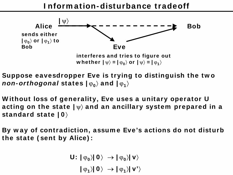
Information-disturbance tradeoff
Suppose eavesdropper Eve is trying to distinguish the two non-orthogonal states |ϕ0⟩ and |ϕ1⟩
Without loss of generality, Eve uses a unitary operator U acting on the state |ψ⟩ and an ancillary system prepared in a standard state |0⟩
Alice Bob
Eve
|ψ⟩
sends either |ϕ0⟩ or |ϕ1⟩ to Bob
interferes and tries to figure out whether |ψ⟩ =|ϕ0⟩ or |ψ⟩ =|ϕ1⟩
By way of contradiction, assume Eve’s actions do not disturb the state (sent by Alice):
U: |ϕ0⟩|0⟩ → |ϕ0⟩|v⟩
|ϕ1⟩|0⟩ → |ϕ1⟩|v’⟩

Information-disturbance tradeoff (2)
Eve would like to measure the second register, in order to identify (or at least get some information about) the state in the first register
Thus she needs |v⟩ and |v’⟩ to be different
But the unitarity of U (along with the non-orthogonality of |ϕ0⟩and |ϕ1⟩) implies that |v⟩ and |v’⟩ are identical
Thus Eve can’t distinguish the states, unless she disturbs at least one of them
Alice Bobsends either |ϕ0⟩ or |ϕ1⟩ to Bob Eve
|ψ⟩
interferes and tries to figure out whether |ψ⟩ =|ϕ0⟩ or |ψ⟩ =|ϕ1⟩
U: |ϕ0⟩|0⟩ → |ϕ0⟩|v⟩|ϕ1⟩|0⟩ → |ϕ1⟩|v’⟩

Information-disturbance tradeoff (3)
Proposition [12.18 in textbook]: In any attempt to distinguish between two non-orthogonal quantum states, information gain is only possible at the expense of introducing disturbance to the signal
The above theorem is at the heart of quantum key distribution (QKD)
Alice can send quantum states to Bob, and an eavesdropper will not learn much about the states unless she disturbs them – in which case (one can show that) Alice and Bob could detect Eve’s meddling

Quantum Key Distribution (QKD)
Alice Bob|ψ⟩
Eve
sends either |ϕ0⟩ or |ϕ1⟩ to Bob
H|0⟩
|0⟩
|1⟩
H|1⟩
Define |ϕ0⟩ := |0⟩|ϕ1⟩ := (|0⟩+|1⟩)/√2 = H|0⟩
For each secret bit, a∈{0,1}, chosen by Alice:
1. Alice sends |ψ⟩=|ϕa⟩ to Bob
2. Bob chooses random bit, a’∈{0,1}, and measures |ψ⟩ w.r.t. {Ha’|0⟩, Ha’|1⟩}, obtaining result b∈{0,1} (w.r.t. basis ordering)
3. Bob publicly announces b, but keeps a’ secret; Alice and Bob keep a and a’ only if b=1 (else discard this a and a’)Note: If a=a’, then b=0; else if a=1-a’, then b is randomly 0 or 1. Thus about ¾ of the {a,a’} are discarded
4. The final shared key bit is: a (for Alice) and 1-a’ (for Bob)
Alice and Bob then (publicly) choose a sufficiently large proportion of the bits to check to see if they are the same; they abort if too many bits are different.

Quantum Key Distribution (2)
H|0⟩
|0⟩
|1⟩
H|1⟩
Alice
Bob
a=0
a=1
a’=0
a’=1
a’=1
a’=0
Measurement result
0 (a=a’)
0 or 1 randomly (a=1-a’)
0 or 1 randomly (a=1-a’)
0 (a=a’)

Quantum Key Distribution (3)
The protocol based on the previous two slides is known as B92, after Bennett, who discovered this streamlining of his original protocol known as BB84 (after Bennett and Brassard)
Note we have not shown that the protocol is secure (or even described the whole protocol), but it should be clear that Eve learns nothing useful from the public discussion alone. A security proof would involve showing that if Eve did try to measure the states |ψ⟩=|ϕa⟩, she would disturb them such that Alice’s and Bob’s final shared key would fail the check at the end
There is another, fundamentally different type of protocol, called E91, discovered by Ekert; it uses EPR pairs
|β00⟩ =|00⟩ + |11⟩

Quantum Key Distribution (4)
Define |+⟩ = H|0⟩|-⟩ = H|1⟩
Note (ignoring normalisation factors)
|0⟩|0⟩ + |1⟩|1⟩ = |+⟩|+⟩ + |-⟩|-⟩
If Alice and Bob share this state (Alice has the left qubit and Bob has the right qubit), and they both measure their qubits with respect to the same basis, either {|0⟩, |1⟩} or {|+⟩, |-⟩}, then they must get the same result (0 or 1 as in the B92 protocol description)
Exercise: Derive the E91 protocol (to the same level of detail that we described B92; assuming the “shared EPR pairs” are perfect and perfectly shared, you don’t need to have a test of the shared key bits at the end; in the full E91 protocol, Alice and Bob can test (using the public channel) the fidelity of their EPR pairs at the beginning of the protocol to ensure they are sharing actual EPR pairs to a sufficiently high fidelity)
Note that all the QKD protocols rely on the existence of an authenticated public channel

8-lecture Mini-course in Quantum Computation
Lecture 7
Lawrence Ioannou

Unordered-Search Problem
Given black box for f: {0,1}n → {0,1}
Find an x such that f(x)=1 (we are promised such x exists)
(think of {0,1}n as a “database”, perhaps...)
The best classical algorithm for unordered search requires roughly N=2n queries of f
The best quantum algorithm (due to Lov Grover) for unordered search requires roughly N1/2=2n/2 queries of f (we won’t show optimality today)
We assume we are given a quantum black box
(n qubits)
⊕f(x)
|x⟩
|y⊕f(x)⟩
|x⟩
|y⟩(1 qubit)

Unordered-Search Problem (2)
⊕f(x)
|x⟩
|y⊕f(x)⟩
|x⟩
|y⟩
What shall we do with this black box?
Inspired by Deutsch’s algorithm, we notice that
⊕f(x)
|x⟩ (-1)f(x)|x⟩
|0⟩ -|1⟩ |0⟩ -|1⟩
|ψ1⟩
|ψ1⟩ = |x⟩ ⊗ (|f(x)⟩ -|1 ⊕f(x)⟩)
=|x⟩ ⊗ (|0⟩ -|1⟩) if f(x)=0|x⟩ ⊗ (|1⟩ -|0⟩) if f(x)=1
= (-1)f(x)|x⟩ ⊗ (|0⟩ -|1⟩)

Unordered-Search Problem (3)
⊕f(x)
|x⟩ (-1)f(x)|x⟩
|0⟩ -|1⟩ |0⟩ -|1⟩ (ancillary qubit)
So we use the black box to implement an operator Uf mapping
Uf : |x⟩ (-1)f(x)|x⟩
Recall we can use the n-qubit Hadamard gate, H⊗n, to make the equally-weighted superposition of all computational basis states: H
( ) ∑∈
⊗ =+nx
n x}1,0{
10|0⟩|0⟩
|0⟩
H
H
nqubits
|0⟩+|1⟩
|0⟩+|1⟩
|0⟩+|1⟩
Let |Y⟩ be this state:
∑∑−
=∈
⊗ ≡=≡Υ12
0}1,0{
0n
n ix
n ixH Recall there are two summation conventions: we can label the computational basis states by binary strings (x) or the corresponding integers (i)

Unordered-Search Problem (4)
∑−
=
⊗ =≡Υ12
00
n
i
n iH
Note |Y⟩ is just a basis state of another basis called theHadamard basis which is
{H⊗n|x⟩ : x∈{0,1}n}
(i.e. the Hadamard basis is the basis derived from applying the Hadamardgate to the elements of the computational basis)
Let |x*⟩ ≡ H⊗n|x⟩ for x∈{0,1}n denote an element in theHadamard basis (similarly |i*⟩ ≡ H⊗n|i⟩ for i∈{0,1,...,2n-1})
Computational basis = {|x⟩ : x∈{0,1}n}
Hadamard basis = {|x*⟩ : x∈{0,1}n}
Note |Y⟩ = |0*⟩

Unordered-Search Problem (5)
*0012
0==≡Υ ∑
−
=
⊗n
i
n iH
Computational basis = {|x⟩ : x∈{0,1}n} = {|i⟩ : i=0,1,...,2n-1}Hadamard basis = {|x*⟩ : x∈{0,1}n} = {|i*⟩ : i=0,1,...,2n-1}
Introduce the operator U0 that maps
U0: |0⟩ -|0⟩
|i⟩ |i⟩ for i ≠ 0
Consider the operator UY ≡ H⊗nU0H⊗n, which does the analogous operation in the Hadamard basis:
UY|Y⟩ = - |Y⟩
UY|i*⟩ = |i*⟩ for i ≠ 0
since UY|i*⟩ = H⊗nU0H⊗n H⊗n|i⟩
= H⊗nU0|i⟩, because H⊗n is its own inverse

Unordered-Search Problem (6)But what does the operator UY ≡ H⊗nU0H⊗n do in the computational basis?
Recall that the (vector) projection of a unit-vector |v⟩ onto a unit-vector |u⟩ is given by
(|u⟩,|v⟩)|u⟩
where (|u⟩,|v⟩) is the inner product of the two vectors (like dot-product in a Euclidean space)
We will write (|u⟩,|v⟩) as ⟨u|v⟩ (this is actually quantum-mechanical shorthand for
the product ⟨u||v⟩ where ⟨u| is the dual-vector of |u⟩)
Let P|u⟩ be the (linear) projection operator, projecting onto |u⟩
P|u⟩ |v⟩ = ⟨u|v⟩ |u⟩

Unordered-Search Problem (7)Action of UY ≡ H⊗nU0H⊗n in the computational basis
P|u⟩ |v⟩ = ⟨u|v⟩ |u⟩
( )Υ
⊗⊗
⊗⊗
⊗⊗⊗⊗Υ
−=
−=
⎟⎟⎟⎟⎟
⎠
⎞
⎜⎜⎜⎜⎜
⎝
⎛
⎥⎥⎥⎥
⎦
⎤
⎢⎢⎢⎢
⎣
⎡
−
⎥⎥⎥⎥
⎦
⎤
⎢⎢⎢⎢
⎣
⎡
=
⎥⎥⎥⎥
⎦
⎤
⎢⎢⎢⎢
⎣
⎡−
==
PI
HPIH
HH
HHHUHU
nn
nn
nnnn
2
2
00000
000001
2
10000
010001
10000
010001
0
0
L
OM
M
L
L
OM
M
L
L
OM
M
L

Unordered-Search Problem (8)Action of UY ≡ H⊗nU0H⊗n in the computational basis
N=2nP|u⟩ |v⟩ = ⟨u|v⟩ |u⟩
Thus -UY = 2P|Y⟩ -I
Consider an arbitrary state of an n-qubit register∑−
=
1
0
N
kk kα
where N=2n
kiN
iN
ki
Nk
kkPkP
N
k
N
i
N
k
k
N
i
N
k
kN
k
N
ik
N
kk
N
kk
N
kk
∑∑ ∑
∑ ∑∑ ∑
∑∑∑
−
=
−
=
−
=
−
=
−
=
−
=
−
=
−
=
−
=Υ
−
=Υ
=⎟⎠
⎞⎜⎝
⎛=
⎟⎟⎠
⎞⎜⎜⎝
⎛ Υ=⎟
⎠
⎞⎜⎝
⎛Υ=
ΥΥ==
1
0
1
0
1
0
1
0
1
0
1
0
1
0
1
0
1
0
1
0
1
αα
αα
ααα
where ⟨α⟩ is the mean average of all the αk

Unordered-Search Problem (9)Action of UY ≡ H⊗nU0H⊗n in the computational basis
N=2nP|u⟩ |v⟩ = ⟨u|v⟩ |u⟩
Thus -UY = 2P|Y⟩ -I maps the arbitrary state
∑−
=
1
0
N
kk kα
to
[ ]∑−
=
+−1
02
N
kk kαα
-UY is sometimes referred to as the inversion about the mean:
∑−
=
=1
0
1 N
kkN
αα (the mean average)

Unordered-Search Problem (10)
Uf : |x⟩ (-1)f(x)|x⟩
∑−
=
1
0
N
kk kα [ ]∑
−
=
+−1
02
N
kk kαα-UY:
The quantum searching algorithm is
1. Prepare an n-qubit register in the state |Y⟩=∑−
=
12
0
n
ii
2. Apply the operator G ≡ -UY Uf roughly N1/2 times
3. Measure the register; output is x such that f(x)=1 with high probability
We’ll give a high-level analysis first, using the inversion-about-the-mean interpretation, then we’ll give a more rigorous analysis using analysis

Unordered-Search Problem (11)
Uf : |x⟩ (-1)f(x)|x⟩ ∑−
=
1
0
N
kk kα [ ]∑
−
=
+−1
02
N
kk kαα-UY:
G ≡ -UY Uf
Suppose, for simplicity, f(x)=1 for only one element x
It suffices to see what the effect of G is on the starting state(it’s clear that continuing to apply G will produce the desired effect):
∑
∑∑
∈
∈Υ
∈
⎟⎟⎠
⎞⎜⎜⎝
⎛+
−−≈
−−=
n
nn
x
xf
x
xf
x
xNN
xN
UxN
G
}1,0{
)(
}1,0{
)(
}1,0{
12)1(
)1(1
approx. mean avg.
Thus the amplitude of the solution state increased to roughly 3/N1/2, whereas the amplitude of the other states slightly decreased

Unordered-Search Problem (12)
Uf : |x⟩ (-1)f(x)|x⟩ G ≡ -UY Uf
Let’s proceed with a more rigorous analysis of the algorithm
We can assume that f(x)=1 has more than one solution
Let X1 be the set of solutions to f(x)=1 (the good x’s)Let X0 be the set of solutions to f(x)=0 (the bad x’s)
Define the equally-weighted superpositions of the “good” and “bad” states:
∑
∑
∈
∈
=
=
0
1
00
11
1Xx
Xx
xX
X
xX
X 1
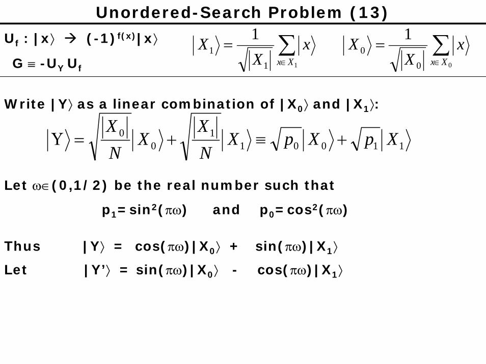
Unordered-Search Problem (13)
∑∈
=11
11
Xxx
XX ∑
∈
=00
01
Xxx
XXUf : |x⟩ (-1)f(x)|x⟩
G ≡ -UY Uf
Write |Y⟩ as a linear combination of |X0⟩ and |X1⟩:
110011
00 XpXpX
NX
XNX
+≡+=Υ
Let ω∈(0,1/2) be the real number such that
p1=sin2(πω) and p0=cos2(πω)
Thus |Y⟩ = cos(πω)|X0⟩ + sin(πω)|X1⟩
Let |Y’⟩ = sin(πω)|X0⟩ - cos(πω)|X1⟩

Unordered-Search Problem (14)
Uf : |x⟩ (-1)f(x)|x⟩ |Y⟩ = cos(πω)|X0⟩ + sin(πω)|X1⟩|Y’⟩ = sin(πω)|X0⟩ - cos(πω)|X1⟩G ≡ -UY Uf
We now have two (orthonormal) bases for the same 2-dimensional subspace:
{|X0⟩, |X1⟩} and {|Y⟩, |Y’⟩}(Note Uf and –UY are reflections in this plane, changing the sign of one coordinate)
We analyse the action of G=-UYUf using these two bases
Let |Ψ⟩ = cos(ϕ)|X0⟩ + sin(ϕ)|X1⟩ be any state
Uf|Ψ⟩ = cos(ϕ)|X0⟩ - sin(ϕ)|X1⟩= cos(ϕ+πω)|Y⟩ + sin(ϕ+πω)|Y’⟩ (switch to basis {|Y⟩, |Y’⟩}
to apply -UY)G|Ψ⟩ = cos(ϕ+πω)|Y⟩ - sin(ϕ+πω)|Y’⟩
= cos(ϕ+2πω)|X0⟩ + sin(ϕ+2πω)|X1⟩
Thus G (the product of two reflections) gives us a rotation of 2πω in the plane spanned by |X0⟩ and |X1⟩

Unordered-Search Problem (15)G: cos(ϕ)|X0⟩ + sin(ϕ)|X1⟩ cos(ϕ+2πω)|X0⟩ - sin(ϕ+2πω)|X1⟩
Since the search algorithm starts in the state with ϕ=πω, we see that after k applications of G, the state of the n-qubitregister is
cos((2k+1)πω)|X0⟩ + sin((2k+1)πω)|X1⟩
To measure a good state, we want sin((2k+1)πω) ~ 1
This is true when k ~ 1/(4ω) - 1/2
~ π/[4(p1)1/2]
= π/[4(|X1|/N)1/2]
= πN1/2/[4(|X1|)1/2]
Thus applying G πN1/2/[4(|X1|)1/2] times gives a state with large probability amplitude in the state |X1⟩

Unordered-Search Problem (16)The operator G, also called the Grover iterate, has eigenvectors in the 2-dimensional space
10 221 XiX +=Ψ+
10 221 XiX −=Ψ−
with respective eigenvalues e2πiω and e-2πiω
The initial state |Y⟩ = cos(πω)|X0⟩ + sin(πω)|X1⟩ is expressed in this eigenbasis as
−
−
+ Ψ+Ψ22
ωπωπ ii ee
Thus applying Gk to this state gives
−
+−
+
+
Ψ+Ψ22
)12()12( ωπωπ kiki ee
This gives an alternative derivation of the number k of required applications of G in the search algorithm
CountingG = -UY Uf has eigenvalues e2πiω and e-2πiω
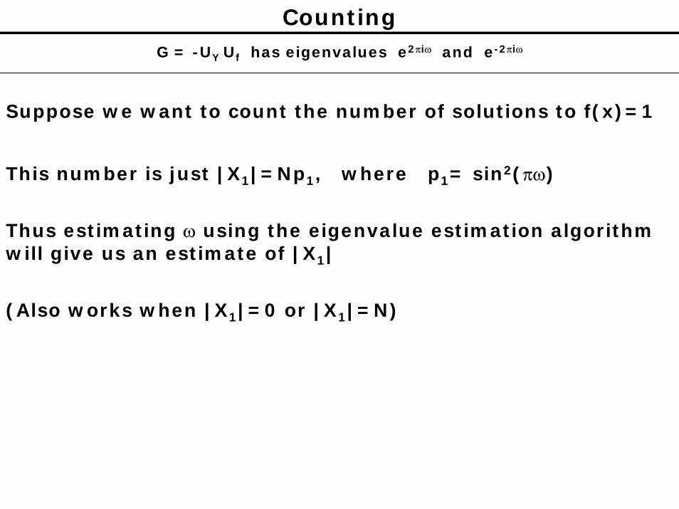
Suppose we want to count the number of solutions to f(x)=1
This number is just |X1|=Np1, where p1= sin2(πω)
Thus estimating ω using the eigenvalue estimation algorithm will give us an estimate of |X1|
(Also works when |X1|=0 or |X1|=N)

8-lecture Mini-course in Quantum Computation
Lecture 8
Lawrence Ioannou

Review of n-qubit Hadamard Gate, H⊗n
Recall the one-qubit Hadamard gate, H, maps
⎥⎦
⎤⎢⎣
⎡−1111
21
H: |0⟩ (|0⟩ + |1⟩)/21/2
|1⟩ (|0⟩ - |1⟩)/21/2 the matrix-representation, with respect to the computational basis, of the Hadamard gate
Alternatively
H: |b⟩ (|0⟩ + (-1)b|1⟩)/21/2, for b∈{0,1}
which can also be written
H: |b⟩ (Σx(-1)b⋅x|x⟩)/21/2, for b,x∈{0,1}
Exercise: show that the n-qubit Hadamard gate, H⊗n, maps
∑∈
•⊗ −nx
yxn xN
yH}1,0{
)1(1: a
where x•y = Σi xiyi, where x=xn-1xn-2...x1x0∈{0,1}n and similarly for y

Measurement as a vector-projection
Recall P|u⟩ is the (linear) projection operator, projecting onto the vector |u⟩:
P|u⟩ |v⟩ = ⟨u|v⟩ |u⟩
inner product of vector |u⟩ and vector |v⟩
A measurement of the n-qubit state
with respect to the computational basis can be thought of as applying (to |ψ⟩) the projection operator P|x⟩ with probability αx (and then renormalising P|x⟩|ψ⟩ so it’s a unit-vector still)
∑∈
=nx
x x}1,0{
αψ
|ψ⟩
is equivalent to
|ψ⟩P|x⟩w.p. |αx|2
|x⟩ w.p. |αx|2
|x⟩
(Note “w.p.” is shorthand for “with probability”)
Measurement as a vector-projection (2)
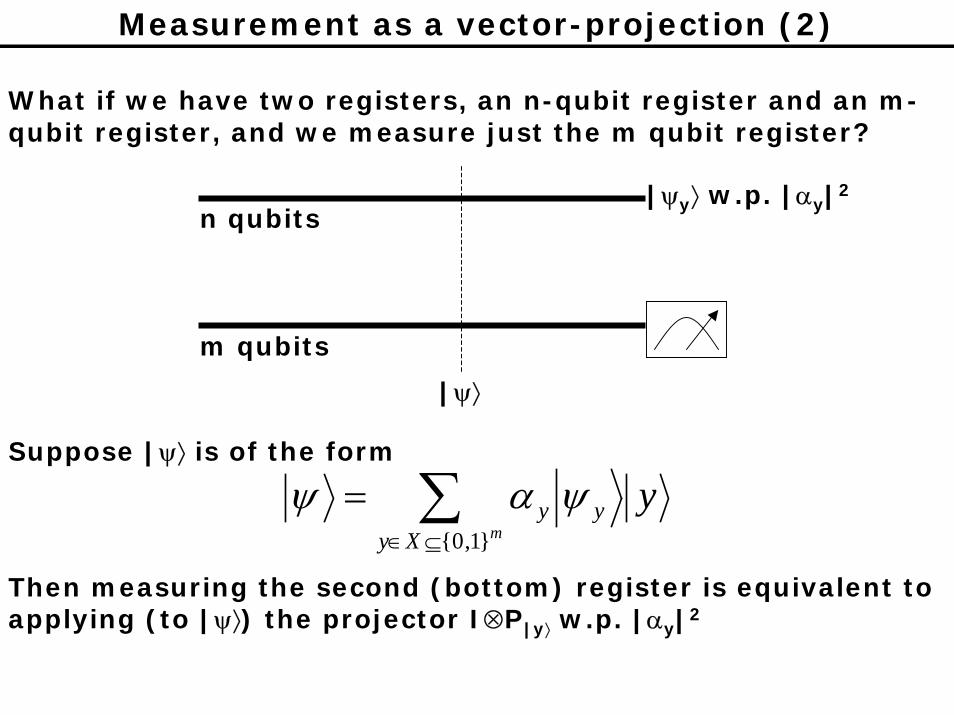
What if we have two registers, an n-qubit register and an m-qubit register, and we measure just the m qubit register?
|ψ⟩
n qubits
m qubits
|ψy⟩ w.p. |αy|2
Suppose |ψ⟩ is of the form
∑⊆∈
=mXy
yy y}1,0{
ψαψ
Then measuring the second (bottom) register is equivalent to applying (to |ψ⟩) the projector I⊗P|y⟩ w.p. |αy|2

Measurement as a vector-projection (3)
n qubits
m qubits
∑⊆∈
=mXy
yy y}1,0{
ψαψ
|ψy⟩ w.p. |αy|2
(this is actually known as a mixed state – a probabilistic distribution of pure states)
Note that if we did not actually do the measurement, but just ignored (or threw away, or traced out) the second (bottom) register, then we can just think of the first (upper) register as in the state |ψy⟩ w.p. |αy|2
Sometimes, to make notation simpler, we ignore the bottom register after some point in the computation or (equivalently) assume that we have measured it

Simon’s problem
Given a black box which computes the function
f(x)=f(x⊕s), for some s ∈ {0,1}n
f: {0,1}n → {0,1}n such that
Find the “period” s
Example (taken from Artur Ekert’s course notes):
x f(x)
000 111001 010010 100011 110100 100101 110110 111111 010
s=110 is the period (in the additive group (Z2)3)
f(x ⊕ 110) = f(x)
f(000) = f(000 ⊕ 110) = f(110) =111f(001) = f(001 ⊕ 110) = f(111) =010f(010) = f(010 ⊕ 110) = f(100) =100f(011) = f(011 ⊕ 110) = f(101) =110

Simon’s problem (2)Given a black box which computes the function
f: {0,1}n → {0,1}n such thatf(x)=f(x⊕s), for some s ∈ {0,1}n
Find the “period” s
⊕f(x)
H⊗n H⊗nn qubits
n qubits
|0⟩
|0⟩
|ψ1⟩ |ψ2⟩
( ) )(
)()(
0)()(
00
0}1,0{ )()( )()(:
1
0
0 0
xfsxx
xfxxfx
fRangexf
x fRangexf xfxfxn
∑
∑ ∑ ∑
∈
∈ ∈ =
⊕+=
⎟⎟⎠
⎞⎜⎜⎝
⎛==ψ
(optional measurement/discarding – just for convenience of analysis)
( ) ∑ ••⊗ −+−=⊕+=y
ysxyn ysxxH ])1(1[)1( 0002ψ

Simon’s problem (3)Given a black box which computes the function
f: {0,1}n → {0,1}n such thatf(x)=f(x⊕s), for some s ∈ {0,1}n
Find the “period” s
⊕f(x)
H⊗n H⊗n|0⟩n qubits |y⟩such that s•y=0
|0⟩n qubits
Thus we effectively end up measuring the state
∑ •• −+−y
ysxy y])1(1[)1( 0
Note that the probabililty amplitude of |y⟩ such that s•y=1 is 0
Thus the result of the measurement is a particular y such that s•y=0, with probability 2/2n

Simon’s problem (4)Given a black box which computes the function
f: {0,1}n → {0,1}n such thatf(x)=f(x⊕s), for some s ∈ {0,1}n
Find the “period” s
Simon’s algorithm is to repeat the previous experiment roughly n times to get a linearly independent set y(1), y(2), ..., y(n) such that y(i)•s=0 (the probability of failing to produce a linearly independent set is
less than 0.75)
Then we can solve for s by solving the system of n linear equations:
y(1)•s=0y(2)•s=0
y(n)•s=0
•••
It may help to think of each equation y(i)•s=0 as
01)(11
)(10
)(0 =+++ −− n
in
ii sysysy Lwhere the si are the n “unknowns”

Hidden Subgroup Problem (HSP)
The problems studied so far are special cases of the more general hidden subgroup problem:
Let f be a function from a finitely generated group G to a finite set X, such that
(i) f is constant on cosets of a subgroup K and
(ii) f is distinct on each coset.
Given the controlled-⊕f(x) gate, find a generating set for K
The idea is that the function f is “hiding” the subgroup K

HSP (2)
We need the group to be Abelian (so that it is a product of cyclic groups)
K
g1+K
g2+K
g3+K
f(0)
f(1)
f(2)
f(3)
gi+K denotes a coset of K

HSP (3)
Here are the problems we have studied, a la HSP:
Deutch’s problem:f: {0,1} {0,1}
f(x)=f(y) iff x-y∈K, where eitherK={0} or K={0,1}
Period-Finding:f: Z any finite set
f(x)=f(y) iff x-y∈K, where
K=rZ
Discrete Logarithm Problem:f: Zr×Zr H, where H is a group (in which we define the DLP)f(x1,x2)=f(y1,y2) iff (x1,x2)-(y1,y2)∈K, whereK = ⟨(1,-s)⟩ = {(k,-ks), k=0,1,...,r-1}
(Recall f(x1,x2):= αsx1+x2 = αx2 βx1, α has order r in H)

HSP (4): Simon’s problem as HSPGiven a black box which computes the function
f: {0,1}n → {0,1}n such thatf(x)=f(x⊕s), for some s ∈ {0,1}n
Find the “period” s
⊕f(x)
H⊗n H⊗n|0⟩n qubits
|0⟩n qubits
|ψ1⟩ |ψ2⟩
( ) )( 0)()(
0010
xfsxxfRangexf
∑∈
⊕+=ψ
( ) ∑ ••⊗ −+−=⊕+=y
ysxyn ysxxH ])1(1[)1( 0002ψ
sum over elements of a coset of K={0,s}
information about which particular coset ends up in the phase
|y⟩such that s•y=0
output an element orthogonalto the subgroup K={0,s}
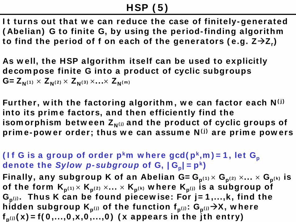
HSP (5)It turns out that we can reduce the case of finitely-generated (Abelian) G to finite G, by using the period-finding algorithm to find the period of f on each of the generators (e.g. Z Zr)
As well, the HSP algorithm itself can be used to explicitly decompose finite G into a product of cyclic subgroups G=ZN(1) × ZN(2) × ZN(3) ×...× ZN(m)
Further, with the factoring algorithm, we can factor each N(j)
into its prime factors, and then efficiently find the isomorphism between ZN(j) and the product of cyclic groups of prime-power order; thus we can assume N(j) are prime powers
(If G is a group of order pkm where gcd(pk,m)=1, let Gpdenote the Sylow p-subgroup of G, |Gp|=pk)Finally, any subgroup K of an Abelian G=Gp(1) × Gp(2) ×... × Gp(k) is of the form Kp(1) × Kp(2) ×... × Kp(k) where Kp(j) is a subgroup ofGp(j). Thus K can be found piecewise: For j=1,...,k, find the hidden subgroup Kp(j) of the function fp(j): Gp(j) X, wherefp(j)(x)=f(0,...,0,x,0,...,0) (x appears in the jth entry)

HSP (6)
If G is a group of order ptm where gcd(pt,m)=1, let Gp denote the Sylow p-subgroup of G, |Gp|=pt
Therefore, we can restrict attention to finite groups G=Gp
G=Gp ≈ Zpa1 × Zpa2 × Zpa3 ×...× Zpat
for some prime p and positive integers aj
Let a=max{aj}
We’ll explain the hidden subgroup algorithm by analogy to the period-finding algorithm, using eigenvalue-estimation analysis…
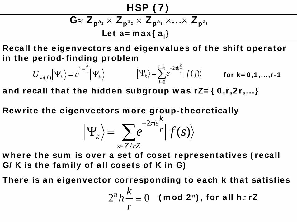
HSP (7)G≈ Zpa1 × Zpa2 × Zpa3 ×...× Zpat
Let a=max{aj}
Recall the eigenvectors and eigenvalues of the shift operator in the period-finding problem
krki
kfsh eU Ψ=Ψπ2
)( ∑−
=
−=Ψ
1
0
2)(
r
j
rkij
k jfeπ
for k=0,1,...,r-1
and recall that the hidden subgroup was rZ={0,r,2r,...}
Rewrite the eigenvectors more group-theoretically
∑∈
−=Ψ
rZZs
rkis
k sfe/
2)(
π
where the sum is over a set of coset representatives (recall G/K is the family of all cosets of K in G)
There is an eigenvector corresponding to each k that satisfies
02 ≡rkhn (mod 2n), for all h∈rZ
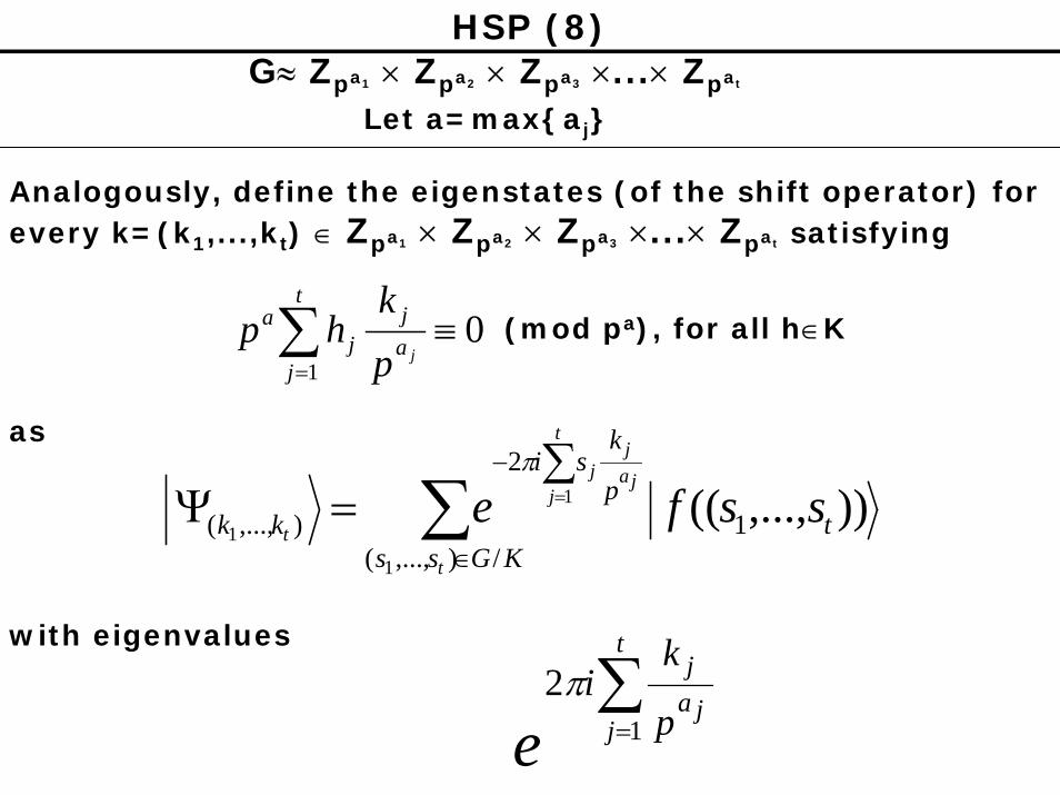
HSP (8)G≈ Zpa1 × Zpa2 × Zpa3 ×...× Zpat
Let a=max{aj}
Analogously, define the eigenstates (of the shift operator) for every k=(k1,...,kt) ∈ Zpa1 × Zpa2 × Zpa3 ×...× Zpat satisfying
01
≡∑=
t
jaj
ja
jpk
hp (mod pa), for all h∈K
as
∑∈
− ∑=Ψ =
KGsst
p
ksi
kkt
t
jja
jj
tssfe
/),...,(1
2
),...,(1
1
1)),...,((
π
with eigenvalues
∑=
t
jja
j
p
ki
e 1
2π

HSP (9)
The following algorithm determines a uniformly random k∈T, and by the above equation we can use enough random k to determine the subgroup K using linear algebra (like in Simon’s algorithm)
01
≡∑=
t
jaj
ja
jpk
hp (mod pa), for all h=(h1,…,ht)∈K
Let T be the set of all k=(k1,...,kt) that satisfy
HSP Algorithm:
1. Using QFT(paj) for j=1,...,t, and the black box for f, create the state
∑ ∑∑∑∈
−
=
−
=×××∈
Ψ⎟⎟
⎠
⎞
⎜⎜
⎝
⎛
⎟⎟
⎠
⎞
⎜⎜
⎝
⎛=
Tkk
p
xt
pkxip
x
pkxi
ZZZx
ta
t
tatta
a
tapapap
xexexfx1
0
21
01
21
1
111
21
)(ππ
LL
2. Apply QFT(pa1)-1⊗...⊗QFT(pat)-1⊗I to get
ktTk
kk Ψ∑∈
L1
3. Measure the control registers, output k1,...,kt

![Introduction to Quantum Information Processingjyard/qic710/Qic710Lec8-2017.pdf · Exercise: why are 2 bits ... Appendix A4.4 in [Nielsen & Chuang] ... with probability 𝛼2 2 * Showing](https://static.documents.pub/doc/80x56/5b51820c7f8b9ac4368c45eb/introduction-to-quantum-information-jyardqic710qic710lec8-2017pdf-exercise.jpg)

![Building a Quantum Information Processor using ... · [M. Nielsen and I. Chuang, Quantum Computation and Quantum Information (Cambridge, 2000)] • Quantum information processing](https://static.documents.pub/doc/80x56/5b8106597f8b9a2a088e3dd6/building-a-quantum-information-processor-using-m-nielsen-and-i-chuang.jpg)


![C:/Documents and Settings/valerio/My Documents/Physics ... · quantum information, the books of Nielsen and Chuang [3] or the short treatise by Le Bellac [4]. 1.1 Axioms, assumption](https://static.documents.pub/doc/80x56/5b68b2ce7f8b9af77c8cea55/cdocuments-and-settingsvaleriomy-documentsphysics-quantum-information.jpg)


