8186 RULES AND REGULATIONS Title 42— PUBLIC HEALTH

8186 RULES AND REGULATIONS

Title 42— PUBLIC HEALTHChapter IV— Environmental Protection

AgencyPART 410— NATIONAL PRIMARY AND

SECONDARY AMBIENT AIR QUALITY STANDARDSNotices of proposed rule-making pub-

lished in the F e d e r a l R e g is t e r on Jan-uary 30, 1971 (36 F.R. 1502) andMarch 26, 1971 (36 F.R. 5867) set forth regulations prescribing national primary and secondary ambient air quality standards proposed for adoption as Part 410 of 42 CFR. Interested persons were afforded an opportunity to participate in the ride-making by submitting com-ments. Following review of the proposed standards and consideration of the com-ments, the standards have been revised a s . described below and are being promulgated today.

National primary ambient air quality standards are those which, in the judg-ment of the Administrator, based on the air quality criteria and allowing an ade-quate margin of safety, are requisite to protect the public health.

National secondary ambient air quality standards are those which, in the judg-ment of the Administrator, based on the air quality criteria, are requisite to pro-tect the public welfare from any known or anticipated adverse effects associated with the presence of air pollutants in the ambient air.

The comments submitted to the En-vironmental Protection Agency reflect divergences of opinion among interested and informed persons as to the proper interpretation of available data on the public health and welfare effects of the six pollutants for which national am-bient air quality standards are being es-tablished. A number of comments ques-tion the feasibility of implementing the proposed standards. Because the Clean Air Act, as amended, does not permit any factors other than health to be taken into account in setting the primary standards, no revisions were made on this basis. In reviewing the proposed standards, the Environmental Protection Agency limited its consideration to com-ments concerning the validity of the scientific basis of the standards.

Current scientific knowledge of the health and welfare hazards of these air pollutants is imperfect. To increase and improve this knowledge, the Environ-mental Protection Agency will continue to conduct and support relevant re-search. At the same time, the need for increased knowledge of the health and welfare effects of air pollution cannot justify failure to take action based on knowledge presently available. The Clean Air Act, as amended, requires promulgation a t this time of national standards for six air pollutants on the basis of available data set forth in air quality criteria documents. Thus, the Administrator is required to make judg-ments as to the proper interpretation of presently available data and to establish national primary standards which in-

clude an adequate margin of safety to protect human health. Where the valid-ity of available research data has been questioned, but not wholly refuted, the Adm inistra to r has in each case promul-gated a national primary standard which includes a margin of safety adequate to protect the public health from adverse effects suggested by the available data.

The national primary standard for carbon monoxide, proposed bn January 30, 1971, was based on evidence that low levels of carboxyhemoglobin in human blood may be associated with impairment of ability to discriminate time intervals. This evidence is reflected in “Air Quality Criteria for Carbon Monoxide” (35 F.R. 4768). In the comments, serious questions were raised about the soundness of this evidence. Extensive consideration was given to this matter. The conclusions reached were that the evidence regarding impaired time-interval discrimination had not been refuted and that a less re-strictive national standard for carbon monoxide would therefore not provide the margin of safety which may be needed to protect the health of persons especially sensitive to the effects of ele-vated carboxyhemoglobin levels. The only change made in the national stand-ards for carbon monoxide was a modifi-cation of the 1-hour value. The revised standard affords protection from the same low levels of blood carboxyhemo-globin as a result of short-term expo-sure. The national standards for carbon monoxide, as set forth below, are in-tended to protect against the occurrence of carboxyhemoglobin levels above 2 per-cent. I t is the Administrator’s judgment that attainment of the national stand-ards for carbon monoxide will provide an adequate safety margin for protec-tion of public health and will protect against known and anticipated adverse effects on public welfare.

National standards for photochemical oxidants have also been revised. The re-vised national primary standard of 160 /tg./m* (0.08 p.pjm.) is based on evidence of increased frequency of asthma at-tacks in some asthmatic subjects on days when estimated hourly average concen-trations of photochemical oxidant reached 200 /ig./m.* (0.10 p.p.m.). A num-ber of comments raised serious questions about the validity of data used to sug-gest impairment of athletic performance a t lower oxidant concentrations. The revised primary standard includes a mar-gin of safety which is substantially be-low the most likely threshold level sug-gested by this data. It is the Administra-tor’s judgment that a primary standard of 160 /tg./m.* (0.08 p.pm.) as a 1-hour average will provide an adequate safety margin for protection of public health and will protect against known and an-ticipated adverse effects on public welfare.

National standards for hydrocarbons have been revised to make these stand-ards consistent with the above modifi-cations of the national standard for pho-tochemical oxidants. Hydrocarbons are a precursor of photochemical oxidants. The sole purpose of prescribing a hydro-

carbon standard is to control photochem-ical oxidants. Accordingly, Jh e above- described revisions of the national standards for photochemical oxidants necessitated a corresponding revision of the hydrocarbon standards.

National standards for nitrogen diox-ide have been revised to eliminate the proposed 24-hour average value. No ad-verse effects on public health or welfare have been associated with short-term exposure to nitrogen dioxide at levels which have been observed to occur in the ambient air. Attainment of the annual average will, in the Administrator’s judg-ment, provide an adequate safety mar-gin for protection of public health and will protect against known and antici-pated adverse effects on public welfare.

Appendices A through F, which de-scribe measurement methods, have been revised to clarify many technical points. As revised, each appendix describes a complete reference method for evaluat-ing the ambient concentration of a pol-lutant for which national ambient air quality standards are being established.

Nine months after the date of publi-cation of this notice, the States are re-quired to submit to the Administrator, in accordance with section 110 of the Act, implementation plans for the a t-tainment and maintenance of the na-tional primary and secondary standards specified in this part. Requirements for the preparation, adoption, and submittal of implementation plans were published by the Administrator, as proposed rule- making, in the F e d e r a l R e g is t e r on April 7, 1971 (36 F.R. 6680).

In consideration of the foregoing and in accordance with the statements in the notice of proposed rule-making, the na-tional primary and secondary ambient air quality standards, Part 410, are here-by promulgated effective upon publica-tion.

Dated: April 28, 1971.W il l ia m D. R u c k e l s h a u s ,

v Administrator.A new Part 410 is added to Chapter IV,

Title 42, Code of Federal Regulations as follows: sec.410.1 Definitions.410.2 Scope.410.3 Reference conditions.410.4 National primary am bient air quality

standards for sulfur oxides (sulfur dioxide).

410.5 National secondary ambient air qual-ity standards for sulfur oxides (sulfur dioxide).

410.6 National primary ambient-air qualitystandards for particulate matter.

41Q.7 National secondary am bient air qual-ity standards for particulate m atter.

410.8 National primary and secondary am-bient air quality standards for carbon monoxide.

410.9 National primary and secondary am-bient air quality standard for photochemical oxidants.

410.10 National primary and secondary am-bien t air quality standard for hydrocarbons.

410.11 National primary and secondary am-bient air quality standard for nitrogen dioxide.

FEDERAL REGISTER, VOL. 36, NO. 84— FRIDAY, APRIL 30, 1971

i

Appendix A—Reference Method for th e De-term ination of Sulfur Dioxide In th e Atmosphere ( Pararosanlline Method).

Appendix B—Reference Method for th e De-term ination of Suspended Particu-lates in th e Atmosphere (High Vol-ume Method).

Appendix C—Reference MetJjod for the Con-tinuous Measurement of Carbon monoxide in the Atmosphere (Non- dispersive Infrared Spectrometry).

Appendix D—Reference Method for th e Measurement of Photochemical Oxidants Corrected for Interfer-ences Due to Nitrogen Oxide and Sulfur Dioxide.

Appendix E—Reference Method for th e De-term ination of Hydrocarbons Cor-rected for Methane.

Appendix P—Reference Method for th e De-term ination of Nitrogen Dioxide (24-Hour Sampling Method).

Au t h o r i t y : The provisions of th is Part 410 issued under sec. 4, Public Law 91-604, Stat. 1679.§ 4 1 0 .1 D efin ition s.

(a) As used in this part, all terms not defined herein shall have the meaning given them by the Act.

(b) “Act” means the Clean Air Act, as amended (Public Law 91-604; 84 Stat. 1676).

(c) “Agency” means the Environ-mental Protection Agency.

(d) “Administrator” means the Ad-ministrator of the Environmental Pro-tection Agency.

(e) “Ambient air” means that portion of the atmosphere, external to buildings, to which thè general public has access.

(f) “Reference method” means a method of sampling and analyzing for an air pollutant, as described in an ap-pendix to this part.

(g) “Equivalent method” means any method of sampling and analyzing for an air pollutant which can be demon-strated to the Administrator’s satisfac-tion to have a consistent relationship to the reference method.§ 4 1 0 .2 Scope.

(a) National primary and secondary ambient air quality standards under sec-tion 109 of the Act are set forth in this part.

(b) National primary ambient air quality standards define levels of air quality which the Administrator judges are necessary, with an adequate margin of safety, to protect the public health. National secondary ambient air quality standards define levels of air quality which the Administrator judges neces-sary to protect the public welfare from any known or anticipated"adverse effects of a pollutant. Such standards are sub-ject to revision, and additional primary and secondary standards may be promul-gated as the Administrator deems neces-sary to protect the public health and welfare.

(c) The promulgation of national primary and secondary ambient air qual-ity standards shall not be considered in any manner to allow significant deterior-ation of existing air quality in any por-tion of any State.

RULES AND REGULATIONS

(d) The proposal, promulgation, or revision of national primary and second-ary ambient air quality standards shall not prohibit any State from establishing ambient air quality standards for that State or any portion thereof which are more stringent than the national standards.§ 4 1 0 .3 R eference conditions.

All measurements of air quality are corrected to a reference temperature of 25° C. and to a reference pressure of 760 millimeters of mercury (1,013.2 milli-bars).§ 4 1 0 .4 N ational prim ary am bient air

quality standards fo r su lfu r oxides (su lfu r d io x id e ) .

The national primary ambient air quality standards for sulfur oxides, measured as sulfur dioxide by the refer-ence method described in Appendix A to this part, or by an equivalent method, are:

(a) 80 micrograms per cubic meter (0.03 p.p.m.)—annual arithmetic mean.

(b) 365 micrograms per cubic meter (0.14 p.p.m.)—Maximum 24-hour con-centration not to be exceeded more than once per year.§ 4 1 0 .5 N ational secondary am bient air

quality standards fo r su lfu r ox ides (su lfu r d io x id e ) .

The national secondary ambient air quality standards for sulfur oxides, measured as sulfur dioxide by the refer-ence method described in Appendix A to this part, or by an equivalent method, are:

(a) 60 micrograms per cubic meter (0.02 p.p.m.)—annual arithmetic mean.

(b) 260 micrograms per cubic meter (0.1. p.p.m.)—maximum 24-hour con-centration not to be exceeded more than once per year, as a guide to be used in assessing implementation plans to achieve the annual standard.

(c) 1,300 micrograms per cuibc meter (0.5 p.p.m.)—maximum 3-hour concen-tration not to be exceeded more than once per year.§ 4 1 0 .6 N ational prim ary am bient air

quality standards fo r particu late m atter.

The national primary ambient air quality standards for particulate matter, measured by the reference method de-scribed in Appendix B to this part, or by an equivalent method, are:

(a) 75 micrograms per cubic meter— annual geometric mean.

(b) 260 micrograms per cubic meter— maximum 24-hour concentration not to be exceeded more than once per year.§ 4 1 0 .7 N ational secondary am bient air

quality standards fo r particu late m atter.

The national secondary ambient air quality standards for particulate matter, measured by the reference method de-scribed in Appendix B to this part, or by an equivalent method, are:

(a) 60 micrograms per cubic meter— annual geometric mean, as a guide to be used in assessing implementation plans to achieve the 24-hour standard.

SI 87

(b ) 150 micrograms per cubic meter— maximum 24-hour concentration not to be exceeded more than once per year.§ 4 1 0 .8 N ational prim ary and secondary

am bient air quality standards for car-b on m onoxide.

The national primary and secondary ambient air quality standards for carbon monoxide, measured by the reference method described in Appendix C to this part, or by an equivalent method, are:

(a) 10 milligrams per cubic meter (9 p.p.m.)—maximum 8-hour concentra-tion not to be exceeded more than once per year.

(b) 40 milligrams per cubic meter (35 p.p.m.)—maximum 1-hour concentra-tion not to be exceeded more than once per year.§ 4 1 0 .9 N ational prim ary and secondary

am bient air quality standards fo r photoch em ical oxidants.

The national primary and secondary ambient air quality standard for photo-chemical oxidants, measured and cor-rected for interferences due to nitrogen oxides and sulfur dioxide by the reference method described in Appendix D to this part, or by an equivalent method, is: 160 micrograms per cubic meter (0.08 p.p.m.)—maximum 1-hour concentra-tion not to be exceeded more than once per year. , f§ 4 1 0 .1 0 N ational prim ary and second-

ary am bient a ir quality standard for hydrocarbons.

The hydrocarbons standard is for use as a guide in devising implementation plans to achieve oxidant standards.

The national primary and secondary ambient air quality standard for hydro-carbons, measured and corrected for methane by the reference method de-scribed in Appendix E to this part, or by an equivalent method, is: 160 micrograms per cubic meter (0.24 p.p.m.)—m a xim um 3-hour concentration (6 to 9 a.m.) not to be exceeded more than once per year.§ 4 1 0 .1 1 N ational prim ary and second-

ary am bient air quality standard fo r nitrogen d ioxide.

The national primary and secondary ambient air quality standard for nitrogen dioxide, measured by the reference method described in Appendix F to this part, or by an equivalent method, is: 100 micrograms per cubic meter (0.05 p.p.m.)—annual arithmetic mean.Appe n d ix A.—Re f e r e n c e Me t h o d f o r t h e

De t e r m in a t io n o f Su l f u r Dio x id e i n t h e At m o s ph e r e (Pa r a r o s a n l l in e Me t h o d )

1. P r in c ip le a n d A p p lic a b i l i ty . 1.1 Sulfur • dioxide is absorbed from air in a solution of potassium tetrachloromercurate (TCM). A dichlorosulfltomercurate complex, which re-sists oxidation by the oxygen in the air, is formed (1, 2). Once formed, this complex is stable to strong oxidants (e.g., ozone, oxides of nitrogen). The complex is reacted with pararosaniline and formaldehyde to form in-tensely colored pararosaniline methyl sul-fonic acid (3). The absorbance of the solu-tion is measured spectrophotometrically.

1.2 The method is applicable to the meas-urement of sulfur dioxide in ambient air using sampling periods up to 24 hours.



2. R ange a n d S e n s itiv ity . 2.1 Concentra-tions of sulfur dioxide in the range of 25 to 1,050 „g/m.® (0.01 to 0.40 p.p.m.) can be meas-ured under th e conditions given. One can measure concentrations below 25 ^g./m.8 by sampling larger volumes of air, bu t only if the absorption efficiency of the particular sys-tem is first determined. Higher concentra-tions can be analyzed by using smaller gas samples, a larger collection volume, or a su it-able aliquot of the collected sample. Beer’s Law is followed through the working range from 0.03 to 1.0 absorbance units (0.8 to 27 /jg. of sulfite ion in 25 ml. final solution com-puted as SO2) .

2.2 The lower lim it of detection of sulfur dioxide in 10 ml. TCM is 0.75 ^g.j (based on twice the standard deviation) representing a concentration of 25 fig./roPSOa (0.01 p.p.m.) in an air sample of 30 liters.

3. In terferen ces. 3.1 The effects of the principal known interferences have been minimized or eliminated. Interferences by oxides of nitrogen are eliminated by sulfamic acid (4, 5), ozone by time-delay (8), and heavy metals by EDTA (ethylenediamine- tetroacetic acid, disodium salt) and phos-phoric acid (4, 6 ,). At least 60 fig. Fe (H I), 10 ng. M n(II), and 10 fig. C r(III) in 10 ml. absorbing reagent can be tolerated in the procedure. No significant interference was found w ith 10 ng. CU (II) and 22 fig. V(V).

4. Precision, A ccuracy, an d S ta b ility . 4.1 Relative standard deviation a t the 95 percent confidence level is 4.6 percent for the ana-lytical procedure using standard samples. (5)

4.2 After sample collection the solutions are relatively stable. At 22° C. losses of sulfur dioxide occur a t the rate of 1 percent per day. When samples are stored a t 5 ' C. for 30 days, no detectable losses of sulfur diox-ide occur. The presence of EDTA enhances th e stability of SO2 in solution, and the rate of decay is independent of the concentration of SO2. (7)

5. A ppara tu s.5.1 Sam plin g .5.1.1 A bsorber. Absorbers normally used

in air pollution sampling are acceptable for concentrations above 25 /tg./m.® (0.01 p.p.m .). An all-glass midget impinger, as shown in Figure Al, is recommended for 30-minute and 1-hour samples.

For 24-hour saimpling, assemble an ab-sorber from the following parts:

Polypropylene 2-port tube closures, special m anufacture (available from Bel-Art Prod-ucts, Pequannock, N .J.).

Glass impingers, 6 mm. tubing, 6 inches long, one end drawn to small diameter such th a t No. 79 jewelers will pass through, b u t No. 78 jewelers will not. (Other end fire polished.)

Polypropylene tubes, 164 by 32 mm. Nal- gene or equal).

5.1.2 P um p. Capable of maintaining an air pressure differential greater th an 0.7 a t-mosphere a t the desired flow rate.

5.1.3 Air F low m eter or C ritica l Orifice. A calibrated rotam eter or critical orifice ca-pable of measuring air flow within ± 2 per-cent. For 30-minute sampling, a 22-gauge hypodermic needle 1 inch long may be used as a critical orifice to give a flow of about 1 liter/m inute. For 1-hour sampling, a 23- gauge hypodermic needle five-eighths of an inch long may be used as a critical orifice to give a flow of about 0.5 liter/m inute. For 24 hour sampling, a 27-gauge hypodermic needle three-eighths of an inch long may be used to give a flow of about 0.2 liter/m inute. Use a membrane filter to protect the needle (Figure A la ).

6.2 A nalysis.5.2.1 S p ec tro p h o to m eter . Suitable for

measurement of absorbance a t 548 nm. w ith an effective spectral band width of less th a n 15 nm. Reagent blank problems may occur with spectrophotometers having greater

spectral band width. The wavelength cali-bration of th e instrum ent should be verified. If transm ittance is measured, th is can be converted to absorbance:

- A =log10 (1/T)6. R eagen ts.6.1 Sam pling.6.1.1 D istille d w ater. Must be free from

oxidants.6.1.2 A bsorbin g R eagen t [0.04 M P o ta s-

siu m T etrach lorom ercura te (TCM ) ]. Dissolve 10.86 g. mercuric chloride, 0.066 g. EDTA (thylenediaminetetraacetic acid, disodoum sa l t) , and 6.0 g. potassium chloride in water and bring to mark in a 1,000-ml. volumetric flask. (Caution: highly poisonous. If spilled on skin, flush off with water immediately). The pH of th is reagent should be approxi-mately 4.0, b u t it has been shown th a t there is no appreciable difference in collection efficiency over the range of pH 5 to pH 3.(7) The absorbing reagent is normally stable for 6 months. If a precipitate forms, discard the reagent.

5.2 A nalysis.6.2.L Su lfam ic A cid (0.6 p e rc e n t) . Dis-

solve 0.6 g. sulfamic acid in 100 ml. distilled water. Prepare fresh daily.

6.2.2 F orm aldeh yde (0.2 p e rc e n t) . Dilute 5 ml. formaldehyde solution (36-38 percent)' to 1,000 ml. w ith distilled water. Prepare daily.

6.2.3 S to ck Iod ine S o lu tion (0.1 N ) . Place 12.7 g. iodine in a 250-ml. beaker; add 40 g. potassium iodide and 25 ml. water. Stir until all is dissolved, then dilute to 1,000 ml. with distilled water.

6.2.4 Iod in e S o lu tio n (0.01 N ) . Prepare approximately 0.01 N iodine solution by di-lu ting 50 ml. of stock solution to. 500 ml. w ith distilled water.

6.2.5 S tarch In d ica to r S o lu tion . Triturate0.4 g. soluble starch and 0.002 g. mercuric iodide (preservative) with a little water, and add the paste slowly to 200 ml. boiling water. Continue boiling un til th e solution is clear; cool, and transfer to a glass-stoppered bottle.

6.2.6 S to ck S odiu m T h iosu lfa te S o lu tion (0.1 N ) . Prepare a stock solution by dissolving 25 g. sodium thiosulfate (Na2S20s,5H20) in1,000 ml. freshly boiled, cooled, distilled water and add 0.1 g. sodium carbonate to the solu-tion. Allow the solution to stand 1 day before standardizing. To standardize, accurately weigh, to the nearest 0.1 mg., 1.5 g. primary standard potassium iodate dried a t 180° C. and dilute to volume in a 500-ml. volumetric flask. To a 500-ml. iodine flask, pipet 50 ml. of iodate solution. Add 2 g. potassium iodide and 10 ml. of 1 N hydrochloric acid. Stopper th e flask. After 5 minutes, titra te w ith stock thiosulfate solution to a pale yellow. Add 5 ml. stanch indicator solution and continue the titra tion un til the blue color disappears. Calculate th e normality of th e stock solution:

WN = — X 2.80

MN=Normality of stock thiosulfate solu-

tion.M=Volume of thiosulfate required, nil.W =W eight of potassium iodate, grams.

103 (conversión of g. to mg.) X0.1 (fraction iodate used) 2 80 = 35.67 (equivalent weight of potassium iodate)

6.2.7 S od iu m T h iosu lfa te T itra n t (0.01 N ) . D ilute 100 ml. of the stock thiosulfate solu-tion to 1,000 ml. w ith freshly boiled distilled water.

Normality= Normality of stock solution X 0.100.

6.2.8 S ta n d a rd ize S u lfite S o lu tion for P repara tion o f W orking Su lfite-T C M Solu -tio n . Dissolve 0.3 g. sodium metabisulfite (Na2S2Os) or 0.40 g. sodium sulfite (Na2SOa) in 500 ml. of recently boiled, cooled, distilled water. (Sulfite solution is unstable; i t is therefore im portant to use water of the high-est purity to minimize th is instability.) This solution contains the equivalent of 320 to 400 zitg./ml. of SOa. The actual concentration of the solution is determined by adding excess iodine and back-titrating w ith standard sodium thiosulfate solution. To back-titrate, pipet 50 ml. of the 0.01 N iodine into each of two 500-ml. iodine flasks (A and B ). To flask A (blank) add 25 ml. distilled water; and to flask B (sample) pipet 25 ml. sulfite solution. Stopper th e flasks and allow to react for 5 minutes. Prepare the working sulfite-TCM Solution (6.2.9) a t the same tim e iodine solution is added to the flasks. By means of a buret containing standardized 0.01 N thio-sulfate, ti tra te each flask in tu rn to a pale yellow. Then add 5 ml. starch solution and continue the titra tion u n til the blue color disappears.

6.2.9 W orking Su tftte-T C M S olu tion . Pipet accurately 2 ml. of the standard solution into a 100 ml volumetric flask and bring to mark w ith 0.04 M TOM. Calculate the concentra-tion of sulfur dioxide in the working solu-tion:W 5Q./nü.= ( A- B) %> 35X0.02

A= Volume thiosulfate for blank, mLB=Volume thiosulfate for sample, ml.N =Norm ality of thiosulfate titran t.

32,000=M illiequivalent wt. of S 02, /tg.25= Volume standard sulfite solution,

ml.0.02=Dilution factor.

This solution is stable for 30 days if kept at 5 a C. (refrigerator). If not kept a t 5° C., prepare daily.

6.2.10 P urified P ararosaniline S tock Solu-t io n (0.2 p ercen t n o m in a l) .

6.2.10.1 D ye Specifica tions. The pararo-saniline dye m ust meet the following per-formance specifications: (1) th e dye must have a wavelength of maximum absorbance at 540 nm. when assayed in a buffered solu-tion of 0.1 M sodium acetate-acetic acid; (2) th e absorbance of the reagent blank, which is tem perature-sensitive (0.015 absorbance u n it /°C ), should not exceed 0.170 absorbance u n it a t 22° O. w ith a 1-cm. optical path length, when the blank is prepared accord-ing to th e prescribed analytical procedure and to the specified concentration of the dye;(3) th e calibration curve (Section 8.2.1) should have a slope of 0.030 ±0.002 absprb- ance units//ig. SO2 a t th is pa th length when th e dye is pure and the sulfite solution is properly standardized.

6.2.10.2 P repara tion o f S to ck S o lu tion . A specially purified (99-100 percent pure) so-lu tion of pararosaniline, which meets the above specifications, is commercially avail-able in the required 0.20 percent concen-tra tion (Harleco*). Alternatively, the dye may be purified, a stock solution prepared and then assayed according to th e proce-dure of Scaringelll, et al. (4)

6.2.11' P ararosaniline R eagen t. To a 250- ml. volumetric flask, add 20 ml. stock par-arosaniline solution. Add an additional 0.2 ml. stock solution for each percent the stock

•Hartmen-Leddon, 60th and Woodland Avenue, Philadelphia, PA 19143.


RULES AND REGULATIONS 8189assays below 100 percent. Then add 25 ml. 3 M phosphoric acid and dilute to volume w ith distilled water. This reagent Is stable for a t least 9 months.

7. P rocedure.7.1 S am plin g . Procedures are described

for short-term (30 m inutes and 1 hour) and for long-term (24 hours) sampling. One can select different combinations of sampling rate and tim e to meet special needs. Sample volumes should be adjusted, so th a t linearity is maintained between absorbance and con-centration over th e dynamic range.

7.1.1 30-M inu te an d 1-H our Sam plings. Insert a midget impinger into the sampling system, Figure Al. Add 10 ml. TCM solution to the impinger. Collect sample a t 1 lite r/ m inute for 30 minutes, or a t 0.5 liter/m inute for 1 hour, using either a rotameter, as shown J n Figure Al, or a critical orifice, as shown in Figure Ala, to control flow. Shield the absorbing reagent from direct sunlight during and after sampling by covering th e impinger with alum inum foil, to prevent deterioration. Determine the volume of air sampled by multiplying the flow rate by the tim e in m inutes and record the atmos-pheric pressure and tem perature. Remove and stopper the impinger. If the sample m ust be stored for more th an a day before analysis, keep it a t 5 s C. in a refrigerator (see 4.2).

7.1.2 24-H our Sam plin g . Place 50 ml. TCM solution in a large absorber and col-lect th e sample a t 0.2 liter/m inute for 24 hours from m idnight to midnight. Make sure no entrainm ent of solution results with the impinger. During collection and storage pro-tect from direct sunlight. Determine the total air volume by multiplying th e air flow rate by the tim e in minutes. The correction of 24-hour measurements for tem perature and pressure Is extremely difficult and is not ordinarily done. However, the accuracy of the measurement will be improved if mean-ingful corrections can be applied. If storage is necessary, refrigerate a t 5° C. (see 4.2).

7.2 A nalysis.7.2.1 Sam ple P repara tion . After collection,

if a precipitate is observed in the sample, remove it by centrifugation.

7.2.1.1 30-M inu te an d 1-H our Sam plep. Transfer the sample quantitatively to a 25- ml. volumetric flask; use about 5 ml. distilled water for rinsing. Delay analyses for 20 m in-utes to allow any ozone to decompose.

7.2.1.2 24-H our S am ple. Dilute the entire sample to 50 ml. with absorbing solution. Pipet 5 ml. of the sample into a 25-mL volumetric flask for chemical analyses. Bring volume to 10 ml. w ith absorbing reagent. Delay analyses for 20 m inutes to allow any ozone to decompose.

7.2.2 D eterm in a tio n . For each, set of de-term inations prepare a reagent blank by add-ing 10 ml. unexposed TCM solution to a 25- ml. volumetric flask. Prepare a control solu-tion by adding 2 ml. of working sulfite-TCM solution and 8 ml. TCM solution to a 25-ml. volumetric flask. To each flask containing ei-ther sample, control solution, „or reagent blank, add 1 ml. 0.6 percent sulfamic acid and allow to react 10 m inutes to de-stroy the n itrite from oxides of nitrogen. Accurately pipet in 2 ml. 0.2 percent formaldehyde solution, then 5 ml. pararosaniline solution. S tart a laboratory timer th a t has been set for 30 minutes. Bring all flasks to volume w ith freshly boiled and cooled distilled water and mix thoroughly. After 30 minutes and before 60 minutes, de-termine the absorbances of the sample (de-note as A ), reagent blank (denote as Ao) and the control solution a t 548 nm. using 1-cm. optical path length cells. Use distilled water, no t the reagent blank, as the reference. (No t e ! This is im portant because of the color sensitivity of the reagent blank to tem pera-ture changes which can be induced in the

cell compartm ent of a spectrophotometer.) Do not allow the colored solution to stand in the absorbance cells, because a film of dye may be deposited. Clean cells w ith alcohol after use. If the tem perature of the determi-nations does not differ by more th an 2° C. from the calibration tem perature (8.2), the reagent blank should be w ithin 0.03 absorb-ance un it of the y-intercept of the calibra-tion curve (8.2). If the reagent blank differs by more than 0.03 absorbance u n it from th a t found in the calibration curve, prepare a new curve.

7.2.3 A bsorbance R ange. If the absorbance of the sample solution ranges between 1.0 and 2.0, the sample can be diluted 1:1 with a portion of the reagent blank and read within a few minutes. Solutions with higher absorbance can be diluted up to sixfold with th e reagent blank in order to obtain onscale readings w ithin 10 percent of the true ab-sorbance value.

8. C alibra tion an d Efficiencies.8.1 F low m eters a n d H ypoderm ic N eedle.

Calibrate flowmeters and hypodermic nee-dle (8) against a calibrated wet test meter.

8.2 C alibra tion C urves.8.2.1 P rocedure w ith S u lfite S o lu tion . Ac-

curately pipet graduated am ounts of the working sulflte-TCM solution (6.2.9) (such as 0, 0.5, 1, 2, 3, and 4 ml.) into a series of 25-ml. volumetric flasks. Add sufficient TCM solution to each flask to bring the volume to approximately 10 ml. Then add the re m a in in g reagents as described in 7.2.2. For maximum precision use a constant-tem perature bath. The tem perature of calibration m ust be m aintained w ithin ±1° C. and in the range of 20° to 30° C. The tem perature of calibra-tion and the tem perature of analysis m ust be w ithin 2 degrees. Plot the absorbance against the to tal concentration in /tg. SOa for the corresponding solution. The total tig. SOa in solution equals the concentration of the standard (Section 6.2.9) in /tg. SOa/ml. times the ml. sulfite solution added (tig. SOa= /ig ./m l. SOa xm l. added). A linear relation-ship should be obtained, and the y-intercept should be. w ithin 0.03 absorbance u n it of the zero standard absorbance. For maximum pre-cision determine the line of best fit using regression analysis by the method of least squares. Determine th e slope of the line of best fit, calculate its reciprocal and denote as Ba. Bs is the calibration factor. (See Sec-tion 6.2.10.1 for specifications on the slope of the calibration curve). This calibration fac-to r can be used for calculating results pro-vided there are no radical changes in tem perature or pH. At least one control sample containing a known concentration of SO2 for each series of determinations, is recommended to insure the reliability of th is factor.

8.2.2 Procedure w ith SOa P erm ea tion Tubes.

8.2.2.1 G eneral C onsiderations. Atmos-pheres containing accurately known amounts of sulfur dioxide at levels of interest can be prepared using permeation tubes. In the systems for generating these atmospheres, the permeation tube emits S02 gas at a known, low, constant rate, provided the tem -perature of the tube is held constant (±0.1° C.) and provided the tube has been accu-rately calibrated a t th e tem perature of use. The S02 gas permeating from the tube is carried by a low flow of inert gas to a mix-ing chamber where it is accurately diluted with S02-free air to the level of interest and th e sample taken. These systems are shown schematically in Figures A2 and A3 and have been described in detail by O’Keeffe and Ortman (9 ) , Scaringelli, Frey, and Saltzman (1 0 ), and Scaringelli, O’Keeffe, Rosenberg, and Bell (1 1 ).

8.2.2.2 P repara tion o f S ta n d a rd A tm o s-pheres. Permeation tubes may be prepared

or purchased. Scaringelli, O’Keeffe, Rosen-berg, and Bell ( II) give detailed, explicit directions for permeation tube calibration. Tubes w ith a certified permeation ra te are available from the National Bureau of Stand-ards. Tube permeation rates from 0.2 to 0.4 /ig./m inute inert gas flows of about 50 m l./ m inute and dilution air flow rates from 1.1 to 15 liters/m inutes conveniently give stand-ard atmospheres containing desired levels of S 02 (25 to 390 /tg./m.3; 0.01 to 0.15 p.p.m. S 02) . The concentration of S02 in any stand-ard atmosphere can be calculated as follows:

P X 10 8 C = --------

Where:O = Concentration of SO2, n g ./m ? a t ref-

erence conditions.P =T ube permeation rate,/tg./m inute. Rd=Flow rate of dilution air, liter/m inute

a t reference conditions.R i=Flow rate of inert gas, liter/m inute a t

reference conditions.8.2.2.3 S am p lin g a n d P repara tion o f C ali-

b ra tio n C urve. Prepare a series (usually six) of standard atmospheres containing SOa levels from 25 to 390 /tg. S02/m .8. Sample each atmosphere using similar apparatus and tak -ing exactly the same air volume as will be done in atmospheric sampling. Determine absorbances as directed in 7.2. Plot the con-centration of SO2 in /ig./m.3 (x-axis) against A—A0 values (y-axis), draw the straight line of best fit and determine the slope. Alter-natively, regression analysis by the method of least squares may be used to calculate the slope. Calculate th e reciprocal of the slope and denote as Bg.

8.3 S am plin g E fficiency. Collection effi-ciency is above 98 percent; efficiency may fall off, however, a t concentrations below 25 /ig./m.3. (1 2 ,1 3 )

9. C alcu la tions.9.1 C onversion o f V olum e. Convert the

volume of air sampled to the volume a t ref-erence conditions of 25° C. and 760 mm. Hg. (On 24-hour samples, th is may not be possible.)

P 298Vb =V X---- X---------

760 t+273Va—Volume of air a t 25° C. and 760 mm.

Hg, liters.V = Volume of air sampled, liters.P =Barom etric pressure, mm. Hg. t = Temperature of air sample, °C.9.2 S u lfu r D ioxide C on cen tra tion .9.2.1 When sulfite solutions are used to :

prepare calibration curves, compute the con- 1 centration of sulfur dioxide in the sam ple: /

(A-Ao) (10«) (B.)/ig. S02/m .3= ----------------------------xD

Vr

A = Sample absorbance.A0=R eagent blank absorbance.103—Conversion of liters to cubic meters.Vb = T he sample corrected to 25® C. and

760 mm. Hg, liters,Bs i= Calibration factor, /tg./absorbance

unit.D = Dilution factor.

For 30-minute and 1-hour samples, D = l.

For 24-hour samples, D = 10.9.2.2 When S02 gas standard atmospheres

are used to prepare calibration curves, com-pute the. sulfur dioxide in the sample by the following formula:

S 02, /ig./m.3 = (A - Ao) X BgA = Sample absorbance.Ao=Reagent blank absorbance.Bg= (See 8.2.2.3).9.2.3 C onversion o f ng./m .* to p .p .m .= U

desired, the concentration of su lfur dioxide



may be calculated as p.p.m. SO2 a t reference conditions as follows:

p.p.m. S02=/ig. S02/m .8 X3.82 X10-*10. R eferences.

(1) West, P. W., and Gaeke, G. O., “Fixa- / * tion of Sulfur Dioxide as Sulfitomer-

curate III and Subsequent Colori-m etric Determ ination”, A nal. C hem . 28, 1816 (1956).

(2) Epbraims, F., “Inorganic Chemistry,”p. 562, Edited by P.C.L. Thorne and E. R. Roberts, 5th Edition, In ter-science. (1948).

(3) Lyles, G. R., Dowling, F. B., and Blanch-ard, V. J., “Q uantitative determ ina-tion of Formaldehyde in Parts Per Hundred Million Concentration Lev-el”, J. A ir Poll. C on t. Assoc. 15, 106 (1965).

(4) Scaringelli, F. P., Saltzman, B. E., andFrey, S. A., “Spectrophotometric De-term ination of Atmospheric Sulfur Dioxide”, A nal. C hem . 39,1709 (1967).

(5) Pate, J . B., Ammons, B. E., Swanson,G. A., Lodge, J . P., Jr., “N itrite In -terference in Spectrophotometric De-term ination of Atmospheric Sulfur Dioxide”, A nal. C hem . 37,942 (1965).

(6) Zurlo, N. and Grifflni, A. M„ “Measure-m ent of th e S02 Content of Air in the Presence of Oxides of Nitrogen and Heavy Metals”, M ed. Lavoro, 53, 330 (1962).

(7) Scaringelli, F. P., Elfers, L., Norris, D.,and Hochheiser, S., “Enhanced Sta-bility of Sulfur Dioxide in Solution”, A nal. C hem . 42, 1818 (1970).

(8) Lodge, J. P. Jr., Pate, J. B., Ammons,B. E. and Swanson, G, A., “Use of Hypodermic Needles as Critical Ori-fices in Air Sampling,” J . A ir Poll. C ont. Assoc. 16, 197 (1966).

(9) O’Keeffe, A. E„ and Ortman, G. C.,“Primary Standards for Trace Gas Analysis”, Anal. C hem . 38, 760 (1966).

(10) Scaringelli, F. P., Frey, S. A., and Saltz-man, B. E., “Evaluation of Teflon Permeation Tubes for Use with Sulfur Dioxide”, A m er. In d . H ygiene Assoc. J. 28, 260 (1967).

(11) Scaringelli, F. P., O’Keeffe, A. E., Rosen-berg, E., and Bell, J . P., “Preparation of Known Concentrations of Gases and Vapors with Permeation Devices Calibrated Gravimetrically”, A nal. C hem . 42,871 (1970).

(12) Urone, P., Evans, J. B., and Noyes, C. M.,‘ “Tracer Techniques in Sulfur Di-oxide Colorimetric and Conductio- metric Methods”, A nal C hem . 37,1104 (1965).

(13) Bostrom, C. E.,'“The Absorption of Sul-fu r Dioxide a t Low Concentrations (p.p.m.) Studied by an Isotopic Tracer Method”, In te rn . J. A ir W ater Poll. 9, 33 (1965).

HYPODERMICNEEDLE

TO AIR PUMP

IMPINGER

Figure A1. Sampling train.


RULES AND REGULATIONS 8191

CYLINDER AIR OR

NITROGEN

Figure A2. Apparatus for gravimetric calibration and field use.

Appe n d ix B—Re f e r e n c e Me t h o d f o b t h e De t e r m in a t io n o f Su s pe n d e d Pa r t ic u l a t e s i n t h e At m o s ph e r e (Hig h Vo l u m e Me t h o d )1. P rin cip le and A p p lica b ility .1.1 Air Is drawn into a covered housing

and through a filter by means of a high-flow-rate blower a t a flow rate (1.13 to 1.70 m.3/ min.; 40 to 60 ft.3/m in.) th a t allows sus-pended particles having diameters of less th an 100 nm.. (Stokes equivalent diameter) to pass to the filter surface. (1 ) Particles w ithin the size range of 100 to 0.1/un. diame-ter are ordinarily collected on glass fiber fil-ters. The mass concentration of suspended particulates in the ambient air (tig ./m .*) is computed by measuring th e mass of collected particulates and the volume of air sampled.

1.2 This method is applicable to measure-m ent of the mass concentration of suspended particulates in ambient air. The size of the sample collected is usually adequate for other analyses.

2. R ange a n d S e n s itiv ity .2.1 When the sampler is operated a t an

average flow rate of 1.70 m.3/m in. (60 ft.3/ min.) for 24 horns, an adequate sample will be obtained even in an atmosphere having concentrations of suspended particulates as low as 1 Ag./m.3. If particulate levels are unusually high, a satisfactory sample may be obtained in 6 to 8 hours or less. For deter-mination of average concentrations of sus-pended particulates in ambient air, a stand-ard sampling period of 24 hours is recommended.

2.2 Weights are determined to th e near-est milligram, airflow rates are determined to the nearest 0.03 m.*/min. (1.0 ft.3/m in .), times are determined to the nearest 2 minutes, and mass concentrations are re-ported to the nearest microgram per cubic meter.'

3. In terferen ces.3.1 Particulate m atter th a t Is oily, such

as photochemical smog or wood smoke, may block the filter and cause a rapid drop in airflow a t a nonuniform rate. Dense fog or high hum idity can cause the filter to become too wet and severely reduce th e airflow through the filter.

3.2 Glass-fiber filters are comparatively Insensitive to changes in relative numidlty, b u t collected particulates can be hygro-scopic. (2)

4. P recision, A ccuracy, a n d S ta b ility .4.1 Based upon collaborative testing, the

relative standard deviation (coefficient of variation) for single analyst variation (re-peatability of th-> method) is 3.0 percent. The corresponding value for m ultilaboratory variation (reproducibility of the method) is 3.7 percent. (3)

4.2 The accuracy w ith which th e sampler measures the true average concentration depends upon th e constancy of the airflow ra te through th e sampler. The airflow rate is affected by the concentration and th e nature of the dust in the atmosphere. Under these conditions th e error in the measured aver-age concentration may be in excess of ±50 percent of the tru e average concentration, de-pending on th e ‘am ount of reduction of air-flow rate and on the variation of the mass concentration of dust with tim e during the 24-hour sampling period. (4)

5. A ppara tu s.5.1 Sam plin g .5.1.1 Sam pler. The sampler consists of

three un its; (1) the faceplate and gasket, (2) th e filter adapter assembly, and (3) the m otor un it. Figure B1 shows an exploded view of these parts, their relationship to each other, and how they are assembled. The sampler m ust be capable of passing environ-m ental air through a 406.5 cm.3 (63 in.3) portion of a clean 20.3 by 25.4 cm. (8- by 10-ln.) glass-fiber filter a t a rate of a t least 1.70 m.Vinin. (60 ft.3/m in .). The motor m ust be capable of continuous operation for 24- hour periods w ith inpu t voltages ranging from 110 to 120 volts, 50-60 cycles a lternat-ing current and m ust have third-w ire safety ground. The housing for th e motor un it may be of any convenient construction so long as the un it remains airtigh t and leak- free. The life of the sampler m otor can be extended by lowering the voltage by about 10 percent w ith a small “buck or boost” transform er between the sampler and power outlet.

5.1.2 S am pler S h e lter . I t is im portant th a t the sampler be properly installed in a suitable shelter. The shelter is subjected to extremes of tem perature, humidity, and all types of air pollutants. For these reasons th e materials of the shelter m ust be chosen carefully. Properly painted exterior plywood or heavy gauge alum inum serve well. The sampler m ust be mounted vertically in the shelter so th a t the glass-fiber filter is paral-lel with the ground.. The shelter m ust be provided w ith a roof so th a t the filter is pro-tected from precipitation and debris. The internal arrangement and configuration of a suitable shelter w ith a gable roof are shown in Figure B2. The clearance area between the main housing and the roof a t its closest point should be 580.5± 193.5 cm.3 (90±30 in.3) . The main housing should be rectangu-lar, w ith dimensions of about 29 by 36 cm. (11% by 14 in .).

5.1.3 R o ta m e ter . Marked In arbitrary units, frequently 0 to 70, and capable of being calibrated. O ther devices of a t least comparable accuracy may be used.



5.1.4 Orifice C a lib ra tion U n it. Consisting of a m etal tube 7.6 cm. (3 in.) ID and 15.9 cm. (6)4 in.) long w ith a static pressure tap5.1 cm. (2 in.) from one end. See Figure B3. The tube end nearest th e pressure tap is flanged to about 10.8 cm. (4)4 in.) OD w ith a male thread of the same size as the inlet end of the high-volume air sampler. A single metal plate 9.2 cm. (3% in.) in diam eter and0.24 cm. (%2 in.) th ick w ith a central orifice 2.9 cm. (1)4 in.) in diam eter is held in place a t the air inlet end w ith a female threaded ring. The other end of th e tube is flanged to hold a loose female threaded coupling, which screws onto the in let of the sampler. An 18- hole m etal plate, an integral part of the unit, is positioned between the orifice and sampler to sim ulate the resistance of a clean glass- fiber filter. An orifice calibration u n it is shown in Figure B3.

5.1.5 D ifferen tia l M an om eter. Capable of measuring to a t least 40 cm. (16 in.) of water.

5.1.6 P o sitive D isp la cem en t M eter. Cali-brated in cubic meters or cubic feet, to be used as a primary standard.

5.1.7 B arom eter. Capable of measuring a t-mospheric pressure to the nearest mm.

5.2 A nalysis.5.2.1 F ilte r C on d itio n in g E n viron m en t.

Balance room or desiccator m aintained a t 15° to 35 °C. and less th an 50 percent relative humidity.

5.2.2 A n a ly tica l B alance. Equipped w ith a weighing chamber designed to handle u n -folded 20.3 by 25.4 cm. (8- by 10-in.) filters and having a sensitivity of 0.1 mg.

5.2.3 L ig h t Source. Frequently a table of th e type used to view X-ray films.

5.2.4 N u m berin g D evice. Capable of p rin t-ing identification numbers on the filters.

6. R eagen ts.6.1 F ilter M edia. Glass-fiber filters having

a collection efficiency of a t least 99 percent for particles of 0.3 /¿m. diameter, as measured by th e DOP test, are suitable for th e quanti-tative measurement of concentrations of sus-pended particulates, (5) although some other medium, such as paper, may be desirable for some analyses. If a more detailed analysis is contemplated, care m ust be exercised to use filters th a t contain low background concen-trations of th e pollu tant being investigated. Careful quality control is required to deter-mine background values of these pollutants.

7. Procedure.7.1 Sam plin g .7.1.1 F ilter P repara tion . Expose each filter

to th e light source and inspect for pinholes, particles, or other imperfections. Filters w ith visible imperfections should riot be used. A small brush is useful for removing particles. Equilibrate th e filters in th e filter condition-ing environment for 24 hours. Weigh -the filters to th e nearest milligram; record tare weight and filter identification number. Do no t bend or fold the filter before collection of th e sample.

7.1.2 Sam ple C ollection . Open the shelter, loosen th e wing nuts, and remove th e face-plate from the filter holder. Install a num -bered, preweighed, glass-fiber filter in posi-tion (rough side up ), replace th e faceplate w ithout disturbing th e filter, and fasten securely. Undertightening will allow air leak-age, overtightening will damage th e sponge- rubber faceplate gasket. A very light applica-tion of talcum powder may be used on the sponge-rubber faceplate gasket to prevent th e filter from sticking. During inclement weather th e sampler may be removed to a protected area for filter change. Close the roof of the shelter, run the sampler for about 5 minutes, connect the rotameter to the nipple on th e back of th e sampler, and read the rotam eter ball w ith rotameter in a verti-cal position. Estimate to the nearest whole number. If th e ball is fluctuating rapidly, tip the rotam eter and slowly straighten it

u n til the ball gives a constant reading. Dis-connect the rotam eter from th e nipple; re-cord th e in itial rotam eter reading and the starting tim e and date on th e filter folder. (The rotam eter should never be connected to the sampler except when the flow is being measured.) Sample for 24 hours from mid-nigh t to midnight and take a final rotam eter reading. Record th e final rotam eter reading and ending time and date on the filter folder. Remove the faceplate as described above and carefully remove th e filter from th e holder, touching only the outer edges. Fold th e filter lengthwise so th a t only surfaces w ith col-lected particulates are in contact, and place in a m anila folder. Record on the folder th e filter number, location, and any other factors, such as meteorological conditions or razing of nearby buildings, th a t m ig h t affect the results. If the sample is defective, void it a t th is time. In order to obtain a valid sample, th e high-volume sampler m ust be operated w ith th e same rotam eter and tubing th a t were used during its calibration.

7.2 A nalysis. Equilibrate the exposed fil-ters for- 24 hours in th e filter conditioning environment, th en reweigh. After they are weighed, th e filters may be saved for detailed chemical analysis.

7.3 M aintenance.7.3.1 S am pler M otor. Replace brushes

before they are worn to the point where motor damage can occur.

7.3.2 F acepla te G asket. Replace when th e margins of samples are no longer sharp. The gasket may be sealed to the faceplate w ith rubber cement or double-sided adhesive tape.

7.3.3 R o ta m eter . Clean as required, using alcohol.

8. C alibra tion .8.1 P urpose. Since only a small portion

of the to tal air sampled passes through the rotam eter during measurement, the rotam -eter m ust be calibrated against actual air-flow w ith th e orifice calibration unit. Before the orifice calibration u n it can be used to calibrate the rotameter, th e orifice calibra-tion u n it itself m ust be calibrated against the positive displacement primary standard.

8.1.1 Orifice C a lib ra tion U n it. Attach the orifice calibration u n it to th e intake end of the positive displacement primary stand-ard and attach a high-volume motor blower u n it to th e exhaust end of the primary standard. Connect one end of a differential manometer to the differential pressure tap of th e orifice calibration u n it and leave the other end open to th e atmosphere. Operate the high-volume motor blower u n it so th a t a series of different, b u t constant, airflows (usually six) are obtained for definite tim e periods. Record the reading on the differen-tia l manometer a t each airflow. The different constant airflows are obtained by placing a series of loadplates, one a t a time, between the calibration u n it and the primary stand-ard. Placing th e orifice before the in let re-duces the pressure a t the inlet of the primary standard below atmospheric; therefore, a correction m ust be made for the increase in volume caused by th is decreased in let pres-sure. A ttach one end of a second differential m anam eter to an in let pressure tap of th e primary standard and leave the other open to the atmosphere. During each of the con-stan t airflow measurements made above, measure the true inlet pressure of th e primary standard w ith th is second differen-tia l manometer. Measure atmospheric pres-sure and tem perature. Correct th e measured air volume to true air volume as directed in 9.1.1, then obtain true airflow rate, Q, as directed in 9.1.3. Plot the differential manom-eter readings of the orifice u n it versus Q.

8.1.2 H igh -V olu m e Sam pler. Assemble a high-volume sampler w ith a clean filter in place and rim for a t least 5 minutes. A ttach a rotameter, read the ball, adjust so th a t the ball reads 65, and seal the adjusting mech-

anism. so th a t i t oannot be changed easily. S hut off motor, remove the filter, and attach the orifice calibration u n it in its place. Op-erate th e high-volume sampler a t a series of different, b u t constant, airflows (usually six). Record th e reading of the differential ma-nometer on the orifice calibration un it, and record the readings of th e rotam eter a t each flow. Measure atmospheric pressure and tem -perature. Convert th e differential manometer reading to m.s/m in., Q, then plot rotameter reading versus Q.

8.1.3 C orrection fo r D ifferences in P ressure or T em pera ture . See Addendum B.

9. C alcu la tions.9.1 C alibra tion of Orifice.9.1.1 True A ir V olum e. Calculate th e air

volume measured by th e positive displace-m ent primary standard.

(P.-Pm)Va = -------------(Vm)

PaVa= True air volume a t atmospheric pres-

sure, m.* *Pa= Barometric pressure, mm. Hg.Pm= Pressure drop a t inlet of primary

standard, mm. Hg.Vm=V olume measured by primary stand-

ard, m*9.1.2 C onversion F actors.Inches Hg. x 25.4=mm. Hg.Inches water x 73.48 x 10-*=inches Hg.Cubic feet air x 0.0284=cubic meters air.9.1.3 True A irflow R a te .

V.Q = —

TQ = Flow rate, m.*/min.T =T im e of flow, min.9.2 S am ple V olum e.9.2.1 V olum e C onversion. Convert the ini-

tia l and final rotam eter readings to true airflow rate, Q, using calibration curve of 8.1.2.

9.2.2 C alcu la te vo lu m e o f air sa m p ledQiQr

V = ------- XT2

V =Air volume sampled, m.*Q i= In itia l airflow rate, m.*/min.Q t= Final airflow rate, m.8/m in .T=Sam pling time, min.

9.3 C alcu la te m ass co n cen tra tio n o f sus-p en d ed p a rticu la te s

(W i-W i) xio«S.P.=-------------- —

VS.P.=Mass concentration of suspended

particulates, /xg/m.*Wi = In itial weight of filter, g.W t= Final weight of filter, g.

V= Air volume sampled, m.*10«=Conversion of g. to ¡1%.

10. R eferences.(1) Robson, C. D., and Foster, K. E ,

“Evaluation of Air Particulate Sam-pling Equipm ent”, Am. In d . Hyg. Assoc. J . 24, 404 (1962).

(2) Tierney, G. P.,. and Conner, W. D.,“Hygroscopic Effects on Weight Deter-m inations of Particulates Collected on Glass-Fiber Filters”, A m . In d . Hyg. Assoc. J. 28, 363 (1967).

(3) Unpublished data based on a collabora-tive tes t involving 12 participants, conducted under the direction of the Methods Standardization Services Sec-tion of the National Air Pollution Con-trol Administration, October, 1970.

(4) Harrison, W. K., Nader, J . S., and Fug-man, F. S., “Constant Flow Regulators for High-Volume Air Sampler”, Am . In d . Hyg. Assoc. J . 21, 114-120 (1960).


RULES AND REGULATIONS 8193(5) Pate, J. B., and Tabor, E. C., “Analytical

Aspects of the Use of Glass-Fiber Fil-ters for the Collection and Analysis of Atmospheric Particulate M atter”, A m . In d . H yg. Assoc. J . 23, 144-150 (1962).

Ad d e n d a uA. A lte rn a tiv e E q u ip m en t.A modification of the high-volume sampler

incorporating a method for recording the actual airflow over the entire sampling pe-riod has been described, and is acceptable for measuring th e concentration of sus-pended particulates (Henderson, J. S., Eighth Conference on Methods in Air Pollution and Industrial Hygiene Studies, 1967, Oakland, Calif.). This modification consists of an ex-haust orifice meter assembly connected through a transducer to a system for con-tinuously recording airflow on a circular chart. The volume of air sampled is cal-culated by the following equation:

V =Q X T.Q=Average sampling rate, m.s/m in.T=Sam pling time, minutes.

The average sampling rate, Q, is determined from the recorder chart by estim ation if the flow rate does not vary more th an 0.11 m.®/ min. (4 ft.s/m in.) during the sampling pe-riod. If the flow rate does vary more than 0:11 m.® (4 ft.s/m in.) during the sampling period, read the flow rate from the chart a t 2-hour intervals and take the average.

B. P ressure and T em pera tu re C orrections.

If the pressure or tem perature during high-volume sampler calibration is substan-tially different from the pressure or tempera-ture during orifice calibration, a correction of the flow rate, Q, may be required. If the pressures differ by no more th an 15 percent and the tem peratures differ by no more than 100 percent (°C ), the error in the u n -corrected flow rate will be no more th an 15 percent. If necessary, obtain the corrected flow rate as directed below. This correction applies only to orifice meters having a con-stan t orifice coefficient. The coefficient for the calibrating orifice described in 5.1.4 has been shown experimentally to be constant over the normal operating range of the high- volume sampler (0.6 to 2.2 m.»/min.; 20 to 78 ft .y m ln .) . Calculate corrected flow rate:

Qa=Corrected flow rate, m.3/m in . *Qi=Flow rate during high-volume sampler

calibration (Section 8.1.2), m.®/min.Tx=Absolute tem perature during orifice

u n it calibration (Section .8.1.1), °K or 'B .

Pi=Barom etric pressure during orifice un it calibration (Section 8.1.1), mm. Hg.

Ta=Absolute tem perature during high- volume sampler calibration (Section8.1.2) , °K or "B.

Pa= Barometric pressure during high-vol-ume sampler calibration (Section8.1.2) , wmi- Hg.

No. 84—Pt. n -----2 FEDERAL REGISTER, VOL. 36, NO. 84— FRIDAY, APRIL 30, 1971

8194 RULES ANO REGULATIONS

Figure B2. Assembled sampler and shelter.

Figure B3.

Appe n d ix C—Re f e r e n c e Me t h o d f o b t h e Co n t in u o u s Me a s u r e m e n t o f Ca r b o n Mo n o x id e i n t h e At m o s ph e r e (No n - Dis pe r s iv e I n f r a r e d Spe c t r o m e t r y )

1. P rincip le ancL A p p lica b ility .1.1 This method is based on the absorp-

tion of infrared radiation by carbon mon-oxide. Energy from a source emitting radia-tion in the infrared region is split into parallel beams and directed through ref-erence and sample cells. Both beams pass into matched cells, each containing a selec-

Orifice calibration unit.

tive detector and CO. The CO in the cells absorb infrared radiation only a t its charac-teristic frequencies and the detector is sensi-tive to those frequencies. W ith a nonabsorb-ing gas in the reference cell, and w ith no CO in the sample cell, the signals from both detectors are balanced electronically. Any CO introduced into the sample cell will absorb radiation, which reduces th e tem per-ature and pressure in the detector cell and displaces a diaphram. This displacement is detected electronically and amplified to pro-vide an output signal.

1.2 This method is applicable to th e de-term ination of carbon monoxide in ambient air, and to the analysis of gases under pressure.

2. R ange an d S e n s itiv ity .2.1 Instrum ents are available th a t meas-

ure in th e range of 0 to 58 mg./m.3 (0-50 p.p.m.), which is the range most commonly used for urban atmospheric sampling. Most instrum ents measure in additional ranges.

2.2 Sensitivity is 1 percent of full-scale response per 0.6 mg. CO/m.* (0.5 p.p.m .).

3. In terferences.3.1 Interferences vary between individual

instrum ents. The effect of carbon dioxide interference a t normal concentrations is minim al. The primary interference is water vapor, and with no correction may give an Interference equivalent to as high as 12 mg. CO/m.® Water vapor interference can be minimized by (a) passing the air sample through silica gel or similar drying agents, (b) m aintaining constant hum idity in the sample and calibration gases by refrigera-tion, (c) saturating th e air sample and cali-bration gases to m aintain constant hum id-ity or (d) using narrowband optical filters in combination with some of these measures.

3.2 Hydrocarbons a t am bient levels do not ordinarily interfere.

4. P recision, A ccuracy, a n d S ta b ility ., 4.1 Precision determined w ith calibration

gases is ±0.5 percent full scale in th e 0-58 mg./m.3 range.

4.2 Accuracy depends on Instrum ent linearity and the absolute concentrations of the calibration gases. An accuracy of ±1 percent of full scale in the 0-58 mg./m.* range can be obtained.

4.3 Variations in am bient room tem pera-tu re can cause changes equivalent to as m uch as 0.5 mg. CO/m.* per °C. This effect can be minimized by operating th e analyzer in a tem perature-controlled room. Pressure changes between span checks, will cause changes in instrum ent response. Zero drift is usually less th an ± 1 percent of full scale per 24 hours, if cell tem perature and pres-sure are m aintained constant.

5. A ppara tu s.5.1 Carbon M onoxide A nalyzer. Commer-

cially available instrum ents should be in -stalled on location and demonstrated, pref-erably by th e m anufacturer, to meet or exceed m anufacturers specifications' and those described in th is method.

5.2 Sam ple In tro d u c tio n S ystem . Pump, flow control valve, and flowmeter.

5.3 F ilter (In -lin e ) . A filter w ith a poros-ity of 2 to 10 microns should be used to keep large particles from the sample cell.

5.4 M oistu re C ontrol. Refrigeration units are available with some commercial instru-m ents for m aintaining constant humidity. Drying tubes (with sufficient capacity to op-erate for 72 hours) containing indicating silica gel can be used. Other techniques th a t prevent the interference of moisture are satisfactory.

6. R eagen ts.6.1 Zero Gas. Nitrogen or helium contain-

ing less th an 0.1 mg. CO/m.36.2 C alibra tion G ases. Calibration gases

corresponding to. 10, 20, 40, and 80 percent of full scale are used. Gases m ust be pro-vided w ith certification or guaranteed anal-ysis of carbon monoxide Content.

6.3 S pan Gas. The calibration gas corre-sponding to 80 percent of full scale is used to span the instrum ent.

7. Procedure.7,1 Calibrate the instrum ent as described

in 8.1. AH gases (sample, zero, calibration, and span) m ust be introduced into the en-tire analyzer system. Figure Ol shows a typical flow diagram. For specific operating instructions, refer to th e m anufacturer’s manual.



8. C alibra tion .8.1 C alibra tion C urve . Determine the

linearity Of th e detector response a t th e operating flow rate and tem perature. Pre-pare a calibration curve and check the curve furnished w ith the instrum ent. Introduce zero gas and set th e zero control to indicate a recorder reading of zero. Introduce span gas and adjust the span control to indicate the proper value on the recorder scale (e.g. on 0-58 mg./m.* scale, set the 46 mg./m.® standard a t 80 percent of the recorder c h a rt) . Recheck zero and span un til ad just-m ents are no longer necessary. Introduce interm ediate calibration gases and plot the values obtained. If a smooth curve is no t obtained, calibration gases may need replacement.

9. C alcu la tions.9.1 Determine the concentrations directly

from the calibration curve. No calculations are necessary.

9.2 Carbon monoxide concentrations in mg./m.® are converted to p.p.m, as follows:

p.p.m. CO=mg. C O / m .s x 0.873

10. B ibliograph y.The Intech NDIR-CO Analyzer by Prank

McElroy. Presented a t th e 11th Methods Conference in Air Pollution, University of California, Berkeley, Calif., April 1, 1970.

Jacobs, M. B. et al., J.A.P.C.A. 9, No. 2, 110-114, August 1959.

MSA LIRA ̂ Infrared Gas and Liquid Ana-lyzer Instruction Book, Mine Safety Appli-ances Co., P ittsburgh, Pa.

Beckman Instruction 1635B, Models 215A, 315A and 415A Infrared Analyzers, Beckman Instrum ent Company, Fullerton, Calif.

Continuous CO Monitoring System, Model A 5611, Intertech Corp., Princeton, N.J.

Bendix—UNOR Infrared Gas Analyzers. Ronceverte, W. Va.

Ad d e n d a

A. S u ggested P erform ance S pecifications fo r NDIR Carbon M onoxide A nalyzers:

Range (m inim um )--------

O utput (m inim um )------

Minimum detectable sen-sitivity.

Lag tim e (maximum) — Time to 90 percent re-

sponse (m axim um ). Rise time, 90 percent

(m axim um ).Pall time, 90 percent _ (maximum).Zero drift (maximum) —

Span d rift (maximum) —

Precision (minimum) —-Operational period (m in-

im um) .Noise (m axim um )-------- -Interference equivalent

(m axim um ),O p e ra t in g tem perature

range (m inimum ).Operating hum idity range

(m inim um ).Linearity (maximum de-

viation) .

0-58 mg./m.® (0-50 p.p.m .).

0- 10, 100, 1,000,5,000 mv. full scale.

0.6 mg./m.® (0.5

p.p.m.).15 seconds.30 seconds.

15 seconds.

15 seconds.

3 percent / week, i n o t to exceed 1 p e rc e n t/24 hours.

3 percent / week, no t to exceed 1 p e rc e n t/24 hours.

±0.5 percent.3 days.

±0.5 percent.1 percent of full

scale.5-40° C.

10-100 percent.

1 percent of full scale.

B. S u ggested D efin ition s o f P erform ance Specifications:Range—The minim um and maximum meas-

urem ent limits.

O utput—Electrical signal which is propor-tional to th e measurement; intended for connection to readout or data processing devices. Usually expressed as millivolts or milliamps full' scale a t a given impedance.

Pull Scale—The maximum measuring lim it for a given range.

Minimum Detectable Sensitivity—The small-est am ount of inpu t concentration th a t can be detected as the concentration ap-proaches zero.

Accuracy—The degree of agreement between a measured value and the true value; usu -ally expressed as ± percent of full scale

Lag Time—The tim e interval from a step change in inpu t concentration a t the in -strum ent inlet to the first corresponding change in the instrum ent output.

Time to 90 percent Response—The time in -terval from a step change in th e inpu t concentration a t th e instrum ent inlet to a reading of 90 percent of. the ultim ate recorded concentration.

Rise Time (90 percent)—The interval be-tween initial response tim e and tim e to 90 percent response after a step increase in th e inlet concentration.

Pall Time (90 percent)—The interval be-tween initial response tim e and tim e to 90 percent response after a step decrease in the inlet concentration.

Zero Drift—The change in instrum ent ou t-p u t over a stated tim e period, usually 24 hours, of unadjusted continuous opera-tion, when the in p u t concentration is zero; usually expressed as percent full scale.

SAMPLE INTRODUCTION

Span Drift—The change in instrum ent o u t-p u t over a stated tim e period, usually 24 hours, of unadjusted continuous opera-tio n / when th e inpu t concentration is a stated upscale value; usually expressed as percent full scale.

Precision—The degree of agreement between repeated measurements of the same con-centration, expressed as the average devia-tion of the single results from th e mean.

Operational Period—The period of tim e over which th e instrum ent can be expected to operate unattended w ithin specifications.

Noise—Spontaneous deviations from a mean ou tpu t not caused by inpu t concentration changes.

Interference—An undesired positive or nega-tive ou tpu t caused by a substance other' th a n the one being measured.

Interference Equivalent—The portion of indicated inpu t concentration due to the presence of an interferent.

Operating Temperature Range—The range of am bient tem peratures over which the instrum ent will m eet all performance specifications.

Operating Humidity Range—The range of am bient relative hum idity over which th e instrum ent will m eet all performance specifications.

Linearity—The maximum deviation between an actual instrum ent reading and th e reading predicted by a straight line drawn between upper and lower calibration points.

ANALYZER SYSTEM

Figure Ct. Carbon monoxide analyzer flow diagram.

Appe n d ix D—R e f e r e n c e Me t h o d f o r t h eMe a s u r e m e n t o f P h o t o c h e m ic a l Ox id a n t sCo r r e c t e d f o r I n t e r f e r e n c e s D u e t oNit r o g e n Ox id e s a n d Su l f u r D io x id e

1. P rin cip le and A p p lica b ility .1.1 Ambient air and ethylene aee de-

livered simultaneously to a mixing zone where the ozone in the air reacts w ith th e ethylene to em it light which is detected by a photom ultiplier tube. The resulting photo-current is amplified and is either read di-rectly or displayed on a recorder.

1.2 The method is applicable to th e con-tinuous measurement of ozone in am bient air.

2. R ange an d S e n s itiv ity .2.1 The range is 9.8 ¿ng. 0 3/m .3 to greater

th an 1960 Ng. 0 3/m .8 (0.005 p.p.m. O, to greater th a n 1 p.p.m. Oa) .

2.2 The sensitivity is 9.8 ng. Os/m.® (0.005 p.p.m. Os).

3. In terferen ces.3.1 O ther oxidizing and reducing species

normally found in am bient a ir do n o t in ter-fere.

4. P recision an d A ccuracy.4.1 The average deviation from the mean

of repeated single measurements does ho t ex-ceed 5 percent of the mean of the measure-ments.

4.2 The method is accurate w ithin ± 7 percent.

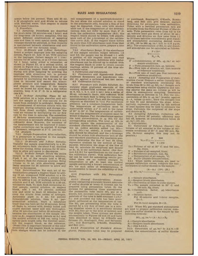
5. A ppara tu s.5.1 D etec to r Cell. Figure D1 is a drawing

of a typical detector cell showing flow paths of gases, th e mixing zone, and placement of th e photom ultiplier tube. O ther flow paths in which the air and ethylene streams meet


81% RULES AND REGULATIONS

a t a point near the photom ultiplier tube are also allowable.

5.2 A ir F low m eter. A device capable of controlling air flows between 0-1.5 1/min.

5.3 E th ylen e F low m eter. A device capable of controlling ethylene flows between 0-50ml. /m in. At any flow in th is range, the device should be capable of m aintaining constant flow rate w ithin ± 3 m l./m in.

5.4 A ir In le t F ilter. A Teflon filter capable of removing all particles greater than 5 microns in diameter.

5.5 P h o to m u ltip lie r T ube. A high gain low dark current (not more th an 1 x 10-® ampere) photom ultiplier tube having its maximum gain a t about 430 nm. The fol-lowing tubes are satisfactory: RCA 4507, RCA 8575, EMI 9750, EMI 9524, and EMI 9536.

5.6 H igh V oltage P ow er S u pp ly. Capable of delivering up to 2,000 volts.

5.7 D irec t C u rren t A m plifier. Capable of full scale amplification of currents from 10-1# to 10-7 ampere; an electrometer is commonly used.

5.8 R ecorder. Capable of fu ll scale display of voltages from the DC amplifier. These volt-ages commonly are in the 1 millivolt to 1-volt range.

5.9 O zone Source an d D ilu tio n S ystem . The ozone source consists of a quartz tube in to which ozone-free air is introduced and then irradiated with a very stable low pres-sure mercury lamp. The level of irradiation is controlled by an adjustable alum inum sleeve which fits around the lamp. Ozone concen-trations are varied by adjustm ent of th is sleeve. At a fixed level of irradiation, ozone is produced a t a constant rate. By carefully controlling the flow of air through the quartz tube, atmospheres are generated which con-ta in constant concentrations of ozone. The levels of ozone in the test atmospheres are determined by the neutral buffered potas-sium iodide method (see section 8). This ozone source and dilution system is shown schematically in Figures D2 and D3, and has been described by Hodgeson, Stevens, and Martin.

5.10 A ppara tu s fo r C alibra tion5.10.1 A bsorber. All-glass impingers as

shown in Figure D4 are recommended. The impingers may be purchased from most m a-jor glassware suppliers. Two absorbers in series are needed to insure complete collec-tion of the sample.

5.10.2 A ir P u m p. Capable of drawing 1 liter/m inute through th e absorbers. The pump should be equipped with a needle valve on the inlet side to regulate flow.

5.10.3 T h erm om eter. W ith an accuracy of ±2« C.

5.10.4 B arom eter. Accurate to the nearestmm. Hg.

5.10.5 F low m eter. Calibrated metering de-vice for measuring flow up to 1 liter /m inute w ithin ± 2 percent. (For measuring flow through impingers.)

5.10.6 F low m eter. For measuring airflow past the lamp; m ust be capable of measuring flows from 2 to 15 liters/m inute w ithin ± 5 percent.

5.10.7 Trap. Containing glass wool to pro-tec t needle valve.

5.10.8 V olum etric Flasks. 25, 100, 500,1,000 ml.

5.10.9 B u ret. 50 ml.5.10.10 P ipe ts. 0.5, 1, 2, 3, 4, 10, 25, and

50 ml. volumetric.5.10.11 Erlenmeyer Flasks. 300 ml.5.10.12 S p ec tro p h o to m eter . Capable of

measuring absorbance a t 352 nm. Matched 1-cm, cells should be used.

6. R eagen ts.6.1 E th ylen e. C. P. grade (m inim um ).6.2 C ylinder Air. Dry grade.6.3 A c tiv a te d Charcoal T rap. For filtering

cylinder air.

6.4 P urified W ater.. Used for all reagents. To distilled or deionized water in an all-glass distillation apparatus, add a crystal of potas-sium permanganate and a crystal of barium hydroxide, and redistill.

6.5 .A bsorb in g R eagen t. Dissolve 13.6 g. potassium dihydrogen phosphate (KH2P 04), 14.2 g. anhydrous disodium hydrogen phos-phate (Na2HP04) or 35.8 g. dodecahydrate salt (Na2HP0412H20 ) , and 10.0 g. potassium iodide (KI) in purified water and dilute to1,000 ml. The pH should be 6.8 ±0.2. The solution is stable for several weeks, if stored in a glass-stoppered amber bottle in a cool, dark place.

6.6 S ta n d a rd A rsen ious O xide S o lu tion (0.05 N ). Use primary standard grade arse-nious oxide (As2Os). Dry 1 hour a t 105° C. immediately before using. Accurately weigh2.4 g. arsenious oxide from a small glass- stoppered weighing bottle. Dissolve in 25 ml. 1 N sodium hydroxide in a flask or beaker on a steam bath. Add 25 ml. 1 N sulfuric acid. Cool, transfer quantitatively to a 1,000-ml. volumetric flask, and dilute to volume. No t e : Solution m ust be neutral to litmus, not alkaline.

w t As 20 3 (g.)Normality As203=------- ------------

49.466.7 Starch In d ica to r S o lu tio n (0.2 p er-

c e n t) . T riturate 0.4 g. soluble starch and ap-proximately 2 mg. mercuric iodide (preserva-tive) w ith a little water. Add the paste slowly to 200 ml. of boiling water. Continue boiling un til the solution is clear, allow to cool, and transfer to a glass-stoppered bottle.

6.8 S ta n d a rd Iod ine S o lu tio n (0.05 N ).6.8.1 P repara tion . Dissolve 5.0 g. potas-

sium iodide (KI) and 3.2 g. resublimed iodine (I2) in 10 ml. purified water. When the iodine dissolves, transfer the solution to a 500-ml. glass-stoppered volumetric flask. Dilute to mark w ith purified water and mix tho r-oughly. Keep solution in a dark brown glass- stoppered bottle away from light, and re-standardize as necessary.

6.8.2 S ta n d a rd iza tio n . Pipet accurately 20 ml. standard arsenious oxide solution into a 300-ml. Erlenmeyer flask. Acidify slightly w ith 1:10 sulfuric acid, neutralize with solid sodium bicarbonate, and add about 2 g. ex-cess. T itrate w ith the standard iodine solu-tion using 5 ml. starch solution as indicator. Saturate the solution w ith carbon dioxide near the end point by adding 1 ml, of 1:10 sulfuric acid. Continue th e titra tion to the first appearance of a blue color which per-sists for 30 seconds.

ml. AS2O3 X Normality As2OaNormality L>=--------------------------- ----------

ml. I2

0.9 D ilu ted S ta n d a rd Iodine. Immediately before use, pipet 1 ml. standard iodine solu-tion into a 100-ml. volumetric flask and dilute to volume with absorbing reagent.

7. Procedure.7.1 Instrum ents can be constructed from

the components given here or may be pur-chased. If commercial instrum ents are used, follow th e specific instructions given in the m anufacturer’s manual. Calibrate th e in -strum ent as directed in section 8. Introduce samples into the system under the same con-ditions of pressure and flow rate as are used in calibration. By proper adjustm ents of zero and span controls, direct reading of ozone concentration is possible.

8. C alibration .8.1 K I C alibra tion Curve. Prepare a curve

of absorbance of various iodine solutions against calculated ozone equivalents as follows:

8.1.1 In to a series of 25 ml. volumetric flasks, pipet 0.5, 1, 2, 3, and 4 ml. of diluted standard iodine solution (6.9). D ilute each to th e mark w ith absorbing reagent. Mix thoroughly, and immediately read the ab-sorbance of each a t 352 nm . against unex-posed absorbing reagent as the reference.

8.1.2 Calculate th e concentration of the solutions as total ¿tig. Os as follows:

Total ¿tig. 0„= (N) (96) (V,)N=Normality I2 (see 6.8.2) , meq./ml.Vj=Volume of diluted standard I2 added,

ml. (0.5,1, 2, 3,4) .Plot absorbance versus total ¿tig. O3,

8.2 In s tru m e n t C alibration .8.2.1 G enera tion o f T est A tm ospheres. As-

semble the apparatus as shown in Figure D3. The ozone concentration produced by the generator can be varied by changing the po-sition of the adjustable sleeve. For calibra-tion of am bient air analyzers, th e ozone source should be capable of producing ozone concentrations in the range 100 to 1,000 ¿tig./m.3 (0.05 to 0.5 p.p.m.) a t a flow rate of a t least 5 liters per m inute. At all times the airflow through the generator m ust be great-er th an the total flow required by the sam-pling systems.

8.2.2 S am plin g an d A nalyses o f T est A t-m ospheres. Assemble the KI sampling tra in as shown in Figure D4. Use ground-glass connections upstream from th e impinger. B u tt-to -bu tt connections with Tygon tubing may be used. The manifold distributing the test atmospheres m ust be sampled simul-taneously by the KI sampling tra in and the instrum ent to be calibrated. Check assem-bled systems for leaks. Record the instru -m ent response in nanoamperes a t each concentration (usually six) . Establish, these concentrations by analysis, using the neu-tra l buffered potassium iodide method as follows:.

8.2.2.1 B lank. W ith ozone lamp off, flush the system for several m inutes to remove residual ozone. Pipet 10 ml. absorbing re-agent into each absorber. Draw air from the ozone-generating system through the sam-pling tra in a t 0.2 to 1 lite r/m inu te for 10 minutes. Immediately transfer the exposed solution to a clean 1-cm. cell. Determine the absorbance a t 352 nm. against unexposed absorbing reagent as the reference. If the system blank gives an absorbance, continue flushing the ozone generation system until no absorbance is obtained.

8.2.2.2 T es t A tm osph eres. W ith the ozone lamp operating, equilibrate th e system for about 10 minutes. Pipet 10 ml. of absorbing reagent into each absorber and collect sam-ples for 10 m inutes in the concentration range desired for calibration. Immediately transfer the solutions from the two absorb-ers to clean 1-cm. cells. Determine the ab-sorbance of each a t 352 nm. against unex-posed absorbing reagent as the reference. Add the absorbances of the two solutions to ob-ta in total absorbance. Read to tal ¿tig.Os from the calibration curve (see 8.1). Calculate to -ta l volume of air sampled corrected to ref-erence conditions of 25° C. and 760 mm. Hg. as follows:

P 298Vk =V X---- X--------x 10-3

760 t+ 273Vr = Volume of air a t reference condi-

tions, m .3V = Volume of air a t sampling condi-

tions, liters.P = Barometric pressure a t sampling

conditions, mm. Hg.t = Temperature a t sampling conditions,

"C.10-8= Conversion of liters to m.a


RULEJS AND REGULATIONS 8197Calculate ozone concentration in p.p.m. as

follows:Ag. Oa

p.p.m. Oa=------ X 5.10 X10-4Vb

8.2.3 In s tru m e n t C a lib ra tion C urve. In -strum ent response from the photom ultiplier tube is ordinarily in current or voltage. Plot th e current, . or voltage if appropriate, (y-axis) for the tes t atmospheres against ozone concentration as determined by th e neutral buffered potassium iodide method, inp.p.m . (x-axis).

9, C alcu lations.9.1 If a recorder is used which has been

properly zeroed and spanned, ozone concen-trations can be read directly.

9.2 If the DC amplifier is read directly, th e reading m ust be converted to ozone concentrations using the instrum ent calibra-tion curve (8.2.3).

9.3 Conversion between p.p.m. and ¿tg./ m.3 values for ozone can be made as follows:

Ag. O*p.pjn. O s=---------X5.10X 10-*

m.®10. B ibliograph y.Hodgeson, J. A., Martin, B. E., and Baum-

gardner, R. e :, “Comparison of Chemilumi-nescent Methods for Measurement of At-mospheric Ozone”, Progress in Analytical Chemistry, Vol. V, Plenum Press, 1971.

Hodgeson, J. A., Stevens, R. K., and Martin, B. E., “A Stable Ozone Source Applicable as a Secondary Standard for Calibration of At-mospheric Monitors”, Analysis Instrum enta-tion Symposium, Instrum ent Society of America« Houston, Tex., April 1971.

Nederbragt, G. W., Van der Horst, A., and Van Duijn, J., N ature 206, 87 (1965).

Warren, G. J., and Babcock, G., R ev. Set. In str . 41, 280 (1970).

SAMPLE AIR IN



Appe n d ix E—Re f e r e n c e Me t h o d f o r De t e r -m in a t io n o f Hy d r o c a r b o n s Co r r e c t e d f o rMe t h a n e

1. P rin cip le an d A p p lica b ility .1.1 Measured volumes of air are^ delivered

semicontinuously (4 to 12 times per hour) to a hydrogen flame ionization detector to measure its to tal hydrocarbon (THCT) con-ten t. An aliquot of th e same air sample is introduced into a stripper column which re-moves water, carbon dioxide, hydrocarbons other th an methane, and carbon monoxide. Methane and carbon monoxide are passed quantitatively to a gas chromatographic col-um n where they are separated. The methane is eluted first, and is passed unchanged through a catalytic reduction tu b e into th e flame ionization detector. The carbon monox-ide is eluted in to . the catalytic reduction tube where it is reduced to m ethane before passing through the flame ionization de-tector. Between analyses the stripper column is backflushed to prepare i t for subsequent analysis. Hydrocarbon concentrations cor-rected for methane are determined by sub-tracting the methane value from the to tal hydrocarbon value. *

Two modes of operation are possible: (1) A complete chromatographic analysis show-ing the continuous ou tpu t from th e detector for each sample injection; (2) The system is programed for autom atic zero and span to display selected band widths of the chromatogram. The peak height is then used

„ as the measure of the concentration. The former operation is referred to as the chro-matographic or spectro mode and the la tter as the barographic or “norm al” mode de-pending on the make of analyzer.

1.2 The method is applicable to the semi- continuous measurement of hydrocarbons corrected for methane in am bient air. The carbon monoxide measurement, which is simultaneously obtained in th is method, is not required in making measurements of hydrocarbons corrected for m ethane and will not be dealt with here.

2. R ange and S e n s itiv ity .2.1 Instrum ents are available w ith vari-

ous range combinations. For atmospheric analysis the THC range is 0-13.1 mg./m.® (0-20 p.pm .) carbon (as CHJ and the m eth -ane range is 0-6.55 mg/m.® (0-10 p.p.m .). For special applications, lower ranges are avail-able and in these applications the range for THC is 0-1.31 mg./m.® (0-2 p.p.m.) carbon (as CHJ and for methane the range is 0-1.31 mg./m.® (0-2p.pna.).

2.2 For the higher, atmospheric analysis ranges the sensitivity for THC is 0.065 mg./m.® (0.1 p.p.m.) carbon (as CH4) and for methane the sensitivity is 0.033 mg./m.® (0.05 p.p.m.). For th e lower, special analysis ranges the sensitivity is 0.016 mg./m.® (0.025 p.pm .) for each gas.

3. In terferences.3.1 No interference in the methane measr

urem ent has been observed. The THC meas-urem ent typically includes all or a portion of w hat is generally classified as the air peak interference. This effect is minimized by proper plumbing arrangements or is ne-gated electronically.

4. Precision, A ccuracy, an d S ta b ility .4.1 Precision determined w ith calibra-

tion gases is +0.5 percent of full scale in the higher, atmospheric analysis ranges.

4.2 Accuracy is dependent on instrum ent linearity and absolute concentration of the calibration gases. An accuracy of 1 percent of full scale in the higher, atmospheric anal-ysis ranges and 2 percent of full scale in the lower, special analysis ranges can be obtained.

4.3 Variations in am bient room tempera-tu re can cause changes in performance char-

tacteristics. This is due to shifts in oven tem perature, flow rates, and pressure w ith am bient tem perature change. The instru -m ent should meet performance specifications w ith room tem perature changes of ±3° C. Baseline d rift is autom atically corrected in th e barographic mode.

5. A ppara tu s.5.1 C om m ercia lly A vailab le THC, CHV

a n d CO A n alyzer. Instrum ents should be in -stalled on location and demonstrated, preferably by the manufacturer, or his rep-resentative, to meet or exceed m anufacturer’s specifications and those described in th is method.

5.2 Sam ple In tro d u c tio n S ystem . Pump, flow control valves, autom atic switching valves, and flowmeter.

5.3 F ilter (In -lin e ) . A binder-free, glass- fiber filter w ith a porosity of 3 to 5 microns should be immediately downstream from the sample pump.

6.4 S tr ip p e r or P reco lum n. Located out-side of the oven a t ambient temperature. The column should be repacked or replaced after th e equivalent of 2 m onths of continu-ous operation.

5.5 Oven. For containing the analytical column and catalytic converter. The oven should be capable of m aintaining an elevated tem perature constant w ithin ±0.5® C. The specific tem perature varies w ith instrum ent m anufacturer.

6. R eagen ts .6.1 C om bu stion Gas. Air containing less

th a n 1.3 mg./m.® (2 p.p.m.) hydrocarbon as methane.

6.2 Fuel. Hydrogen or a m ixture of hydro-gen and inert gas containing less th an 0.065 mg./m.® (0.1 p.p.m.) hydrocarbons asmethane.

6.3 C arrier Gas. Helium, nitrogen,, a ir or hydrogen containing less than 0.065 mg./m.® (0.1 p.p.m.) hydrocarbons as methane.

6.4 Z ero Gas. Air containing less th an 0.065 mg./m.® (0.1 p.p.m.) to tal hydrocarbons as methane.

6.5 C alibra tion G ases. Oases needed far linearity checks (peak . heights) are deter-mined by the ranges used. Calibration gases corresponding to 10, 20, 40, and 80F percent of full scale are needed. Gases m ust be pro-vided w ith certification or guaranteed anal-ysis. Methane is used for both th e to tal hydrocarbon measurement and m ethane measurement.

6.6 S pan Gas. The calibration gas corre-sponding to 80 percent of full scale is used to span the instrum ent.

7. Procedure.7.1 Calibrate the instrum ent as described

in 8.1. Introduce sample into th e system under the same conditions of pressure and flow rates as are used in calibration. (The pump is bypassed only when pressurized cyl-inder gases are used.) Figure E l shows a typical flow diagram; for specific operating instructions refer to m anufacturer’s m a n u a l.

8. C alibration .8.1 C alib ra tion Curve. Determine the

linearity of the system for THC and methane in the barographic mode by introducing zero gas and adjusting the respective zeroing con-trols to indicate a recorder reading of zero, introduce the span gas and adjust th e span control to indicate the proper value on the recorder scale. Recheck zero and span un til adjustm ents are no longer necessary. In tro-duce interm ediate calibration gases and plot the values obtained. If a smooth curve is no t obtained, calibration gases may need replace-ment.

9. C alcu lation .9.1 Determine concentrations, of to ta l

hydrocarbons (as CHJ and CH4, directly from th e calibration curves. No calculations are necessary.

9.2 Determine concentration of hydro-carbons corrected for m ethane by subtracting th e m ethane concentration from th e to ta l hydrocarbon concentration.

9.3 Conversion between p.p.m. and mg./ m.® values for to tal hydrocarbons (as CH4) m ethane and hydrocarbons corrected for methane are made as follows:p.p.m. carbon (as CH4= [mg. carbon (as

CHJ/m.®] X1.5310. B ibliograph y.Fee, G., “Multi-Parameter Air Quality

Analyzer”, ISA Proceedings AID/CHEMPID Symposium, Houston, Texas, April 19-2J, 1971.

Villalobos, R., and Chapman, R. L., “A Gas Chromatographic Method for Automatic Monitoring of Pollutants in Ambient Air”, ibid,

Stevens, R. K„ "The Automated Gas Chromatograph as an Air Pollutant Moni-to r”, 1970 Conference on Environmental Toxicology, U.S. Air Force, W right-Patterson Air Force Base, Dayton, Ohio.

Stevens, R. K., and O’Keeffe, A. E., Anal. C hem . 42, 143A (1970).

Schuck, E". A., Altshuller, A. P., Barth, D. S. and Morgan, G.’ B., “Relationship of Hydro-carbons to Oxidants in Ambient Atmos-pheres”, J. A ir P oll. C on t. Assoc. 20, 297—302 (1970).

Stevens, R. K., O’Keeffe, A. E., and Ortman, G. C., “A Gas Chromatographic Approach to th e Semi-Continuous Monitoring of Atmos-pheric Carbon Monoxide and Methane”, Pro-ceedings o r 11th Conference on Methods in Air Pollution on Industrial Hygiene Studies, Berkeley, Calif., March 30-April 1, 1970.

Swinnerton, J . W., Linnenbom, V. J . and Check, C. H., E nviron . Sci. T echnol. 3, 836 (1969).

Williams, I. G., A dvances in C hrom atog-raph y, Giddings, J. C., and Keller, R. A., ed-itors, MarceH Dekker, N.Y. (1968), pp. 178- 182.

Altshuller, A. P., Kopcznski, S. L., Lonne- man, W. A., Becker, T. L. and Slater, R., E nviron . Sai. T echnol. 1, 899 (1967).

Altshuller, A. P., Cohen, I. R., and Purcell, T. C., Can. J. C hem ., 44, 2973 (1966).

DuBois, L., Zdrojewski, A., and Monkman, J . L., J . A ir Poll. C on t. Assoc. 16, 135 (1966).

Ortman, G. C., A nal. C hem . 38, 644-646 (1966).

Porter, K., and Volman, D. H., A nal. C hem . 34, 748-749 (1962).

CTum, W. M., Proceedings, National Anal-ysis Instrum entation Symposium ISA, 1962.

Schwink, A., Hochenberg, H., and Forder- reuther, M., B renn stoff-C hem ie 72, No. 9, 295 (1961).

Instruction Manual for Air Quality Chro-matograph Model 6800, Beckman Instrum ent Co., Fullerton, Calif.

Instruction Manual, Bendix Corp., Ron- ceverte, W. Va.

Instruction Manual, Byron Instrum ent Co., Raleigh, N.C.

MSA Instruction Manual for GC Process Analyzer for Total Hydrocarbon, Methane and Carbon Monoxide, Pittsburgh, Pa.

Monsanto Enviro-Chem System for Total Hydrocarbons, Methane and Carbon Mon-oxide Instruction Manual, Dayton, Ohio.

Union Carbide Instruction Manual for Model 3020 Gas Chromatograph for CO- CH4-T /1 , White Plains, N.Y.

Instruction Manual for 350 F Analyzer, Tracor Inc., Austin, Tex.

FEDERAL REGISTER, V O L 36. NO. 84— FRIDAY, APRIL 30, 1971


ALUMINUM- 6 - in . P EN -R A Y BOX EN CLO SU RE

Figure D3. Ozone calibration air supply, source, âncf manifold system.


Ad

den

da

A. S

ugg

este

d P

erfo

rman

ce

Spe

cifi

cati

ons

for

Atm

osph

eric

An

alyz

ers

for

Hyd

roca

rbon

s C

orre

cted

for

Met

han

e:R

ange

(m

inim

um) _

____

Out

put

(min

imum

) __

_M

inim

um d

etec

tabl

e se

n-si

tivity

___

____

___

____

Zero

dri

ft (

max

imum

)__

Span

dri

ft (

max

imum

)_Pr

ecis

ion

(min

imum

)__

Ope

ratio

nal p

erio

d (m

ini-

mum

) _

____

____

___

Ope

ratin

g te

mpe

ratu

rera

nge

(min

imum

)___

_O

pera

ting

hum

idity

rang

e(m

inim

um)_

____

____

Lin

eari

ty

(max

imum

)__

0-6

p.p.

m. T

HC

.0-

5 p.

p.m

. CH*

.0-

10

mv.

fu

ll sc

ale.

0.1

p.p.

m.

THC

.0.

1 jp

.p.m

. CH4

.N

ot

to

exce

ed

1 pe

rcen

t/24

hour

s.N

ot

to

exce

ed

1 pe

rcen

t/24

hour

s.±0

.5 p

erce

nt.

3 da

ys.

5-40

° C.

10-1

00 p

erce

nt.

1 pe

rcen

t of

ful

l sc

ale.

B.

Su

gges

ted

Def

init

ion

s of

P

erfo

rman

ceS

peci

fica

tion

s:R

ange

—T

he m

inim

um a

nd m

axim

um m

eas-

urem

ent l

imits

.O

utpu

t—E

lect

rica

l si

gnal

whi

ch i

s pr

opor

-tio

nal

to t

he m

easu

rem

ent;

inte

nded

for

co

nnec

tion

to r

eado

ut o

r da

ta p

roce

ssin

g de

vice

s. U

sual

ly e

xpre

ssed

as

mill

ivol

ts o

r m

lllia

mps

ful

l sca

le a

t a g

iven

impe

denc

e.Pu

ll Sc

ale—

The

max

imum

mea

suri

ng l

imit

for a

giv

en ra

nge.

Min

imum

Det

ecta

ble

Sens

itivi

ty—

The

sm

all-

est

amou

nt o

f in

put

conc

entr

atio

n th

at

can

be d

etec

ted

as t

he c

once

ntra

tion

ap-

proa

ches

zer

o.

Acc

urac

y—T

he d

egre

e of

agr

eem

ent

betw

een

a m

easu

red

valu

e an

d th

e tr

ue v

alue

; us

-ua

lly e

xpre

ssed

at

± p

erce

nt o

f fu

ll s

cale

.La

g T

ime—

The

tim

e in

terv

al f

rom

a s

tep

chan

ge i

n in

put

conc

entr

atio

n at

the

in-

stru

men

t in

let

to t

he f

irst

cor

resp

ondi

ng

chan

ge in

the

inst

rum

ent o

utpu

t.T

ime

to 9

0 Pe

rcen

t R

espo

nse—

The

tim

e in

-te

rval

fro

m a

ste

p ch

ange

in th

e in

put c

on-

cent

ratio

n at

the

ins

trum

ent

inle

t to

a

read

ing

of 9

0 pe

rcen

t of

the

ult

imat

e re

-co

rded

con

cent

ratio

n.R

ise

Tim

e (9

0 pe

rcen

t)—

The

int

erva

l be

-tw

een

init

ial

resp

onse

tim

e an

d tim

e to

90

perc

ent

resp

onse

aft

er a

ste

p de

crea

se i

n th

e in

let c

once

ntra

tion.

Zero

Dri

ft—

The

cha

nge

in in

stru

men

t out

put

over

a s

tate

d tim

e pe

riod

, usu

ally

24

hour

s,

of u

nadj

uste

d co

ntin

uous

ope

ratio

n, w

hen

the

inpu

t co

ncen

trat

ion

is z

ero;

us

ually

ex

pres

sed

as p

erce

nt fu

ll s

cale

.Sp

an D

rift

—T

he c

hang

e in

Ins

trum

ent

out-

put

over

a s

tate

d tim

e pe

riod

, us

ually

24

hour

s, o

f una

djus

ted

cont

inuo

us o

pera

tion,

w

hen

the

inpu

t co

ncen

trat

ion

is a

sta

ted

upsc

ale

valu

e; u

sual

ly e

xpre

ssed

as

perc

ent

full

scal

e.Pr

ecis

ion—

The

deg

ree

of a

gree

men

t be

twee

n re

peat

ed m

easu

rem

ents

of

the

sam

e co

n-ce

ntra

tion.

It

is e

xpre

ssed

as

tbs

aver

age

devi

atio

n of

the

sin

gle

resu

lts f

rom

the

m

ean.

Ope

ratio

nal

Peri

od—

The

per

iod

of t

ime

over

w

hich

the

ins

trum

ent

can

be e

xpec

ted

to

oper

ate

unat

tend

ed w

ithin

spec

ific

atio

ns.

Noi

se—

Spon

tane

ous

devi

atio

ns f

rom

a m

ean

outp

ut n

ot c

ause

d by

inp

ut c

once

ntra

tion

chan

ges.

FED

ERAL

REG

ISTE

R, V

OL.

36

,

Inte

rfer

ence

—A

n un

desi

red

posi

tive

or n

ega-

tive

outp

ut c

ause

d by

a s

ubst

ance

oth

er

than

the

one

bein

g m

easu

red,

in

terf

eren

ce E

quiv

alen

t—T

he p

ortio

n of

in-

dica

ted

inpu

t co

ncen

trat

ion

due

to t

he

pres

ence

of a

n in

terf

èren

t.O

pera

ting

Tem

pera

ture

Ran

ge—

The

rang

e of

am

bien

t te

mpe

ratu

res

over

whi

ch t

he i

n-st

rum

ent w

ill m

eet a

ll pe

rfor

man

ce s

peci

fi-ca

tions

.

Ope

ratin

g H

umid

ity

Ran

ge—

The

ra

nge

of

ambi

ent

rela

tive

hum

idity

ove

r w

hich

the

in

stru

men

t w

ill

mee

t al

l pe

rfor

man

ce

spec

ific

atio

ns.

Lin

eari

ty—

The

max

imum

dev

iatio

n be

twee

n an

ac

tual

in

stru

men

t re

adin

g an

d th

e re

adin

g pr

edic

ted

by a

str

aigh

t lin

e dr

awn

betw

een

uppe

r and

low

«: c

alib

ratio

n po

ints

.

APP

END

IX P

—R

EFER

ENC

E M

ETH

OD

FO

RTH

E D

ETER

MIN

ATI

ON

O

F N

ITR

OG

END

IOX

IDE

IN

THE

ATM

OSP

HER

E (2

4-H

OU

R S

AM

PLIN

G M

ETH

OD

)1.

Pri

nci

ple

and

App

lica

bili

ty.

1.1

Nitr

ogen

dio

xide

is

colle

cted

by

bub-

blin

g ai

r th

roug

h a

sodi

um h

ydro

xide

sol

u-ti

on t

o fo

rm a

sta

ble

solu

tion

of s

odiu

m

nitr

ite. T

he n

itri

te io

n pr

oduc

ed d

urin

g sa

m-

plin

g is

det

erm

ined

col

orlm

etrl

cally

by

reac

t-in

g th

e ex

pose

d ab

sorb

ing

reag

ent

with

ph

osph

oric

ac

id,

sulf

anila

mid

e,

and

N-l

- na

phth

ylet

hyle

nedi

amin

e di

hydr

ochl

orid

e.1.

2 T

he m

etho

d is

app

licab

le to

col

lect

ion

of 2

4-ho

ur s

ampl

es i

n th

e fie

ld a

nd s

ub-

sequ

ent a

naly

sis

in th

e la

bora

tory

.2.

Ran

ge a

nd

Sen

siti

vity

.

2.1

The

ran

ge o

f th

e an

alys

is is

0.0

4 to

1.5

ag

. N

Oj/m

l. W

ith 6

0 m

l. ab

sorb

ing

reag

ent

and

a sa

mpl

ing

rate

of

200

ml./

min

. fo

r 24

ho

urs,

the

ran

ge o

f th

e m

etho

d is

20-

740

fig.

/m.3

(0.

01-0

.4 p

.p.m

.) ni

trog

en d

ioxi

de.

2.2

A c

once

ntra

tion

of 0

.04

ng.

NO

,/ml.

will

pr

oduc

e an

ab

sorb

ance

of

0.0

2 us

ing

1-cm

. ce

lls.

3. I

nte

rfer

ence

s.3.

1 T

he i

nter

fere

nce

of s

ulfu

r di

oxid

e is

el

imin

ated

by

conv

ertin

g it

to

sulf

uric

aci

d w

ith h

ydro

gen

pero

xide

bef

ore

anal

ysis

. (I

)4.

Pre

cisi

on,

Acc

ura

cy,

and

Sta

bili

ty.

4.1

The

rel

ativ

e st

anda

rd d

evia

tions

are

14

.4 p

erce

nt a

nd 2

1.5

perc

ent

at n

itrog

en

diox

ide

conc

entr

atio

ns o

f 14

0 n

g./m

? (0

.072

p.

p.m

.) an

d 20

0 /¿

g./m

.3 (0

.108

p.p

.m.)

, res

pec-

tivel

y, b

ased

on

an a

utom

ated

ana

lysi

s of

1 I, 84

—FR

IDA

Y, A

PRIL

30,

19

71



samples collected from a standard test a t-mosphere. Precision would probably be dif-ferent when the analysis is performed manually.

4.2 No accuracy data are available.4.3 Samples are stable for a t least 6 weeks.5. A ppara tu s.5.1 Sam plin g . See Figure FI.5.1.1 A bsorber. Polypropylene tubes 164 x

32 mm., equipped w ith polypropylene two- port closures.* Rubber stoppers cause high and varying blank values and should not be used. A gas dispersion tube w ith a fritted end of porosity B (70-100 /am. maximum pore diameter) is used.

5.1.1.1 M easu rem en t o f M axim um Pore D iam eter o f F rit. Carefully clean the fr it w ith dichromate-concentrated sulfuric ad d clean-ing solution and rinse well w ith distilled water. Insert through one hole of a two-hole rubber stopper and install in a tes t tube con-tain ing suffident distilled water to cover the fritted portion. A ttach a vacuum source to th e other hole of th e rubber stopper and measure the vacuum required to draw the first perceptible stream of air bubbles through th e frit. Apply the following equation:

. „ ■ 30smaximum pore diameter, /iim. = —s=Surface tension of water in dynes/cm.

a t the tes t tem perature (73 a t 18° C., 72 a t 25* C., and 71 at 31" C.).

P=M easured vacuum, mm. Hg.5.1.2 P robe. Teflon, polypropylene, or

glass tube w ith a polypropylene or glass fu n -nel a t th e end and a membrane filter to pro-tect th e frit. Replace filter after collecting five samples, or more often as indicated by visual observation of the loading.

5.1.3 Flow C on tro l D evice. Calibrated 27- gauge hypodermic needle, three-eighths of an inch long to m aintain a flow of approxi-mately 0.2 liter/m inute. The needle should be protected by a membrane filter. Change filter after collecting 10 samples.

5.1.4 A ir P u m p. Capable of maintaining a flow of 0.2 liter/m inute through the ab-sorber, and a vacuum of 0.7 atmosphere.

5.1.5 C alibra tion E q u ip m en t. Glass flow-meter for measuring airflows up to approxi-mately 275 m l./m in. w ithin ± 2 percent, stopwatch, and precision wet test meter (1 liter/revolution).

5.2 A nalysis.5.2.1 V o lu m etric F lasks. 50, 100, 200, 250,

500, 1,000 ml.5.2.2 G ra d u a ted C ylinder. 1,000 ml.5.2.3 P ip e ts . 1, 2, 5, 10, 15 ml. volumetric;

2 ml., graduated in 1/10 ml. intervals.5.2.4 T est T ube.5.2.5 S p e c tro p h o to m e ter o f C olorim eter.

Capable of measuring absorbance a t 540 nm. Bandwidth is not critical.

6. R eagen ts .6.1 S am plin g .6.1.1 A bsorb in g R eagen t. Dissolve 4.0 g.

sodium hydroxide in distilled water and dilute to 1,000 ml.

6.2 A nalysis.6.2.1 Su lfan ilam ide. Dissolve 20 g. sul-

fanilamide in 700 ml. distilled water. Add, w ith mixing, 50 ml. concentrated phosphoric acid (85 percent) and dilute to 1,000 ml. This solution is stable for a m onth if refrigerated.

6.2.2 NEDA S o lu tion . Dissolve 0.5 g. N -l- naphthylethylenediam ine dihydrochloride in distilled water. This solution is stable for a m onth if refrigerated and protected from light.

6.2.3 H ydrogen Peroxide. Dilute 0.2 ml. 30 percent hydrogen peroxide to 250 ml. w ith distilled water. This solution may be used for a m onth if protected from light.

6.2.4. S ta n d a rd N itr ite So lu tion . Dissolve sufficient desiccated sodium nitrite (NaNOi,

assay of 97 percent or greater) and dilute w ith distilled water to 1,000 ml. so th a t a solution containing 1,000 Ag- NOj/ml. is ob-tained. The am ount of NaNOi to use is cal-culated as follows:

_ 1.500G = —-— X 100 AG =A m ount of NaN02, g.

1.500=Gravimetric factor in converting NOa into NaN02.

A= Assay, percent.7. P rocedure.7.1 Sam pling. Assemble th e sampling

tra in as shown in Figure FI. Add 50 ml. absorbing reagent to the absorber. Disconnect funnel, insert calibrated flowmeter, and measure flow before sampling. If flow rate before sampling is less th an 85 percent of needle calibration, check for leak or change filters as necessary. Remove flowmeter and replace funnel. Sample for 24 hours from m idnight to midnight and measure flow a t end of sampling period.

7.2 A nalysis. Replace any water lost by evaporation during sampling. Pipet 10 ml. of the collected sample into a test tube. Add 1.0 ml. hydrogen peroxide solution, 10.0 ml. sulfanilamide solution, and 1.4 ml. NEDA solution w ith thorough mixing after the addition of each reagent. Prepare a blank in th e same m anner using 10 ml. absorbing reagent. After a 10-minute color-development interval, measure the absorbance a t 540 mm. against th e blank. Read Ag. NOj/ml. from standard curve (Section 8.2).

8. C alibra tion an d Efficiencies.8.1 Sam plin g.8.1.1 C alibra tion o f F low m eter. Using a

wet test meter and a stopwatch, determine the rates of air flow (m l./min.) through the flowmeter a t several ball positions. Plot ball positions versus flow rates.

8.1.2 C alibra tion o f H ypoderm ic Needle. Connect the calibrated flowmeter, the needle to be calibrated, and the source of vacuum in such a way th a t the direction of airflow through the needle is the same as in the sampling train . Read th e position of the ball and determine flow rate in m l./m in. from the calibration chart prepared in 8.1.1. Reject all needles no t having flow rates of 190 to 210 m l./m in. before sampling.

8.2 C alib ra tion Curve. D ilute 5.0 ml. of the 1,000 Ag. NOj/ml. solution to 200 ml. with absorbing reagent. This solution' con-tains 25 Ag- NOj/ml. Pipet 1, 2, 5, and 15 ml. of the 25 Ag. NOj/ml. solution into 50-, 50-, 100-, and 250-ml. volumetric flasks and dilute to the mark with absorbing reagent. The solutions contain 0.50, 1.00, 1.25, and 1.50 Ag- NOj/ml., respectively. Run standards as instructed in 7.2. Plot absorbance vs. Ag- NOj/ml.

8.3 Efficiencies. An overall average effi-ciency of 35 per cent was obtained from test atmospheres having nitrogen dioxide con-centrations of 140 Ag./m.3 and 200 Ag./m.3 by automated analysis.(2)

9. C alcu lation .9.1 Sam plin g.9.1.1 Calculate volume of air sampled.

n 1 WV = XTX10-*2

V= Volume of air sampled, m.*Fj=M easured flow rate before sampling,

m l./m in.F2= Measured flow rate after sampling,

m l./m in.T = Time of sampling, min.

10-®=Conversion of ml. to m.*9.2 Calculate the concentration of n itro-

g en dioxide as Ag. N02/m .3

Ag. N02/m .3=(Ag. NOj/ml.) X50

VX 0.35 ~(Ag. NOj/ml.) X 143

V5 0 = Volume of absorbing reagent used in

sampling, ml.V=Volume of air sampled, m*

0.35=Efficiency."9.2.1 If desired, concentration of nitrogen

dioxide may be calculated as p.p.m. N 02. p.p.m .= (Ag. N02/m .3) X5.32 X10-*

10. R eferences.(1) Jacobs, M. B., and Hochheiser, S., “Con-

tinuous Sampling and Ultramicro-determ ination of Nitrogen Dioxide in Air", A nal. C hem ., 30 426 (1958).

(2) Purdue, L. J., Dudley, J . E., Clements,J. B., and Thompson, R. J., “Studies in Air Sampling for Nitrogen Dioxide,” I. A reinvestigation of the Jacobs- Hochheiser Reagent. In Preparation.

MEMBRANE FILTER MEMBRANE FILTER

♦Available from Bel-Art Products, Pequan- nock, N.J.

Figure F I . Sampling train.[FR Doc.71-6142 Filed 4-29-71;8:51 am]


Date post:	01-Dec-2021
Category:	Documents
Upload:	others
View:	3 times
Download:	0 times

8186 RULES AND REGULATIONS Title 42— PUBLIC HEALTH

Documents