8.Stat

7/29/2019 8.Stat

http://slidepdf.com/reader/full/8stat 1/56

4.1. DESCRIPTIVE STATISTICS

For the research, descriptive statistics include the numbers, charts and graphs used to describe,

organize and present data on each variable. For the research eight variables were determined:

Lenders trustworthy, Assurance of Credit Risk, Requirement, types of loan, New Loans, Loans

against documentary bills payment, factor for providing a customer loan, significant is dependent

variables. Values of the variables were derived after averaging three questions under each

variable. Mean, standard deviation, variance, minimum & maximum value for each value is

shown in the following table.

TABLE 1: Descriptive Statistics of all variables

Descriptive Statistics

N Minimum Maximum Mean Std. Deviation Variance

MEAN of Lenders

Trustworthy

100 2.29 4.43 3.6714 .44323 .196

MEAN of Assurance of

Credit Risk

100 2.00 4.83 3.5183 .53070 .282

MEAN of Credit Analysis 100 1.60 4.80 3.6480 .65697 .432

MEAN of Consideration

Factor

100 1.60 4.60 3.4440 .59396 .353

MEAN of Significance 100 2.50 4.67 3.8333 .52384 .274

Valid N (list wise) 100

This table provides the basic statistical information about the data set, such as showing the mean

response for average of five questions for each variable individual questions and its deviation

from the mean. For this information, for instance we find that the among the 100 participants

72were male and 28 were female which is 72% male & 28% female. Participants of the research

came from various age groups. Age range of the participants is 20 to above 40. But most of the

participants belongs to the age group 25 -34 & 31 -35. These descriptive statistics of the entire

data set has been represented in Table 1 (given in Appendix).

4.2. Frequency distribution and charts

Graphical representation of data and frequency distribution:

7/29/2019 8.Stat


Table4.2.1: Gender of the respondents

Frequency Percent Valid Percent Cumulative Percent

Valid Male 72 72.0 72.0 72.0

Female 28 28.0 28.0 100.0

Total 100 100.0 100.0

Figure 4.2.1: Diagram showing the frequency distribution of gender

There were 100 respondents of which 72 were male and 28 were female. These respondents are

all employees and customers in BASIC Bank Limited from various departments in various

branches.

From the various branches we found that the numbers of male employees are more than the

female employees.

Table 4.2.2: Respondents Age Distribution


Valid

25-30 38 38.0 38.0 38.0

35-40 37 37.0 37.0 75.0

72

28

7/29/2019 8.Stat


31-35 15 15.0 15.0 90.0

40 & above 10 10.0 10.0 100.0

Total 100 100.0 100.0

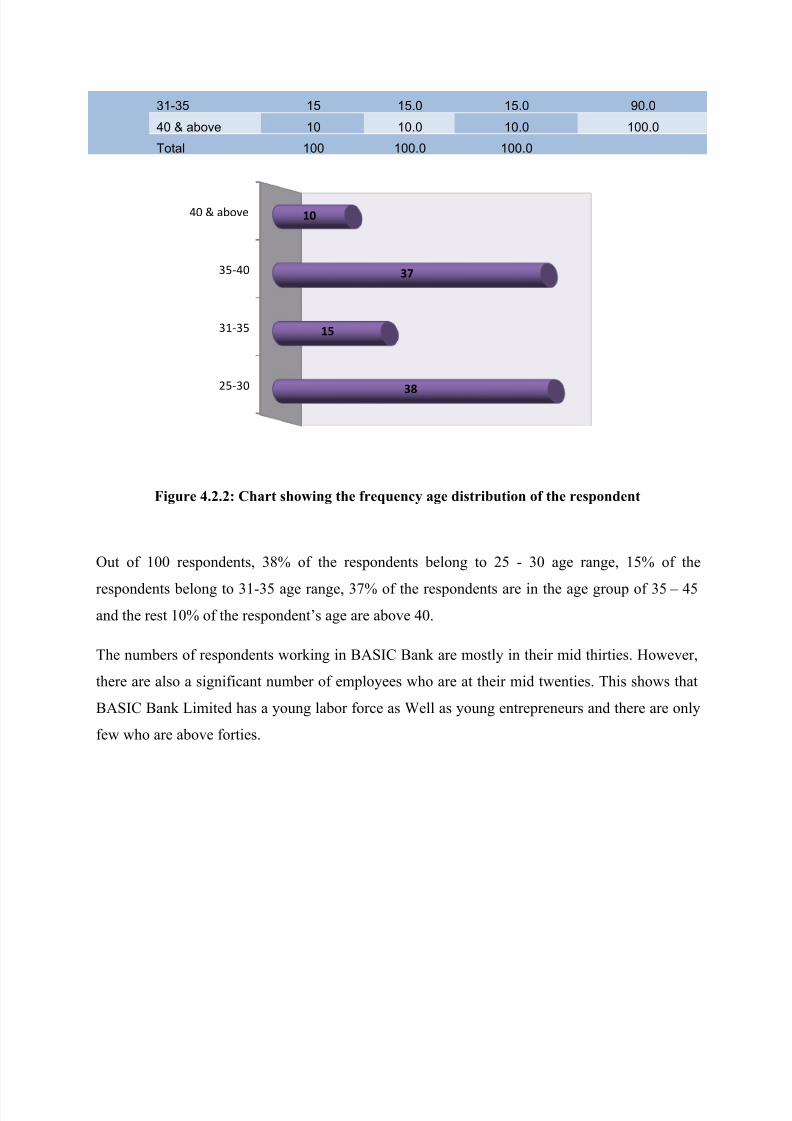
Figure 4.2.2: Chart showing the frequency age distribution of the respondent

Out of 100 respondents, 38% of the respondents belong to 25 - 30 age range, 15% of the

respondents belong to 31-35 age range, 37% of the respondents are in the age group of 35 – 45

and the rest 10% of the respondent’s age are above 40.

The numbers of respondents working in BASIC Bank are mostly in their mid thirties. However,

there are also a significant number of employees who are at their mid twenties. This shows that

BASIC Bank Limited has a young labor force as Well as young entrepreneurs and there are only

few who are above forties.

38

15

37

10

25-30

31-35

35-40

40 & above

7/29/2019 8.Stat


Figure 4.2.3: Chart showing the frequency Educational background distribution of the

respondents

Of the respondents 29% of above respondents education background are science, 27% are from

commerce education background, 31% respondents are from Arts, and 10% are vocational and

others 3%.

Employees of BASIC bank Limited are from various educational backgrounds. From the 50

sample size, 16 employees are from Arts, Science and Commerce are almost same 14 and 13

each. Only a few employees are from vocational and others types of educational background.

29

27

31

10

3

0

5

10

15

20

25

30

35

0 1 2 3 4 5 6

Table 4.2.3: Respondents Educational background


Valid

science 29 29.0 29.0 29.0

commerce 27 27.0 27.0 56.0 Arts 31 31.0 31.0 87.0

vocational 10 10.0 10.0 97.0

others 3 3.0 3.0 100.0

Total 50 100.0 100.0

7/29/2019 8.Stat


Table 4.2.5: Lenders Potential


Valid strongly Disagree 5 10.0 10.0 10.0

Disagree 19 38.0 38.0 48.0

Neutral 14 28.0 28.0 76.0

agree 7 14.0 14.0 90.0

strongly agree 5 10.0 10.0 100.0

Total 50 100.0 100.0

Figure 4.2.5: Showing the frequency distribution of Lenders Potential

Of the 50 respondents 10% strongly agreed to the satisfaction in the current IT system used in the

current process, 14% agreed, 28% are neutral about the satisfaction with the IT system, 38%

disagreed that there is no satisfaction and 10% strongly disagreed.

0

5

10

15

20

25

30

35

40

strongly

Disagree

Disagree Neutral agree strongly

agree

7/29/2019 8.Stat


Most of the employees are unconcerned about the Lenders potential. Although a significant

number of employees are satisfied with their current process they use. It is because, employees

aren’t aware of the different method or software used in the job.

Figure 4.2.6: Showing the frequency distribution of Lenders Honesty

Of the 100 respondents 20% strongly agreed to the current process, 56% agreed, 12% are neutral

about the satisfaction with the existing method system while 10% disagreed and thought they

shouldn’t take it as a and 2% strongly disagreed.

0

10

20

30

40

50

60

strongly

DisagreeDisagree

Neutralagree

strongly

agree

Table4.2.6: Lenders Honesty

Frequency Percent Valid Percent Cumulative

Percent


Disagree 5 10.0 10.0 12.0

Neutral 6 12.0 12.0 24.0

agree 28 56.0 56.0 80.0

strongly agree 10 20.0 20.0 100.0

Total 50 100.0 100.0

7/29/2019 8.Stat


Maximum no. of employees is not satisfied with the existing system. There is a significant no. of

employees think the Existing system could hinder employees’ productivity.

Figure 4.2.7: Showing the frequency distribution of Asset and Liability

Of the 100 respondents 22% strongly agreed that the current method by the management used decrease

overall efficiency, 52% agreed, 12% are neutral with the current process, 8% disagreed that Existing

system does not decrease overall efficiency and 5% strongly disagreed.

6

812

52

22

0

10

20

30

40

50

60

strongly

Disagree

Disagree Neutral agree strongly agree

Table 4.2.7: Asset and Liability



Disagree 4 8.0 8.0 14.0

Neutral 6 12.0 12.0 26.0

agree 26 52.0 52.0 78.0

strongly agree 11 22.0 22.0 100.0

Total 50 100.0 100.0

7/29/2019 8.Stat


According to a large number of respondents, they are not happy with the liability. They think that existing

liability decrease overall efficiency.

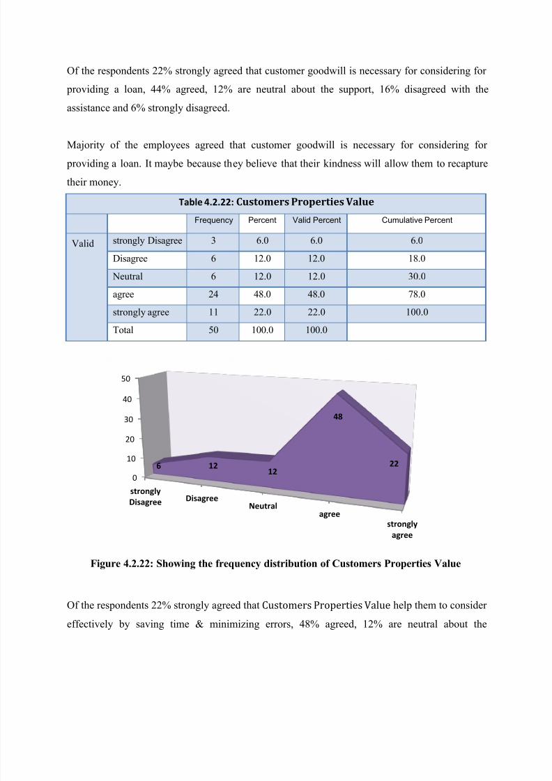
Figure 4.2.8: Showing the frequency distribution of Profitability

Of the respondents 34% strongly agreed to the improvement of profitability is needed when

examining a new client, 42% agreed, 10% are neutral, 12% disagreed that there is no need to

change that formula and 2% strongly disagreed.

strongly Disagree,

1

Disagree, 6

Neutral, 5

agree, 21

strongly agree, 17

Table 4.2.8: Profitability



Disagree 6 12.0 12.0 14.0

Neutral 5 10.0 10.0 24.0

agree 21 42.0 42.0 66.0

strongly agree 17 34.0 34.0 100.0

Total 50 100.0 100.0

7/29/2019 8.Stat


Majority of the employees said that the practice used in their current system doesn’t need to be

improved. However, a significant number of employees feel the need of improvement in their

current structure.

Figure 4.2.9: Showing the frequency distribution of Timely Repayment

Of the respondents 26% strongly agreed to the timely repayment is needed to ensure granting

further sanction, 44% agreed, 18% are neutral about the improvement, 8% disagreed that there is

no need for enhancement and 4% strongly disagreed.

4

8

18

44

26

0

5

10

15

20

25

30

35

40

45

50

strongly

Disagree


Table4.2.9: Timely Repayment



Disagree 4 8.0 8.0 12.0

Neutral 9 18.0 18.0 30.0

agree 22 44.0 44.0 74.0

strongly agree 13 26.0 26.0 100.0

Total 50 100.0 100.0

7/29/2019 8.Stat


Most of the employees said that timely repayment method can be improved if there is an

improvement loan processing. It is because the current system used by the employees of BASIC

Bank Limited isn’t satisfactory for which their skills aren’t able to enhance.

Figure 4.2.10: Showing the frequency distribution of Supervision

Of the respondents 32% strongly agreed to perform effectively by saving time, 36% agreed, 14%

are neutral about the performance, 10% disagreed that the current system helps to perform

effectively and 7% strongly disagreed.

8

10

14

3632

0

5

10

15

20

25

30

35

40

strongly

Disagree


Table 4.2.10: Supervision



Disagree 5 10.0 10.0 18.0

Neutral 7 14.0 14.0 32.0

agree 18 36.0 36.0 68.0

strongly agree 16 32.0 32.0 100.0

Total 50 100.0 100.0

7/29/2019 8.Stat


From the graph, it can be seen that most of the employees believe that improvement in

supervision doesn’t help them to perform effectively by saving time. It is because they are not

aware of other method of doing the work. Hence, the employees don’t know the effect of

business process reengineering on the performance of their work.

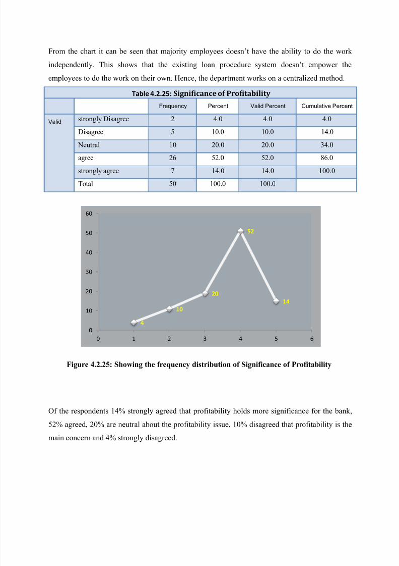
Table 4.2.11: Monitoring



Disagree 4 8.0 8.0 12.0

Neutral 9 18.0 18.0 30.0

agree 24 48.0 48.0 78.0

strongly agree 11 22.0 22.0 100.0

Total 50 100.0 100.0

Figure 4.2.11: Showing the frequency distribution of Monitoring

Of the respondents 22% strongly agreed to perform efficiently by minimizing errors monitoring

frequently, 48% agreed, 18% are neutral about the performance, 7% disagreed that monitoring

frequently helps to perform efficiently and 4% strongly disagreed.

48

18

48

22

0

5

10

15

20

25

30

35

40

45

50

0 1 2 3 4 5 6

7/29/2019 8.Stat


From the graph, it can be seen that most of the employees believe that improvement in

monitoring process doesn’t help them to perform efficiently by minimizing errors. It is because

they are not aware of other method of doing the work. Hence, the employees don’t know the

effect of business process reengineering on the performance of their work.

Table 4.2.12: Credit Policy



Disagree 20 40.0 40.0 54.0

Neutral 10 20.0 20.0 74.0

agree 10 20.0 20.0 94.0


Total 50 100.0 100.0

Figure 4.2.12: Showing the frequency distribution of Credit Policy

Of the respondents 6% strongly agreed of their satisfaction with the credit policy they maintain

in the current process, 20% agreed, 20% are neutral about the satisfaction, 40% disagreed with it

and 14% strongly disagreed.

14

20

20

20

6

0 10 20 30 40 50

strongly Disagree

Disagree

Neutral

agree

strongly agree

7/29/2019 8.Stat


It can be seen from the graph that the employees aren’t satisfied with credit policy and it needs

reengineering in the current process. The employees believe that there is a need of more strict

policy in their current process in order to enhance their work performance.

Table 4.2.13: Credit Procedure



Disagree 8 16.0 16.0 20.0

Neutral 7 14.0 14.0 34.0

agree 22 44.0 44.0 78.0

strongly agree 11 22.0 22.0 100.0

Total 50 100.0 100.0

Figure 4.2.13: Showing the frequency distribution of Credit Procedure

Of the respondents 22% strongly agreed to the need of Credit Procedure in the unit, 44% agreed,

14% are neutral about the satisfaction, 16% disagreed with more number of skilled employees

and 4% strongly disagreed.

0

10

20

30

40

50

strongly

DisagreeDisagree

Neutralagree

strongly

agree

416

14

44

22

7/29/2019 8.Stat


Majority of the employees agreed and disagreed to the need of more of Credit procedure in the

unit. It maybe because the current employees find addition of new employees to the work as a

threat to their job and other welcomes the help of more techniques as they believe it can enhance

the efficient level of the working environment.

Table 4.2.14: Quality of Credit Portfolio



Disagree 7 14.0 14.0 20.0

Neutral 11 22.0 22.0 42.0

agree 20 40.0 40.0 82.0


Total 50 100.0 100.0

Figure 4.2.14: Showing the frequency distribution of Quality of Credit Portfolio

Of the respondents 6% strongly agreed that Quality of Credit Portfolio are necessary while 40%

agreed, 22% are neutral about the necessity, 14% disagreed with the necessity and 6% strongly

disagreed.

6%14%

22%

40%

18%

strongly Disagree Disagree Neutral agree strongly agree

7/29/2019 8.Stat


From the pie chart, it can be seen that the majority of the employees agreed to the necessity of

Quality of Credit Portfolio to maximize the use of credit disbursement. Since, skilled employees

are able to maximize the use of the credit disbursement then the employees who doesn’t have

any strategic skills.

Table 4.2.15: Continuous Loan



Disagree 7 14.0 14.0 18.0

Neutral 7 14.0 14.0 32.0

agree 25 50.0 50.0 82.0

strongly agree 9 18.0 18.0 100.0Total 50 100.0 100.0

Figure 4.2.15: Showing the frequency distribution of Continuous Loan

Of the respondents 18% strongly agreed that continuous loans are the most effective for the bank

to survive, 50% agreed, 14% are neutral about the effectiveness, 14% disagreed with the

effectiveness by saving time and 4% strongly disagreed.

0 10 20 30 40 50

strongly Disagree

Disagree

Neutral

agree

strongly agree

4

14

14

50

18

7/29/2019 8.Stat


From the graph, it can be seen that majority of the employees are being indifferent about the

continuous loans in their performance through saving time. The employees are aware of the

effect of continuous loans. They believe that they don’t need any other loans and skills to dotheir job.

Table 4.2.16: Demand Loan



Disagree 7 14.0 14.0 16.0

Neutral 5 10.0 10.0 26.0

agree 24 48.0 48.0 74.0strongly agree 13 26.0 26.0 100.0

Total 50 100.0 100.0

Figure 4.2.16: Showing the frequency distribution of Demand Loan

Of the respondents 26% strongly agreed that Demand Loan helps to perform efficiently by

minimizing transaction cost and error, 48% agreed, 10% are neutral about the efficiency, 14%

2

1410

48

26

0

5

10

15

20

25

30

35

40

45

50


7/29/2019 8.Stat


disagreed with the efficiency of demand loan by minimizing transaction cost and error and 2%

strongly disagreed.

It can be seen that majority of the employees are being indifferent about the efficiency of

demand loan in their performance through minimizing errors. The employees are aware of the

effect of demand loan have on their performance of work.

Table 4.2.17: Term Loan



Disagree 4 8.0 8.0 14.0

Neutral 6 12.0 12.0 26.0

agree 22 44.0 44.0 70.0

strongly agree 15 30.0 30.0 100.0

Total 50 100.0 100.0

Figure 4.2.17: Showing the frequency distribution of Term Loan

0

5

10

15

20

25

30

3540

45

strongly

Disagree


6

812

44

30

7/29/2019 8.Stat


Of the respondents 30% strongly agreed that Term loan helps to enhance overall efficiency, 44%

agreed, 12% are neutral about the efficiency, 8% disagreed with the efficiency of term loan and

6% strongly disagreed.

It is shown from the above graph that, most of the employees think that term helps to enhance

their overall efficiency. If they continue sanctioning more term loan, then their overall efficiency

will increase.

Table 4.2.18: New Loans in New Industry



Disagree 6 12.0 12.0 18.0

Neutral 6 12.0 12.0 30.0

agree 22 44.0 44.0 74.0

strongly agree 13 26.0 26.0 100.0

Total 50 100.0 100.0

Figure 4.2.18: Showing the frequency distribution of New Loans in New Industry

6

12 12

44

26

0

5

10

15

20

25

30

35

40

45

50


7/29/2019 8.Stat


Of the respondents 26% strongly agreed that the bank should made immediate sanction if they

have any request for investing in new industry as it can be effective, 44% agreed, 12% are

neutral about the necessity, 12% disagreed with the necessity execution and 6% strongly

disagreed.

From the line graph, it can be seen that the most of the employees agreed to sanction new loans

for new industry. It is because employees feel the needs of sanctioning loans in new industry

could become valuable.

Table 4.2.19: Foreign Currency



Disagree 9 18.0 18.0 24.0

Neutral 12 24.0 24.0 48.0

agree 18 36.0 36.0 84.0


Total 50 100.0 100.0

Figure 4.2.19: Showing the frequency distribution of Foreign Currency

strongly

Disagree, 6

Disagree, 18

Neutral, 24agree, 36

strongly agree,

16

7/29/2019 8.Stat


Of the respondents 16% strongly agreed that foreign currency will increase flexibility and

adaptability that is necessary to compete with other commercial banks, 36% agreed, 24% are

neutral about the flexibility and adaptability, 18% disagreed and 6% strongly disagreed.

Majority of the employees agreed foreign currency will increase the profitability to increase their

performance.

Table 4.2.20: Local Currency



Disagree 5 10.0 10.0 16.0

Neutral 7 14.0 14.0 30.0

agree 23 46.0 46.0 76.0

strongly agree 12 24.0 24.0 100.0

Total 50 100.0 100.0

Figure 4.2.20: Showing the frequency distribution of Local Currency

0

5

10

15

20

25

30

35

40

45

50

strongly

Disagree


610

14

46

24

7/29/2019 8.Stat


Of the respondents 24% strongly agreed that local currency can also prove valuable and 46%

agreed, 14% are neutral about the assistance, 10% disagreed with the assistance in developing

new field and 6% strongly disagreed.

Majority of the employees are agreeing about the growth of local currency. It maybe because

they believe that local currency is mandatory to develop a new route properly.

Table 4.2.21: Customer Goodwill



Disagree 8 16.0 16.0 22.0

Neutral 6 12.0 12.0 34.0

agree 22 44.0 44.0 78.0

strongly agree 11 22.0 22.0 100.0

Total 50 100.0 100.0

Figure 4.2.21: Showing the frequency distribution of Customer Goodwill

0 5 10 15 20 25 30 35 40 45

strongly Disagree

Disagree

Neutral

agree

strongly agree

6

16

12

44

22

7/29/2019 8.Stat


Of the respondents 22% strongly agreed that customer goodwill is necessary for considering for

providing a loan, 44% agreed, 12% are neutral about the support, 16% disagreed with the

assistance and 6% strongly disagreed.

Majority of the employees agreed that customer goodwill is necessary for considering for

providing a loan. It maybe because they believe that their kindness will allow them to recapture

their money.

Table 4.2.22: Customers Properties Value



Disagree 6 12.0 12.0 18.0

Neutral 6 12.0 12.0 30.0

agree 24 48.0 48.0 78.0

strongly agree 11 22.0 22.0 100.0

Total 50 100.0 100.0

Figure 4.2.22: Showing the frequency distribution of Customers Properties Value

Of the respondents 22% strongly agreed that Customers Properties Value help them to consider

effectively by saving time & minimizing errors, 48% agreed, 12% are neutral about the

0

10

20

30

40

50

strongly

Disagree DisagreeNeutral

agree

strongly

agree

6 1212

48

22

7/29/2019 8.Stat


performing effectively by saving time, 12% disagreed with the effective performance and 6%

strongly disagreed.

From the graph, it can be seen that Customers Properties Value help the employees perform

effectively by saving time and minimizing errors. It may be because the employees think that it

saves their time.

Table 4.2.23: Customer Income



Disagree 4 8.0 8.0 16.0

Neutral 10 20.0 20.0 36.0

agree 20 40.0 40.0 76.0

strongly agree 12 24.0 24.0 100.0

Total 50 100.0 100.0

Figure 4.2.23: Showing the frequency distribution of Customer Income

Of the respondents 24% strongly agreed that customer income is efficient for consideration, 40%

agreed, 20% are neutral about it, 8% disagreed with it and 8% strongly disagreed.

0 5 10 15 20 25 30 35 40 45

strongly Disagree

Disagree

Neutral

agree

strongly agree

8

8

20

40

24

7/29/2019 8.Stat


The graph shows that majority of the employees think positive about customer income.. Since

the work perform by employees are centralized they are reluctant to waste more time on making

a formal proposal to the management.

Table 4.2.24: Customers Loan Purpose



Disagree 19 38.0 38.0 50.0

Neutral 13 26.0 26.0 76.0

agree 10 20.0 20.0 96.0


Total 50 100.0 100.0

Figure 4.2.24: Showing the frequency distribution of Customers Loan Purpose

Of the respondents 4% strongly agreed that customers loan purpose increases employees anxiety,

20% agreed, 26% are neutral about the ability to do the work independently, 38% disagreed with

the independence of the work in the current system and 12% strongly disagreed.

0

5

10

15

20

25

30

35

40

strongly

Disagree


agree

12

38

26

20

4

7/29/2019 8.Stat


From the chart it can be seen that majority employees doesn’t have the ability to do the work

independently. This shows that the existing loan procedure system doesn’t empower the

employees to do the work on their own. Hence, the department works on a centralized method.

Table 4.2.25: Significance of Profitability



Disagree 5 10.0 10.0 14.0

Neutral 10 20.0 20.0 34.0

agree 26 52.0 52.0 86.0


Total 50 100.0 100.0

Figure 4.2.25: Showing the frequency distribution of Significance of Profitability

Of the respondents 14% strongly agreed that profitability holds more significance for the bank,

52% agreed, 20% are neutral about the profitability issue, 10% disagreed that profitability is the

main concern and 4% strongly disagreed.

4

10

20

52

14

0

10

20

30

40

50

60

0 1 2 3 4 5 6

7/29/2019 8.Stat


Majority of the employees agreed that profitability holds more significance. Employees believe

that profitability can help them to achieve their goal.

Table 4.2.26: Significance of Liquidity



Disagree 7 14.0 14.0 20.0

Neutral 9 18.0 18.0 38.0

agree 22 44.0 44.0 82.0


Total 50 100.0 100.0

Figure 4.2.26: Showing the frequency distribution of Significance of Liquidity

Of the respondents 18% strongly agreed that liquidity holds more significance for the bank to

perform effectively by saving time, 44% agreed, 18% are neutral about the effective performance

by saving time, 14% disagreed that profitability holds more significance than liquidity and 5%

strongly disagreed.

Most of the employees agreed that liquidity carries more importance and helps to perform

effectively by saving time. It allows banks to have more freedom to do their work as there is no

dependence on others.

314

18

44

18

strongly Disagree

Disagree

Neutral

agree

strongly agree

7/29/2019 8.Stat


4.3 Cross tabulation Analysis

Table 4.3.1: Cross tabulation of Gender & Lenders Potential

Count

Satisfied with the Lenders Potential Totalstrongly

Disagree


Gender Male 7 26 21 11 7 72

Female 2 12 7 4 3 28

Total 9 38 28 15 10 100

From the above cross tabulation analysis, 36% respondents of Male and 42.8% female which

mean 26 Male employees out of 72 and 12 Female employees out of 28 are disagree with the

existing trustworthy system in BASIC Bank Limited. Overall 38 respondents out of 100 are not

satisfied with the existing system.

Table 4.3.2: Cross tabulation of Age & Lenders Asset and Liability Worth

Count

Lenders Asset and Liability plays a vital role Total

strongly

Disagree


Age 25-30 3 5 3 18 9 38

35-40 2 2 4 23 6 37

31-35 0 0 2 7 6 15

40 & above 0 2 3 3 2 10

Total 5 9 12 51 23 100

From the above cross tabulation analysis, 47% respondents of 25-30 age group, 46% of

respondent age group 31-35, 62% of respondent from age group 35-40 and 30% respondent of 40

& above age group agree with the Asset and Liability practice in BASIC bank. In total 51

employees out of 100, think that existing method of BASIC bank decrease overall efficiency.

Table 4.3.3: Cross tabulation of Education & Profitability

7/29/2019 8.Stat


Count

Profitability Total

strongly

Disagree


Education science 0 4 3 11 11 29

commerce 0 4 2 9 12 27

Arts 1 4 3 16 7 31

vocational 0 0 1 5 4 10

others 0 1 1 1 0 3

Total 1 13 10 42 34 100

From the above cross tabulation analysis, 37% respondents of science, 33% of respondent

commerce, 50% of respondent from Arts group, and 50% respondent of vocational group are

agree that the existing system can be improved in BASIC bank. In total 42 employees out of 100,

think that existing method of BASIC Bank can be improved.

Table 4.3.4: Cross tabulation of Education & Customer Goodwill

Count

Customer Goodwill Total


Age Range of

therespondents

Science 1 8 8 19 8 44

Commerce 2 1 4 0 3 10Arts 1 1 2 6 0 10

Vocational 1 3 7 7 4 22

Others 1 2 1 8 2 14

Total 6 15 22 40 17 100

From the above cross tabulation analysis, age range of 43% respondents of science, 60% of

respondents of commerce, 30% of respondent from arts, and 50% respondent of vocational are

agree with the customers goodwill that are essential to maximize the use of profitability of

BASIC Bank. In total 40 employees out of 100, think that goodwill are essential to maximize the

profit.

7/29/2019 8.Stat


Table 4.3.5: Cross tabulation of Gender & New Loans in new industry

Count

New Loans in new industry Total

strongly

Disagree


Gender Male 5 7 8 36 16 72

Female 1 4 4 8 11 28

Total 6 11 12 44 27 100

From the above cross tabulation analysis, 50% respondents of Male and 33.33% female which

mean 26 Male employees out of 72 and 12 Female employees out of 28 are disagree that the

new loans should be sanctioned for new industry in BASIC Bank. Overall 44 respondents out of

100 are thinking that new loans should be made available to increase the efficiency of BASIC

Bank.

Table 4.3.6: Cross tabulation of Age & Customer Income

Count

Customer Income Total

strongly

Disagree


agree

Age 25-30 2 4 1 18 13 38

35-40 4 7 9 13 4 37

31-35 0 2 1 8 4 15

40 &

above

0 2 1 6 1 10

Total 6 15 12 45 22 100

From the above cross tabulation analysis, 47.36% respondents of 25-30 age group, 53% of

respondent age group 31-35, 35% of respondent from age group 35-40 and 60% respondent of 40

& above age group are agree customer income is necessity to sanction loan in BASIC Bank. In

total 45 employees out of 100, think that Customer income is needed to take under consideration

in BASIC Bank.

7/29/2019 8.Stat


Table 4.3.7: Cross tabulation of Age & Customer Loan Purpose

Count

Customer Loan Purpose Total

stronglyDisagree

Disagree Neutral agree stronglyagree

Age 25-30 4 14 8 8 4 38

35-40 6 12 13 6 0 37

31-35 0 10 2 3 0 15

40 &

above

2 2 3 2 1 10

Total 12 38 26 19 5 100

From the above cross tabulation analysis, 36.84% respondents of 25-30 age group, 66.66% of

respondent age group 31-35, 32% of respondent from age group 35-40, But only 20%

respondent of 40 & above age group are disagree with Existing loan system gives the ability to

do work independently in BASIC Bank. In total 38 employees out of 100, think that existing

structure gives the ability to do work independently in BASIC Bank. It means Existing

management does not give the ability to do work independently.

Table 4.3.8: Cross tabulation of Age & Customers Properties Values

Count

Customers Properties Values Total

strongly

Disagree


agree

Age 25-30 0 3 6 23 6 38

35-40 3 2 9 17 6 37

31-35 0 5 2 6 2 15

40 & above 1 1 2 5 1 10

Total 4 11 19 51 15 100


respondent age group 31-35, 43% of respondent from age group 35-40 and only 50% respondent

of 40 & above age group are agree with Customers Properties Values. In total 51 employees out

of 100, think that Customers Properties Values helps employees reconsider and work

independently in BASIC bank.

7/29/2019 8.Stat


Table 4.3.9: Cross tabulation of Age & Liquidity

Count

Liquidity Total

strongly

Disagree


agree

Age 25-30 3 7 4 15 9 3835-40 2 2 8 18 7 37

31-35 0 0 2 8 5 15

40 & above 0 1 0 5 4 10

Total 5 10 14 46 25 100


respondent age group 31-35, 48% of respondent from age group 35-40 and only 50% respondent

of 40 & above age group are agree with liquidity is more important. Overall 46 employees out of

100, think that Efficiency of bank can be improved if it has high liquidity in BASIC bank.

Table 4.3.10: Cross tabulation of Lenders Potential & Timely Repayment

Count

Timely Repayment Total

strongly

Disagree


agree

Lenders Potential Yes 3 9 8 35 27 82

No 2 2 4 7 3 18

Total 5 11 12 42 30 100

82% of respondent who believe that lenders potential can improve customer efficiency where

67% of them are agree and 32% of them are strongly agree with efficiency is better when

lenders repay timely. On the other hand 18 respondents out of 100 are believed that timely

repayment doesn’t necessarily mean that it has huge potential.

Table 4.3.11: Cross tabulation of Credit Procedure & Profitability

Count

Profitability Total

strongly Disagree Neutral agree strongly

7/29/2019 8.Stat


Disagree agree

Credit Procedure Yes 5 7 7 41 22 82

No 0 2 1 7 8 18

Total 5 9 8 48 30 100

From the above cross tabulation analysis, 50% respondents agree with credit procedure is perfect

to boost employees efficiency. Overall 82 employees out of 100 believe that credit procedure

boost employee’s efficiency in BASIC Bank and 18 respondents believe that credit procedure

hampering employee’s efficiency.

Table 4.3.12: Cross tabulation of Education & Customer IncomeCount

Customer Income Total

strongly

Disagree


Education science 3 1 1 13 11 29

commerc

e

1 1 1 14 10 27

Arts 2 2 4 11 12 31

vocational 0 0 1 5 4 10

others 0 1 0 2 0 3

Total 6 5 7 45 37 100

From the above cross tabulation analysis, 44% respondents of science, 52% of respondent

commerce, 35% of respondent from Arts group, and 50% respondent of vocational group and 2

respondent of others educational background are agree with greater Customers Income speed up

the loan process. In total 45 employees out of 100, think that Education helps to enhance overall

employee’s efficiency in BASIC Bank .

4.4 Chi-Square Analysis

4.4.a Chi-square test between Responsiveness performed by respondent and believes that using it

is related with customer satisfaction.

7/29/2019 8.Stat


H0: Responsiveness is not positively correlated with customer satisfaction

H1: Responsiveness is positively correlated with customer satisfaction

TABLE 4.4.1: Chi-Square Tests between responsiveness performed by respondent and customer

satisfaction

Value df Asymp. Sig. (2-sided)

Pearson Chi-Square 13.086a

4 .011

Likelihood Ratio 13.242 4 .010

Linear-by-Linear Association 3.151 1 .076

a. 4 cells (40.0%) have expected count less than 5. The minimum expected count is 1.80.

Decision: the significance level is lower than 0.05. Therefore null hypothesis should be rejected. So

it can be stated that Responsiveness is positively correlated with customer satisfaction.

4.4.b Chi-square test of Age and necessity of IT training

H0: Age and Lenders Potential are independent

H1: Age and Lenders Potential are dependent

TABLE 4.4.2: Chi-square test of Age and Lenders Potential


Pearson Chi-Square 22.142a 12 .036


Linear-by-Linear Association .147 1 .701

a. 15 cells (75.0%) have expected count less than 5. The minimum expected count is .60.

Decision: the significance level is lower than 0.05. Therefore null hypothesis should be rejected. So

it can be stated that Age and Lenders Potential are independent.

4.4.c Chi-square test of Age and Employee empowerment is needed to improve performance

H0: Age and Supervision is needed to improve performance are independent

H1: Age and Supervision is needed to improve performance are dependent

7/29/2019 8.Stat


Table 4.4.3: Chi-Square tests Age and Supervision is needed to improve performance




Linear-by-Linear Association .036 1 .850


Decision: the significance level is lower than 0.04. Therefore null hypothesis should be rejected.

So it can be stated that Age and Supervision is needed to improve performance are independent.

4.4.d: Independent test of Education and Credit Procedure helps empower employees

H0: Education and Credit Procedure helps empower employees are independent

H1: Education and using advance IT helps empower employees are dependent

TABLE 4.4.4: Chi-Square Tests Education and Credit Procedure helps empower employeesValue df Asymp. Sig. (2-sided)






So it can be stated Education and Credit Procedure helps empower employees are independent.

4.4.e Independent test of Education and Monitoring decrease overall efficiency

H0: Education and Monitoring decrease overall efficiency is independent

H1: Education and Monitoring decrease overall efficiency is dependent

7/29/2019 8.Stat


TABLE 4.4.5: Chi-Square Tests Education and Monitoring decrease overall efficiency Value df Asymp. Sig. (2-sided)


16 .000





So it can be stated that Education and Monitoring decrease overall efficiency are independent.

4.4f Independent test between Gender and an Advance IT system is needed to enhance skills

H0: Gender and Supervision is needed to stop defaulters are independent

H1: Gender and Supervision is needed to stop defaulters are dependent

TABLE 4.4.6: Chi-Square Tests Gender and Supervision is needed to stop defaulters



4 .065




Decision: the significance level is lower than 0.065. Therefore null hypothesis should be accepted.

So it can be stated that Gender and Supervision is needed to stop defaulters are dependent.

4.5 Table: Correlations between the variables

Correlations

Lenders

Trustworthy

Assurance Requirement Consideration Signifance

IT SystemPearson

Correlation

1 .203*

-.002 .213* .567

**

7/29/2019 8.Stat


Sig. (2-tailed) .043 .986 .033 .000

IT Skills Pearson

Correlation

.203*

1 .001 .295** .520

**

Sig. (2-tailed) .043 .990 .003 .010

IT Training Pearson

Correlation

-.002 .001 1 .067 .247*

Sig. (2-tailed) .986 .990 .508 .013

Empowerment Pearson

Correlation

.213*

.295**

.067 1 .723**

Sig. (2-tailed) .033 .003 .508 .000

Efficiency PearsonCorrelation

.567

**

.520

**

.247

*

.723

**

1

Sig. (2-tailed) .000 .010 .013 .000

**. Correlation is significant at the 0.01 level (2-tailed).

*. Correlation is significant at the 0.05 level (2-tailed).

Correlation Test

Correlation analysis measures the relationship between two continuous numeric variables that

indicates both the direction and degree to which they co-vary with one another from case to case,

without implying that one is causing the other. The significance of each correlation coefficient is

displayed in the correlation Table 1. The significance level (or p-value) is the probability of

obtaining results as extreme as the one observed. If the significance level is very small (less than

0.05) then the correlation is significant and the two variables are linearly related. If the

significance level is relatively large (for example, 0.50) then the correlation is not significant,

hence the two variables are not linearly related.

4.5.a Lenders trustworthy and reliability:

The hypothesis for the test is given below.

H0= Lenders trustworthy and the reliability on the employees are correlated

H1= Lenders trustworthy and the reliability on the employees are not correlated

7/29/2019 8.Stat


TABLE 4.5.1: Correlation between Lenders trustworthy and reliability

IT System EfficiencyIT System Pearson Correlation 1 .567

**

Sig. (2-tailed) .000

Efficiency Pearson Correlation .567** 1



Decision: This is the correlation between Lenders trustworthy and reliability. At the 99%

confidence interval there is a correlation between reliability and trustworthy, the correlation

value is .567 which shows that there is a strong positive relationship between Lenders

trustworthy and reliability. So, we accept the null hypothesis.

4.5.b Assurance and reliability:

The hypothesis for the test is given below

H0: Assurance and reliability on the employees are correlated

H1: Assurance and reliability on the employees are not correlated

TABLE 4.5.2: Correlation between Assurance and reliability on the employees

IT Skills EfficiencyIT Skills Pearson Correlation 1 .520**



Sig. (2-tailed) .010 **. Correlation is significant at the 0.01 level (2-tailed).

Decision: At the 99% confidence, there is a correlation between Assurance and reliability. The

correlation value is .520 which shows that there is a strong positive relationship between

Assurance and reliability. Hence, the reliability of the employees can improve if the assurance of

the employees is enhanced. So, we accept the null hypothesis.

4.5.c Requirement of Credit Analysis and reliability:

H0: Requirement of Credit Analysis and reliability on the employees are correlated

H1: Requirement of Credit Analysis and reliability on the employees are not correlated

7/29/2019 8.Stat


Table 4.5.3: Correlation between Requirement of Credit Analysis and reliability on the

employees

IT Training Efficiency

IT Training Pearson Correlation 1 .247*


Efficiency Pearson Correlation .247* 1


*. Correlation is significant at the 0.05 level (2-tailed).

Decision: At the 99% confidence interval there is a correlation between Requirement of Credit

Analysis and reliability, the correlation value is .247 which shows Requirement of Credit

Analysis has a positive but a weak relationship with the reliability of the employees. Therefore,

the reliability on the employees will not enhance that significantly if BASIC Bank implements

required credit analysis.

4.5.d Consideration and reliability:

H0: Consideration and reliability on the employees are correlated

H1: Consideration and reliability on the employees are correlated

TABLE 4.5.4: Correlation between Consideration and reliability on the employees

Empowerment Efficiency

Empowerment Pearson Correlation 1 .723**





Decision: At the 99% confidence interval there is a correlation between Consideration and

reliability on the employees. The correlation value is .723 which shows that the Consideration of

the employees has a strong positive relationship with the reliability on the employees. Therefore,

if BASIC Bank give more authority to their employees then their efficiency will improve.

4.6 One Sample t-Test

4.6.a Test of mean for Lenders Trustworthy:

7/29/2019 8.Stat


In the one sample t- test the actual mean of the variable, Lenders Trustworthy is tested against a

mean of 3.58 whereas the actual mean is 3.67. The Hypotheses of the test will be

H0: μ = 3.58 or the mean value of Lenders Trustworthy is 3.58

H1: μ ≠3.58 or the mean value of Lenders Trustworthy is not 3.58

Table 4.6.1: One-Sample Test for Lenders Trustworthy

Test Value = 3.58

t df Sig. (2-

tailed)

Mean

Difference

95% Confidence Interval of

the Difference

Lower Upper

MEAN of Lenders

Trustworthy

2.063 99 .042 .09143 .0035 .1794

From the above table we can see that the P value is 0.042, which is less than 0.05. Therefore it

can be concluded that at 95% confidence interval the null hypothesis is rejected and the Lenders

Trustworthy mean value 3.58 is rejected against the actual mean of 3.67.

4.6.b Test of mean for Assurance:

In the one sample t- test the actual mean of the variable, Assurance is tested against a mean of

3.38 whereas the actual mean is 3.52. The Hypotheses of the test will be

H0: μ = 3.38 or the mean value of Assurance is 3.38

H1: μ ≠3.38 or the mean value of Assurance is not 3.38

Table 4.6.2: One-Sample Test for Assurance

Test Value = 3.38

7/29/2019 8.Stat


t df Sig. (2-

tailed)

Mean

Difference


the Difference

Lower Upper

MEAN of

Assurance

2.607 99 .011 .13833 .0330 .2436


can be concluded that at 95% confidence interval the null hypothesis is rejected and the

Assurance mean value 3.38 is rejected against the actual mean of 3.52.

4.6.c Test of mean for Requirement of Credit Analysis:

In the one sample t- test the actual mean of the variable, Requirement of Credit Analysis is tested

against a mean of 3.48 whereas, the actual mean is 3.65. The Hypotheses of the test will be

H0: μ = 3.48 or the mean value of Requirement of Credit Analysis is 3.48

H1: μ ≠3.48 or the mean value of Requirement of Credit Analysis is not 3.48

Table 4.6.3: One-Sample Test for Requirement of Credit Analysis

Test Value = 3.48

t df Sig. (2-tailed) Mean

Difference


the Difference

Lower Upper

MEAN of

Requirement of

Credit Analysis

2.557 99 .012 .16800 .0376 .2984

7/29/2019 8.Stat




Requirement of Credit Analysis mean value 3.48 is rejected against the actual mean of 3.65.

4.6.d Test of mean for Consideration:

In the one sample t- test the actual mean of the variable, Consideration is tested against a mean

of 3.28 whereas, the actual mean is 3.44. The Hypotheses of the test will be

H0: μ = 3.28 or the mean value of Consideration is 3.28

H1: μ ≠3.28 or the mean value of Consideration is not 3.28

Table 4.6.4: One-Sample Test for Consideration

Test Value = 3.28

t df Sig. (2-

tailed)

Mean

Difference


the Difference

Lower Upper

MEAN of

Consideration

2.761 99 .007 .16400 .0461 .2819



consideration mean value 3.28 is rejected against the actual mean of 3.44.

4.6.e Test of mean for Significance:

In the one sample t- test the actual mean of the variable, Efficiency is tested against a mean of

3.68 whereas, the actual mean is 3.83. The Hypotheses of the test will be

7/29/2019 8.Stat


H0: μ = 3.68 or the mean value of Significance is 3.68

H1: μ ≠3.68 or the mean value of Significance is not 3.68

Table 4.6.5: One-Sample Test for Significance

Test Value = 3.68

t df Sig. (2-

tailed)

Mean

Difference


the Difference

Lower Upper

MEAN of

Significance

2.927 99 .004 .15333 .0494 .2573



significance mean value 3.68 is rejected against the actual mean of 3.83.

4.7 Regression Model

Regression model was used to formulate a model that explains how 4 independent variables,

Lenders Trustworthy, Assurance, Requirement of Credit Analysis and Significance the employee

reliability which is the only dependent variable of this research. In other words, the model was

formulated to understand how employee performance is affected because of all independent

variable together. Following output was generated after conducting multiple regressions in SPSS.

The regression model to predict employee performance is:

Y = ß0 + β1X1 + β2X2 + β3X3 + β4X4 εI

From the above model:

Dependent variable Y= Overall reliability on Employees.

7/29/2019 8.Stat


ß0= Intercept

εI = Error

The independent variables are as follows:

X1 = Lenders Trustworthy

X2 = Assurance

X3 = Requirement of Credit Analysis

X4 = Significance

Model Summary

Model R R Square Adjusted R Square Std. Error of the Estimate

1 .758a

.575 .558 .56783

a. Predictors: (Constant), Lenders Trustworthy, Assurance, Requirement of Credit Analysis,Significance

Model summary above shows that correlation, r = .758. That means employee efficiency is

strongly correlated with Lenders Trustworthy, Assurance, Requirement of Credit Analysis and

Significance. Coefficient of determination or the R-Square value is 0.575. That means only

57.5% changes in the employee efficiency can be explained by this model. Value of adjusted R-

Square is 0.558 indicates only 55.8% variation in performance can be measured by this model

after considering all related factors.

Now we can test the model as well by regression. The hypothesis that could be tested-

Ho: Model Test is not adequate

H1: Model Test is adequate

ANOVA b

Model Sum of Squares df Mean Square F Sig.

1 Regression 17.962 6 2.994 39.906 .000a

Residual 6.977 93 . 075

Total 24.939 99

a. Predictors: (Constant), Lenders Trustworthy, Assurance, Requirement of Credit Analysis,

Significance

b. Dependent Variable: Reliability

7/29/2019 8.Stat


From the Anova table we can see that the P value which in this case is the significant value is

.000 which is less than .05 (.000< .05) therefore we will reject the null hypothesis which is the

model is not adequate and we will accept the alternative hypothesis which is the model is

adequate.

H0: βi= 0 Independent variables have no impact on dependent variables.

H1: βi ≠ 0 Independent Variables have impact on dependent variables.

Coefficients

Model Non-standardized Coefficients

StandardizedCoefficients

t Sig.

B Std. Error Beta1 (Constant) 2.227 .681 3.270 .001

Lenders

Trustworthy

.257 .088 .250 2.931 .004

Assurance .267 .267 .206 1.594 .005

Requirement .193 .078 .242 2.460 .016

Significance .648 .090 .595 7.184 .020

a. Dependent Variable: Efficiency

After inserting the values of constant and related beta of all variables, the linear regressions

model is

Reliability = 2.227 + 0.250 (Lenders Trustworthy) + 0.206 (Assurance) + 0.242

(Requirement) + 0.595 (Significance)

From the output value we can conclude that the P which in this case is the significant

value of the “t” test for the variable. We can see for Lenders Trustworthy the null

hypothesis is rejected which is, H0: βi= 0 therefore we will accept the alternative

hypothesis that is H1: βi ≠ 0.The coefficient 0.250 of compensation will have a significant

effect on the dependent variable i.e. overall reliability.

7/29/2019 8.Stat



value of the “t” test for the variable. We can see for Assurance the null hypothesis is

rejected which is, H0: βi= 0 therefore we will accept the alternative hypothesis that is H1:

βi ≠ 0.The coefficient 0.206 of compensation will have a significant effect on the

dependent variable i.e. overall reliability.


value of the “t” test for the variable. We can see for Requirement the null hypothesis is

rejected which is, H0: βi= 0 therefore we will accept the alternative hypothesis that is H1:

βi ≠ 0.The coefficient 0.242 of compensation will have a significant effect on the

dependent variable i.e. overall reliability.

From the output we can conclude that the P which in this case is the significant value of

the “t” test for the variable. We can see for Significance the null hypothesis is rejected

which is, H0: βi= 0 therefore we will accept the alternative hypothesis that is H1: βi ≠

0.The coefficient 0.595 of compensation will have a significant effect on the dependent

variable i.e. overall reliability.

4.8 RELIABILITY TEST

In statistics, reliability is the consistency of a set of measurements or of a measuring instrument,

often used to describe a test. In the survey of this report, a set of 5 questions was asked to

measure each variable. Here, reliability test is performed in order to check the consistency in the

each set of questions. In SPSS, reliability is measured through Cronbach’s alpha. Cronbach's α

(alpha) is a coefficient of reliability. It is commonly used as a measure of the internal consistency

or reliability of a psychometric test score for a sample of examinees.

Alpha varies from zero to 1 and it can take any value less than or equal to 1, including negative

values, although only positive values make sense. Higher values of alpha are more desirable as it

represents higher reliability. In most cases, alpha value is needed to be higher than 0.7 to be

considered as reliable.

7/29/2019 8.Stat


Reliability Test on Lenders Trustworthy

TABLE 4.8.1: Result of reliability test on Lenders Trustworthy

Reliability Statistics

Cronbach's Alpha N of Items

.727 5

The table above shows that Cronbach’s alpha is positive and higher than 0.7. Therefore the

questionnaire set measuring the effectiveness of Lenders Trustworthy is acceptable and

internally consistent. This also means that the questions for this variable were objective, accurateand positive.

A set of five questions was asked to measure the effectiveness of Lenders Trustworthy. After

performing reliability test on these 5 questions, following SPSS output was generated.

Reliability Test on Assurance

A set of five questions was asked to measure the effectiveness of Assurance. After performing

reliability test on these five questions, following SPSS output was generated.

TABLE 4.8.2: Result of reliability test on Assurance



.674 5

7/29/2019 8.Stat


The table above shows that Cronbach’s alpha is positive but it is lower than than 0.7. Therefore

the questionnaire set measuring the effectiveness of Assurance is not internally consistent and

hence it is not acceptable. Therefore data reduction by conducting Factor analysis on this

questionnaire set is important in order to increase the internal consistency. Factor analysis of this

questionnaire is shown in the next section.

Reliability Test on RequirementA set of five questions was asked to measure the importance of Requirement. After performing

reliability test on these 5 questions, following SPSS output was generated.

TABLE 4.8.3: Result of reliability test on Requirement



.809 5


questionnaire set measuring the importance of Requirement is acceptable and internally

consistent. This also means that the questions for this variable were objective, accurate and positive.

Reliability Test on Significance

A set of five questions was asked to measure the importance of Significance. After performing

reliability test on these 5 questions, following SPSS output was generated.

TABLE 18: Result of reliability test on Significance



.737 5

7/29/2019 8.Stat



questionnaire set measuring the importance of Significance is acceptable and internally

consistent. This also means that the questions for this variable were objective, accurate and

positive.

Reliability Test on ReliabilityA set of five questions was asked to measure the degree of reliability on employee performance

enhancement. After performing reliability test on these 5 questions, following SPSS output was

generated.

TABLE 19: Result of reliability test on Reliability



.775 5


questionnaire set measuring the degree of reliability on employee performance increase is

acceptable and internally consistent. This also means that the questions for this variable were

objective, accurate and positive.

4.9. FACTOR ANALYSIS

Factor analysis is a statistical method used to describe variability among observed variables in

terms of a potentially lower number of unobserved variables called factors. The observed

variables are modeled as linear combinations of the potential factors, plus error terms. The

information gained about the interdependencies between observed variables can be used later to

reduce the set of variables in a dataset (Factor analysis, 2011).

7/29/2019 8.Stat


Figure 4.9.1: Comparison of Cronbach's alphaThrough the reliability test it was found that the alpha value of all variables were positive and

higher than 0.7 except for Assurance. Following table shows the alpha range for each variable.

TABLE 4.9.2: Range of Cronbach's Alpha

0.00 - 0.69 0.70 - 0.89

Independent Variable

IT System 0.727

IT Skill 0.674

IT Training 0.809

Empowerment 0.737

Dependent Variable

Efficiency 0.775

The table shows that Cronbach’s alpha for Assurance is lower than 0.7 which means the

questions asked to measure the variable does not have internal consistency. Hence factor analysis

is important in order to deduct the question which is causing higher variation or inconsistency in

0

0.1

0.2

0.3

0.4

0.50.6

0.7

0.8

0.9

Lenders

Trustworthy

Assurance Requirement Significance Reliability

Cronbach's Alpha

Cronbach's Alpha

7/29/2019 8.Stat


the question set. If the questions or factors with high variation are deducted, question set will

become more consistent and therefore will be more reliable. After conducting factor analysis on

Assurance, following SPSS output was generated.

TABLE 21: Variance in Assurance

Total Variance Explained

Comp

onent

Initial Eigenvalues Extraction Sums of Squared Loadings

Total % of Variance Cumulative % Total % of Variance Cumulative %

1 2.346 46.930 46.930 2.346 46.930 46.930

2 .975 19.491 66.420

3 .664 13.278 79.698

4 .587 11.743 91.441

5 .428 8,559 100.000

Extraction Method: Principal Component Analysis.

The table above shows that first component or the answers of first questions have highest

percentage of variance. That means answers of first question are causing inconsistency in the

question set. It is possible to get rid of 47% variance if the first question is deducted.

After deducting the first question, reliability test on the Assurance generates following SPSS

output.

7/29/2019 8.Stat


4.10 NORMAL PROBABILITY PLOT

The probability-probability (P-P) plot is a graph of the empirical CDF values plotted against the

theoretical CDF values. It is used to determine how well a specific distribution fits to the

observed data. This plot will be approximately linear if the specified theoretical distribution is

the correct model.

PP plot for Lenders Trustworthy

Figure 4.8.1: PP Plot for Lenders Trustworthy

The PP plot shows an approximate liner curve. Therefore the specified theoretical distribution is

the correct model.

PP plot for Assurance

7/29/2019 8.Stat


Figure 4.8.2: PP Plot for Assurance

Here the PP plot shows an approximate liner curve. Therefore the specified theoretical

distribution is the correct model.

PP plot for Requirement

7/29/2019 8.Stat


Figure 4.8.3: PP Plot for Requirement



PP plot for Significance

7/29/2019 8.Stat


Figure 4.8.4: PP Plot for Significance



PP plot for Reliability

7/29/2019 8.Stat


Figure 4.8.5: PP Plot for Reliability

Here the PP plot shows an approximate liner curve. Therefore the specified theoretical distribution is

the correct model.

7/29/2019 8.Stat


Date post:	03-Apr-2018
Category:	Documents
Upload:	alamesu
View:	212 times
Download:	0 times

8.Stat

Documents