ECE 333 © 2002 – 2021 George Gross, University of Illinois at Urbana-Champaign, All Rights Reserved. 1
ECE 333 – GREEN ELECTRIC ENERGY
9. Basic Concepts in Power System Economics
George Gross
Department of Electrical and Computer Engineering
University of Illinois at Urbana–Champaign
ECE 333 © 2002 – 2021 George Gross, University of Illinois at Urbana-Champaign, All Rights Reserved. 2
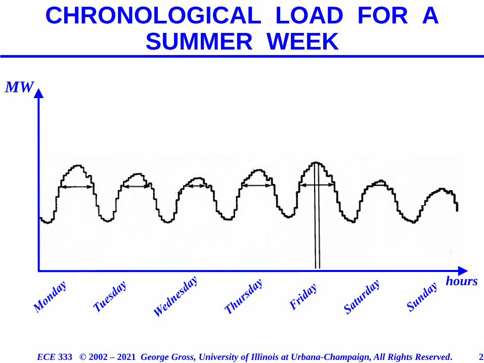
CHRONOLOGICAL LOAD FOR A SUMMER WEEK
MW
hours
ECE 333 © 2002 – 2021 George Gross, University of Illinois at Urbana-Champaign, All Rights Reserved. 3
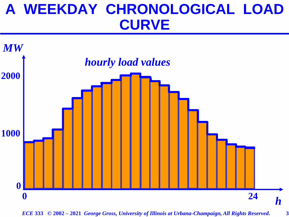
A WEEKDAY CHRONOLOGICAL LOAD CURVE
hourly load values
MW
2000
0
1000
0 24h
ECE 333 © 2002 – 2021 George Gross, University of Illinois at Urbana-Champaign, All Rights Reserved. 4
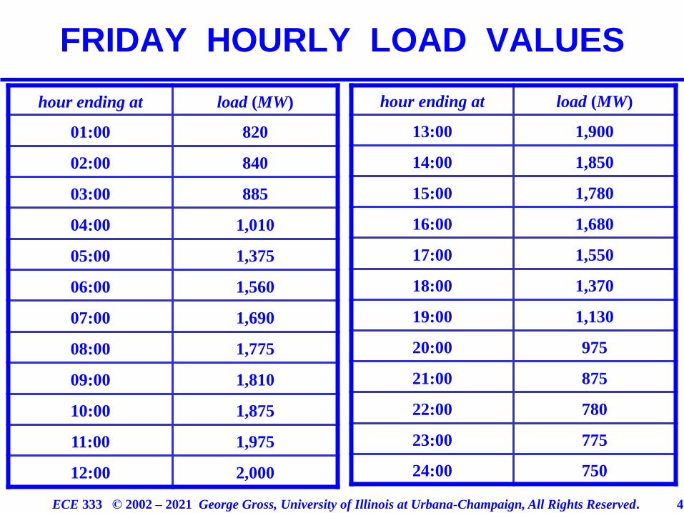
FRIDAY HOURLY LOAD VALUES
hour ending at load (MW)
01:00 820
02:00 840
03:00 885
04:00 1,010
05:00 1,375
06:00 1,560
07:00 1,690
08:00 1,775
09:00 1,810
10:00 1,875
11:00 1,975
12:00 2,000
hour ending at load (MW)
13:00 1,900
14:00 1,850
15:00 1,780
16:00 1,680
17:00 1,550
18:00 1,370
19:00 1,130
20:00 975
21:00 875
22:00 780
23:00 775
24:00 750
ECE 333 © 2002 – 2021 George Gross, University of Illinois at Urbana-Champaign, All Rights Reserved. 5
FRIDAY LOAD DURATION CURVE
hours
MW
2000
0
1000
h
ECE 333 © 2002 – 2021 George Gross, University of Illinois at Urbana-Champaign, All Rights Reserved. 6
CHRONOLOGICAL LOAD FOR A SUMMER WEEK
MW
hours
ECE 333 © 2002 – 2021 George Gross, University of Illinois at Urbana-Champaign, All Rights Reserved. 7
LOAD DURATION CURVE FOR A SUMMER WEEK
MW
1
38.71
168
100 %0
hours65
ECE 333 © 2002 – 2021 George Gross, University of Illinois at Urbana-Champaign, All Rights Reserved. 8
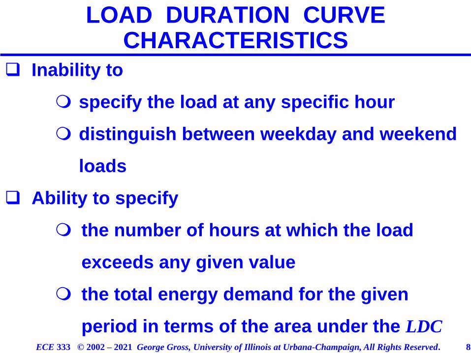
❑ Inability to
specify the load at any specific hour
distinguish between weekday and weekend
loads
❑ Ability to specify
the number of hours at which the load
exceeds any given value
the total energy demand for the given
period in terms of the area under the LDC
LOAD DURATION CURVE CHARACTERISTICS
ECE 333 © 2002 – 2021 George Gross, University of Illinois at Urbana-Champaign, All Rights Reserved. 9
❑ The costs of generation by a conventional unit
are described by a so-called input–output curve,
which specifies the amount of input required to
obtain a specified level of output
❑ Typically, such curves are obtained from actual
measurements and are characterized by their
monotonically non–decreasing forms
CONVENTIONAL GENERATION UNIT ECONOMICS
ECE 333 © 2002 – 2021 George Gross, University of Illinois at Urbana-Champaign, All Rights Reserved. 10
heat input
(MMBtu/h )
output
(MWh/h )
set control valve
points
heat content &
flow–rate of fuel
energy
output
measurement measurement
INPUT – OUTPUT MEASUREMENTS
ECE 333 © 2002 – 2021 George Gross, University of Illinois at Urbana-Champaign, All Rights Reserved. 11
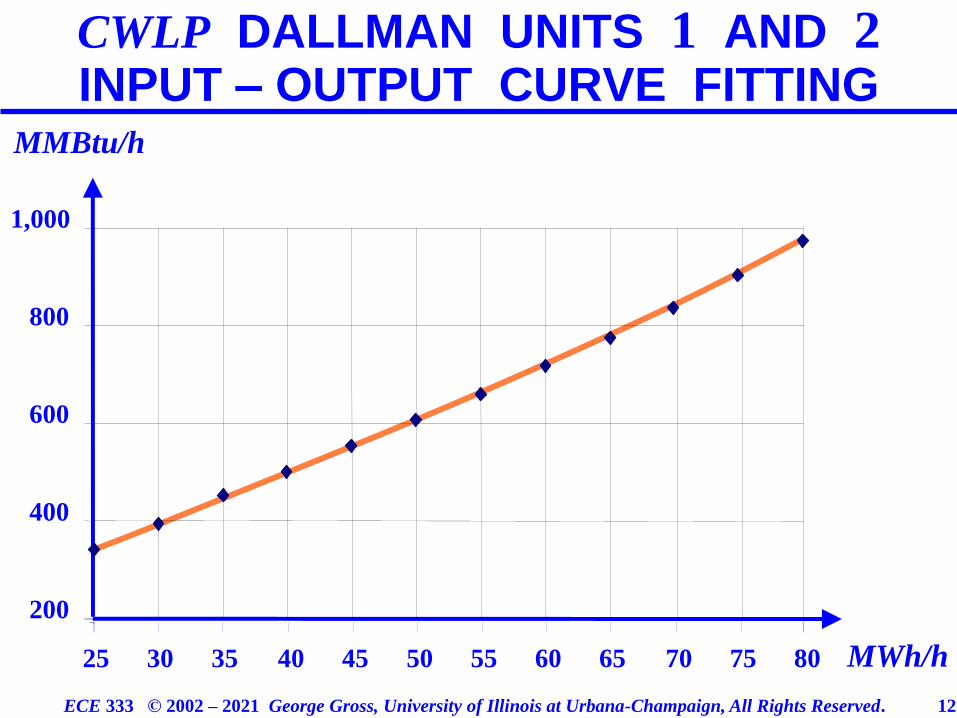
972
901
835
773
715
659
605
552
499
446
392
336
80
75
70
65
60
55
50
45
40
35
30
25
hea
t in
pu
t(
MM
Btu
/h )
ou
tpu
t(
MW
h/h
)
EXAMPLE : CWLP DALLMAN UNITS 1 AND 2
ECE 333 © 2002 – 2021 George Gross, University of Illinois at Urbana-Champaign, All Rights Reserved. 12
CWLP DALLMAN UNITS 1 AND 2INPUT – OUTPUT CURVE FITTING
MMBtu/h
MWh/h
200
400
600
800
1,000
25 30 35 40 45 50 55 60 65 70 75 80
ECE 333 © 2002 – 2021 George Gross, University of Illinois at Urbana-Champaign, All Rights Reserved. 13
❑ The output is in MW and the input is in bbl/h or
Btu/h (volume or thermal heat contents flow rate of
the input fuel)
❑ We may also think of the abscissa in units $/h
since the costs of the input are obtained via a
linear scaling the fuel input by the unit fuel price
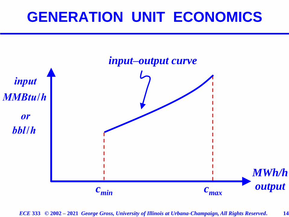
❑ We use the input–output curve to obtain the
incremental input–output curve to determine the costs
to generate an additional MWh at a specified level
of output
GENERATION UNIT ECONOMICS
ECE 333 © 2002 – 2021 George Gross, University of Illinois at Urbana-Champaign, All Rights Reserved. 14
GENERATION UNIT ECONOMICS
MWh/h
output
input
MMBtu/h
or
bbl /h
input–output curve
cmin cmax
ECE 333 © 2002 – 2021 George Gross, University of Illinois at Urbana-Champaign, All Rights Reserved. 15
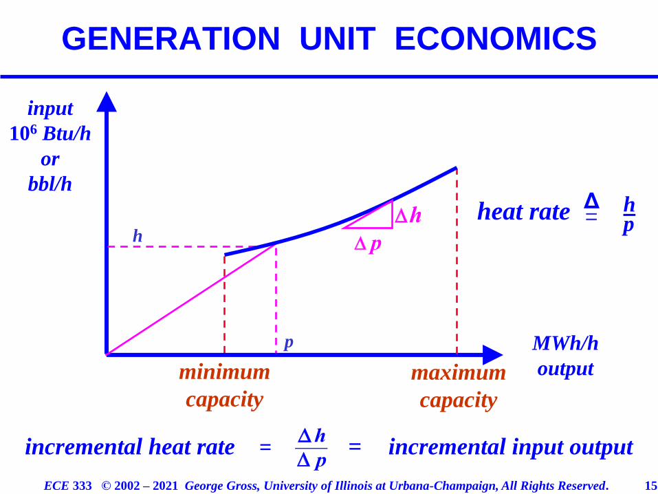
GENERATION UNIT ECONOMICS
incremental heat rate = = incremental input output
heat rate hp=
Δ
h
p
input
106 Btu/h
or
bbl/h
MWh/h
outputminimum
capacity
maximum
capacity
ECE 333 © 2002 – 2021 George Gross, University of Illinois at Urbana-Champaign, All Rights Reserved. 16
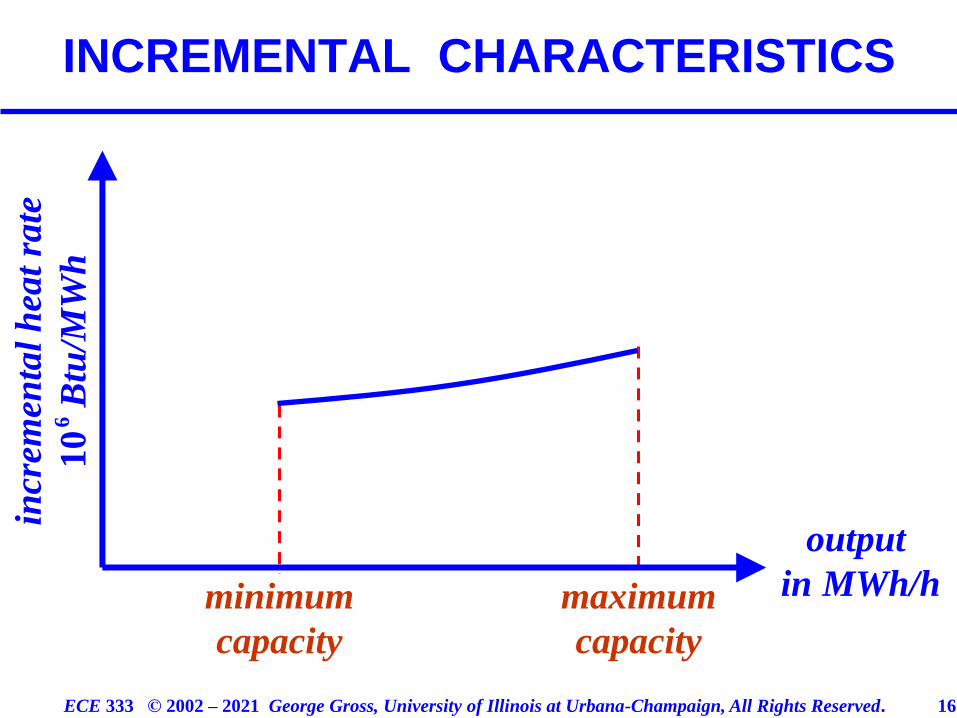
INCREMENTAL CHARACTERISTICS
output
in MWh/hminimum
capacity
maximum
capacity
incr
emen
tal
hea
t ra
te
10
6B
tu/M
Wh
ECE 333 © 2002 – 2021 George Gross, University of Illinois at Urbana-Champaign, All Rights Reserved. 17
HEAT RATE
a possible
operating point
output
MWh/hminimum
capacity
maximum
capacity
heat rate =input
output
incremental
heat rate
=incremental input
incremental output
input
MMBtu/h
ECE 333 © 2002 – 2021 George Gross, University of Illinois at Urbana-Champaign, All Rights Reserved. 18
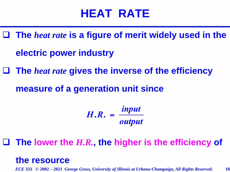
❑ The heat rate is a figure of merit widely used in the
electric power industry
❑ The heat rate gives the inverse of the efficiency
measure of a generation unit since
❑ The lower the H.R., the higher is the efficiency of
the resource
HEAT RATE
ECE 333 © 2002 – 2021 George Gross, University of Illinois at Urbana-Champaign, All Rights Reserved. 19
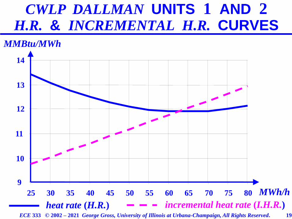
CWLP DALLMAN UNITS 1 AND 2H.R. & INCREMENTAL H.R. CURVES
heat rate (H.R.) incremental heat rate (I.H.R.)
MMBtu/MWh
9
10
11
12
13
14
25 30 35 40 45 50 55 60 65 70 75 80 MWh/h
ECE 333 © 2002 – 2021 George Gross, University of Illinois at Urbana-Champaign, All Rights Reserved. 20
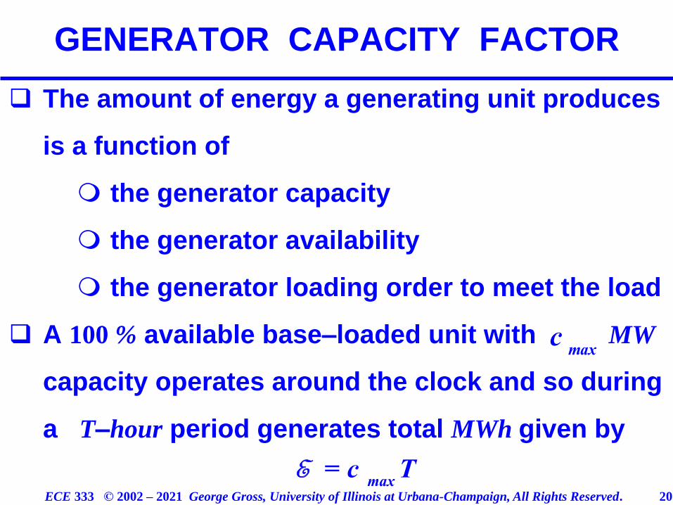
❑ The amount of energy a generating unit produces
is a function of
the generator capacity
the generator availability
the generator loading order to meet the load
❑ A 100 % available base–loaded unit with MW
capacity operates around the clock and so during
a T–hour period generates total MWh given by
GENERATOR CAPACITY FACTOR
cmax
ECE 333 © 2002 – 2021 George Gross, University of Illinois at Urbana-Champaign, All Rights Reserved. 21
❑ The maximum unit can generate over T hours is
❑ The capacity factor of a base-loaded unit is
❑ A cycling unit exhibits on – off behavior since its
loading depends on the system demand; its
exceeds the actual generation since
the unit generates only during certain periods
GENERATOR CAPACITY FACTOR
ECE 333 © 2002 – 2021 George Gross, University of Illinois at Urbana-Champaign, All Rights Reserved. 22
❑ Therefore, a cycling unit has a c.f.
❑ For example, a cycling unit of 150MW that
operates typically 1,800 hours per year with no
outages and at full capacity has
❑ A peaking unit operates only for a few hours each
year and consequently has a relatively low c.f.
GENERATOR CAPACITY FACTOR
ECE 333 © 2002 – 2021 George Gross, University of Illinois at Urbana-Champaign, All Rights Reserved. 23
❑ An expensive peaker may have, say, a c.f.
indicating that under perfect availability it ope-
rates about 438 hours a year
❑ Typically, is defined on an annual basis
where, the denominator may account for annual
maintenance and so the implication is less than
8,760 hours of operation
GENERATOR CAPACITY FACTOR
ECE 333 © 2002 – 2021 George Gross, University of Illinois at Urbana-Champaign, All Rights Reserved. 24
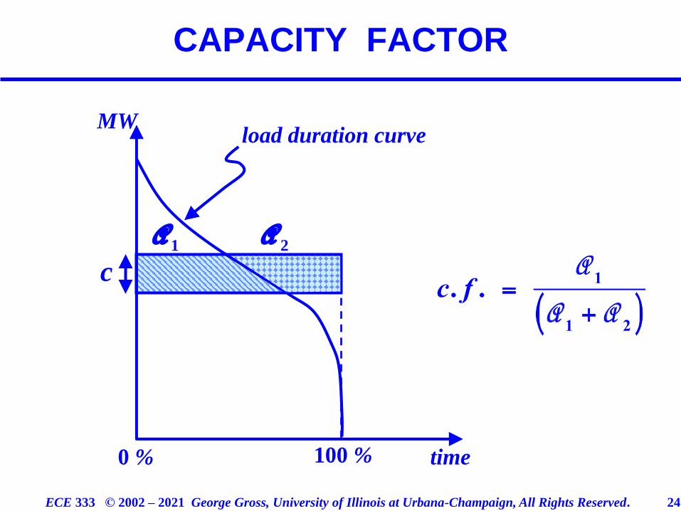
CAPACITY FACTOR
2A
1A
c
MW
time0 % 100 %
load duration curve
ECE 333 © 2002 – 2021 George Gross, University of Illinois at Urbana-Champaign, All Rights Reserved. 25
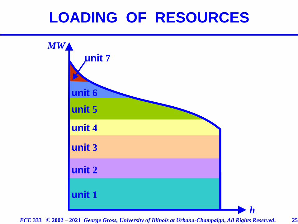
LOADING OF RESOURCES
unit 1
unit 2
unit 3
unit 4
unit 5
unit 6
unit 7
h
MW
ECE 333 © 2002 – 2021 George Gross, University of Illinois at Urbana-Champaign, All Rights Reserved. 26
LOADING OF RESOURCES
Monday Tuesday Wednesday Thursday Friday Saturday Sunday
total available capacity
load
inte
rmed
iate
load
base load
pea
k l
oad
ECE 333 © 2002 – 2021 George Gross, University of Illinois at Urbana-Champaign, All Rights Reserved. 27
❑ Fixed costs are those cost elements that are
independent of the operation of a resource and
are incurred even if the resource is not operating
❑ Typical components of fixed costs are:
investment or capital costs
insurance
fixed O&M
taxes
RESOURCE FIXED AND VARIABLE COSTS
ECE 333 © 2002 – 2021 George Gross, University of Illinois at Urbana-Champaign, All Rights Reserved. 28
❑ Variable costs are associated with the actual
operation of a resource
❑ Key components of variable costs are
fuel costs
variable O&M
emission costs
RESOURCE FIXED AND VARIABLE COSTS
ECE 333 © 2002 – 2021 George Gross, University of Illinois at Urbana-Champaign, All Rights Reserved. 29
❑ The fixed charge rate annualizes the capital costs to
produce a yearly uniform cash–flow set over the
life of a resource
❑ The annual fixed costs are
❑ Typically, the yearly charge is given on a per unit
– kW or MW – basis
ANNUALIZED INVESTMENT OR CAPITAL COSTS
ECE 333 © 2002 – 2021 George Gross, University of Illinois at Urbana-Champaign, All Rights Reserved. 30
❑ The fixed charge rate represents the interest on
loans, acceptable returns for investors and other
fixed cost components: however, each component
is independent of the generated MWh
❑ The rate primarily depends on the costs of capital
ANNUALIZED INVESTMENT OR CAPITAL COSTS
ECE 333 © 2002 – 2021 George Gross, University of Illinois at Urbana-Champaign, All Rights Reserved. 31
❑ The variable costs are a function of the number
of hours of operation of the unit or equivalently
of the capacity factor
❑ The annualized variable costs may vary from
year to year
ANNUALIZED VARIABLE COSTS
ECE 333 © 2002 – 2021 George Gross, University of Illinois at Urbana-Champaign, All Rights Reserved. 32
❑ The yearly variable costs explicitly account for
fuel cost escalation
❑ Often, the yearly costs are given on a per unit – kW
or MW – basis
❑ We illustrate these concepts with a pulverized –
coal steam plant
ANNUALIZED VARIABLE COSTS
ECE 333 © 2002 – 2021 George Gross, University of Illinois at Urbana-Champaign, All Rights Reserved. 33
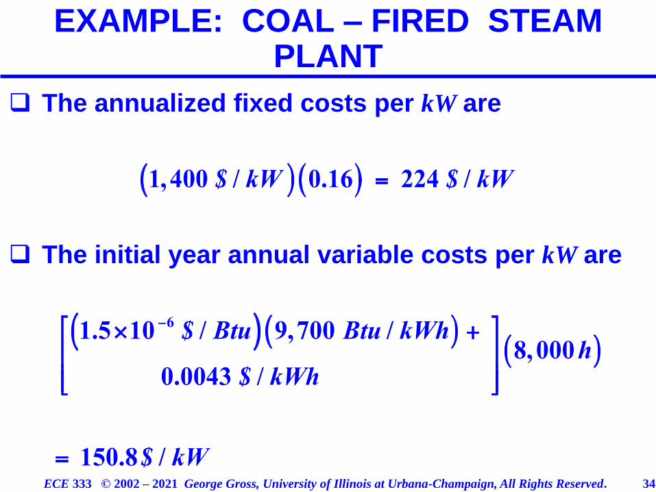
EXAMPLE: COAL – FIRED STEAM PLANT
characteristic value unit
capital costs 1,400 $/kW
heat rate 9,700 Btu/kWh
fuel costs 1.5 $/MBtu
variable costs 0.0043 $/kWh
annual fixed charge rate 0.16 –––
full output period 8,000 h
ECE 333 © 2002 – 2021 George Gross, University of Illinois at Urbana-Champaign, All Rights Reserved. 34
❑ The annualized fixed costs per kW are
❑ The initial year annual variable costs per kW are
EXAMPLE: COAL – FIRED STEAM PLANT
ECE 333 © 2002 – 2021 George Gross, University of Illinois at Urbana-Champaign, All Rights Reserved. 35
❑ Total annual costs for 8,000 h are
❑ Note, we do the example under the assumption of
full output for 8,000 h and 0 output for the
remaining 760 h of the year
❑ We also neglect any possible outages of the unit
and so explicitly ignore any uncertainty in the
unit performance
EXAMPLE: COAL – FIRED STEAM PLANT
ECE 333 © 2002 – 2021 George Gross, University of Illinois at Urbana-Champaign, All Rights Reserved. 36
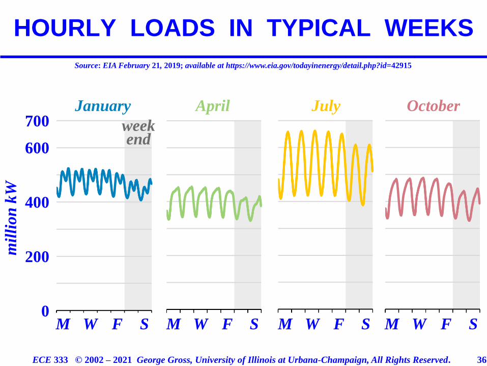
HOURLY LOADS IN TYPICAL WEEKS
Source: EIA February 21, 2019; available at https://www.eia.gov/todayinenergy/detail.php?id=42915
mil
lion
kW
0
200
400
600
700
M W F S M W F S M W F S M W F S
January April July October
week end
ECE 333 © 2002 – 2021 George Gross, University of Illinois at Urbana-Champaign, All Rights Reserved. 37
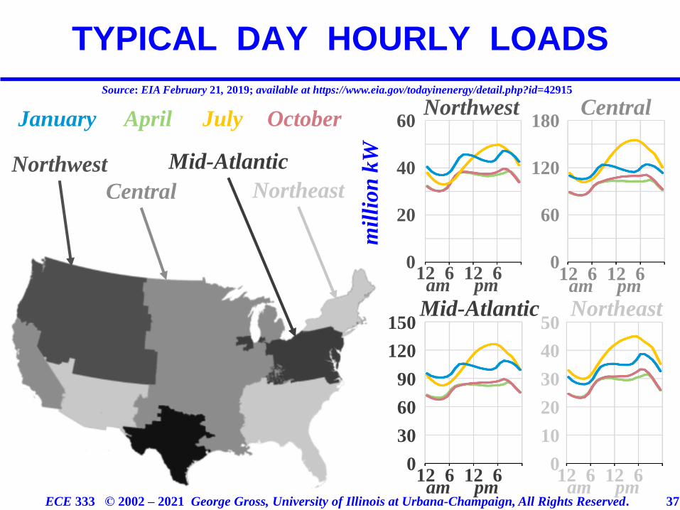
TYPICAL DAY HOURLY LOADS
Source: EIA February 21, 2019; available at https://www.eia.gov/todayinenergy/detail.php?id=42915
mil
lion
kW
Northwest Central
NortheastMid-Atlantic
0
20
40
60
12am pm
6 6120
60
120
180
0
10
30
50
40
20
0
30
90
150
120
60
12am pm
6 612 12am pm
6 612
12am pm
6 612
January April July October
Northwest
Central Northeast
Mid-Atlantic
ECE 333 © 2002 – 2021 George Gross, University of Illinois at Urbana-Champaign, All Rights Reserved. 38
mil
lon
kW
California Southwest
SoutheastTexas
0
20
40
60
12am pm
6 6120
5
15
25
0
30
180
120
0
15
45
75
60
30
12am pm
6 612 12am pm
6 612
12am pm
6 612
January April July October
20
10
California
Southwest Southeast
Texas
Source: EIA February 21, 2019; available at https://www.eia.gov/todayinenergy/detail.php?id=42915
TYPICAL DAY HOURLY LOADS