9. Comp Sci - IJCSE - PID Control Strategy in Networked Control System - Anshu Mala Kispotta (1)

www.iaset.us [email protected]

PID CONTROL STRATEGY IN NETWORKED CONTROL SYSTEM

ANS HU MALA KISPOTTA

M.Tech (EE-Control System), BIT Sindri, Dhanbad, Jharkhand, India

ABSTRACT

The networked control systems (NCS) and sensor networks, where the process , actuator and the controller are

separated by a network, are d iscussed in this paper and new problems in control are pointed out. To overcome new

controller tuning techniques are needed. In this paper Discrete-time PID controller tuning for varying time-delay systems,

including NCS are discussed. Optimal PID tuning results are presented for a general process model in different cases of

constant, state- and time-dependent or random delays. The results are displayed as functions of process time constant and

controller sampling time. PID controller design methods such as internal model control and gain scheduling are discussed

in this thesis and also we develop and compare the data fusion methods in NCS.

KEYWORDS: Networked Control Systems, Discrete-Time PID Controller, Tuning, Vary ing Time-Delay

1. INTRODUCTION

Networked control systems (NCS) are feedback control systems wherein the control loops are closed through a

real-t ime network. The main motivations for using networks for data transmissions in control systems are reduced system

wiring, ease of system diagnosis. The problem is that the network induces a varying time -delay into the control loop, which

has to be taken into account in control design. Conventional control design can’t take the varying time-delay into account,

new methods are called upon. Networked control systems (NCS) are researched and some results have been achieved.

Dynamic programming has been proposed for controlling varying time-delay systems. But still simple tuning rules for

varying time-delay systems are needed. The thesis investigates optimization in tuning controllers for varying time-delay

systems using simulat ion.

A PID controller structure is selected to control the system as it is easy and intuitive to tune. It is used in industrial

controller and also has on a particular fixed structure controller family, so it is called PID controller family. PID controllers

are commonly used in industry and a large factory may have thousands of them, in instru ments and laboratory equipment.

In engineering applications the controllers appear in many d ifferent forms: as a standalone controller, as part of

hierarchical, d istributed control systems, or built into embedded components. The simplicity of these controllers is also

their weakness - it limits the range of plants that they can control satisfactory.

In modern industry where discrete time PID controllers are used the controllers are tuned as if they where

continuous controllers. The sampling frequency is set sufficiently high, so that the discrete-time controller approximates a

continuous controller. This is possible if there is enough computing power and signaling capacity. In some new

applications these are not always available. In networked control systems the network can’t offer high bandwidth to

transmit the measurement and control packets. The energy source and the computing power are often limited on mobile

devices, such as robots and autonomous devices. In these applications one has to enter the true discrete -time domain by

lowering the sample frequency.

International Journal of Computer Science and Engineering (IJCSE) ISSN(P): 2278-9960; ISSN(E): 2278-9979 Vol. 3, Issue 3, May 2014, 67-82

© IASET

http://www.iaset.us/

68 Anshu Mala Kispotta

Impact Factor (JCC): 3.1323 Index Copernicus Value (ICV): 3.0

The main contributions of this thesis are:

Modification of the optimization and simulation based tuning method for discrete-time PID controllers in NCS.

Tuning rules for a first order system with several vary ing delays.

Internal model control and gain scheduling

Development and comparison of data fusion methods in NCS.

The results, methods and the theory they are based on, are presented in the paper as follows: First varying

time-delay systems are generally introduced and the time-delays in these systems are identified and analyzed, including the

delay distribution of the Internet. Then networked control systems are explained in section 2. The discrete time PID

controller and the optimizat ion tuning are presented in section 3 among with other PID controller design methods such as

internal model control and gain scheduling. The optimization tuning method is applied in a general case for a first order

system and for a certain example process in section 4.

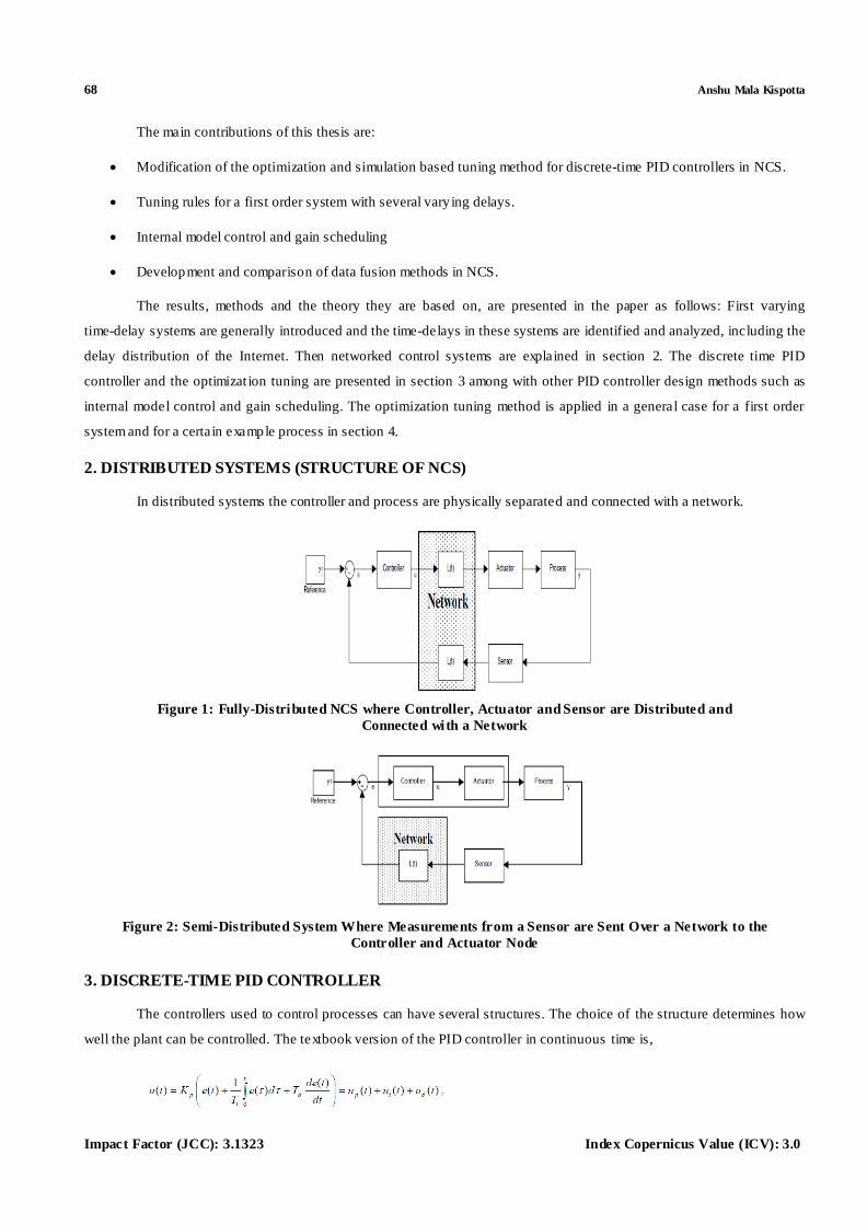
2. DISTRIBUTED SYSTEMS (STRUCTURE OF NCS)

In distributed systems the controller and process are physically separated and connected with a network.

Figure 1: Fully-Distributed NCS where Controller, Actuator and Sensor are Distributed and

Connected with a Network

Figure 2: Semi-Distributed System Where Measurements from a Sensor are Sent Over a Network to the

Controller and Actuator Node

3. DISCRETE-TIME PID CONTROLLER

The controllers used to control processes can have several structures. The choice of the structure determines how

well the plant can be controlled. The textbook version of the PID controller in continuous time is,

PID Control Strategy in Networked Control System 69


Where e (t) is,

The reference signal (the set-point) is yr(t) and the output is y(t) of the controlled process, with L(t ) = 0.

In transfer function above Equation becomes

The coefficients Kp, Ti, Td and P, I, D are related by:

The proportional part of the controller at time -step k is then

The integral part is

Discretised by approximating the integral with a sum

This can further be simplified by computing the difference

The derivative part, ud[k] is,

Which is usually not used since it amplifies random errors.




4. OPTIMIZATION FOR DIFFERENT DELAYS

The total ITAE cost is thus,

The process is a simple first order system with time constant T and transfer function

The process is augmented with a varying time delay, L (t),

Figure 3: Model of a System with Varying Time-Delay

The delay can be a) constant, b) random, c) time-dependent, d) state- dependent. The respective delays used in

these cases are described by,

τ (t) = L

τ (t) = rand[0.8...1.2] (6.3)

τ (t) = sin(t )

τ (t) = x(t )

4.1.1 Case 1a-Constant Delay- First, the PID controller is optimized for a constant delay in the process.

Figure 4: Optimal PID Controller Parameters for the First Order System with Constant Delay. P, I, D and Cost as Functions of Process Time Constant, T and Controller Sampling Time, h



4.1.2 Case 1b - Random Delay

Figure 5: Optimal PID Controller Parameters for the First Order System with Random Delay

P, I, D and Cost as Functions of Process Time Constant, T and Controller Sampling Time, h

Comparing the result shown in Figure 5 and the previous result there are only slight differences. The P and I terms

are practically identical. There is some arbitrariness in the controller parameters, especially in the D term. This is caused by

the randomness in the delay. As the results are similar to the constant case, one can assume a constant delay

(the mean of the random) when tuning a PID controller for this kind of uniformly distributed random delay.

4.1.3 Case 1c - Sinusoidal Delay

In this case the time-delay varies like a sinusoid. The results are shown in Figure 6.

Figure 6: Optimal PID Controller Parameters for the First Order System with Sinusoidal Delay

P, I, D and Cost as Functions of Process Time Constant, T and Controller Sampling Time , h

4.1.4 Case 1d - State Delay

The same system is now optimized with a state-dependent delay.




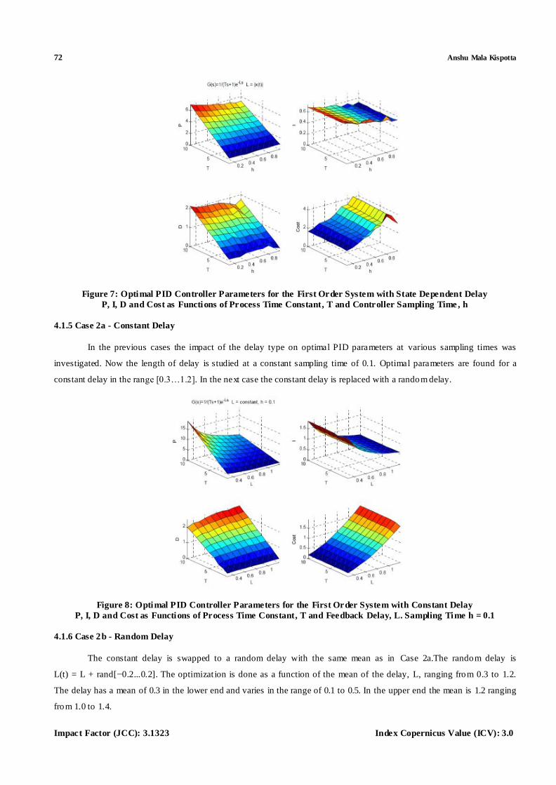
Figure 7: Optimal PID Controller Parameters for the First Order System with State Dependent Delay

P, I, D and Cost as Functions of Process Time Constant, T and Controller Sampling Time , h

4.1.5 Case 2a - Constant Delay

In the previous cases the impact of the delay type on optimal PID parameters at various sampling times was

investigated. Now the length of delay is studied at a constant sampling time of 0.1. Optimal parameters are found for a

constant delay in the range [0.3…1.2]. In the next case the constant delay is replaced with a random delay.

Figure 8: Optimal PID Controller Parameters for the First Order System with Constant Delay

P, I, D and Cost as Functions of Process Time Constant, T and Feedback Delay, L. Sampling Time h = 0.1

4.1.6 Case 2b - Random Delay

The constant delay is swapped to a random delay with the same mean as in Case 2a.The random delay is

L(t) = L + rand[−0.2...0.2]. The optimizat ion is done as a function of the mean of the delay, L, ranging from 0.3 to 1.2.

The delay has a mean of 0.3 in the lower end and varies in the range of 0.1 to 0.5. In the upper end the mean is 1.2 ranging

from 1.0 to 1.4.



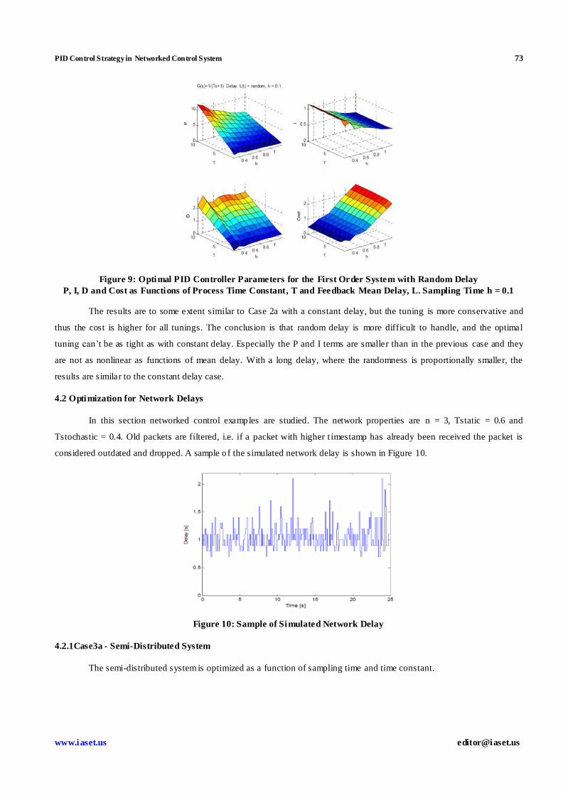
Figure 9: Optimal PID Controller Parameters for the First Order System with Random Delay

P, I, D and Cost as Functions of Process Time Constant, T and Feedback Mean Delay, L. Sampling Time h = 0.1

The results are to some extent similar to Case 2a with a constant delay, but the tuning is more conservative and

thus the cost is higher for all tunings. The conclusion is that random delay is more difficult to handle, and the optimal

tuning can’t be as tight as with constant delay. Especially the P and I terms are smaller than in the previous case and they

are not as nonlinear as functions of mean delay. With a long delay, where the randomness is proportionally smaller, the

results are similar to the constant delay case.

4.2 Optimization for Network Delays

In this section networked control examples are studied. The network properties are n = 3, Tstatic = 0.6 and

Tstochastic = 0.4. Old packets are filtered, i.e. if a packet with higher t imestamp has already been received the packet is

considered outdated and dropped. A sample o f the simulated network delay is shown in Figure 10.

Figure 10: Sample of Simulated Network Delay

4.2.1Case3a - Semi-Distributed System

The semi-distributed system is optimized as a function of sampling time and time constant.




Figure 11: Optimal PID Controller Parameters for the First Order, Semi-Distributed System with Network Delay

P, I, D and Cost as Functions of Process Time Constant, T, and Controller Sampling Time, h

Comparing this and Case 1b (random delay) the results are to some degree similar.

The P, I and D terms are almost the same. The cost is smaller because the error signal is not taken after the delay,

but right from the process output. The cost is, though in another manner, increasing with sampling time, with dips as the

delay turns into constant at the larger sample t imes.

4.2.2Case3b- Fully-Distributed System

The system in the previous case is extended to a fully-distributed system. Now there is an additional delay

between the controller and the process. This leads not only to a larger delay in the control loop, but also to a higher cost, as

the delay is between the reference signal and the process output signal.

Figure 12: Optimal PID Controller Parameters for the First Order, Fully-Distributed System with Network Delay P, I, D and Cost as Functions of Process Time Constant, T and Controller Sampling Time, h

4.3 Gain Scheduling by Delay

In this case the gain scheduling is based on the current average delay of the system, in practice on a low-pass

filtered measured delay. The gain scheduling strategy investigated here is depicted in Figure 13.



Figure 13: Gain Scheduling with PID Controller. The Gain Scheduler has a Low-Pass

Filter for the Delay and Look-up Tables for P, I and D Parameters

First the delay is random with the same properties as in Case 2b, but there is a step in the mean delay from 0.5 to

1.0 at time 40 s. In the second example the delay has a slow sinusoidal variation with a frequency of 0.1 rad/s and

amplitude 0.4.

Figure 14: Delay for Simulations with Gain Scheduling. Thin Line: Measured Delay, Bold Line: Low-Pass

Filtered Delay on the Left: Random Delay with Step Change. On the Right: Slow Sinusoidal Variation

4.3.1 Case 4a – Step Delay Change

The nominal delay of the system is assumed to be 0.5. The constant controller is tuned for this delay. At some

stage the state of the system changes and the delay rises to 1.0. Examination of the step responses on the right in

Figure 15 leads to the conclusion that the gain scheduled controller is better than the non-scheduled controller The PID

parameters plotted in on the left show that, indeed, the controller is scheduled with appropriate gains for the current delay.

Figure 15: Gain Scheduling with Step Delay Change. On the Left: PID Parameters for Current Identified

Delay as Function of Time. On the Right: Step Res ponses for System with and without Gain Scheduling




4.3.2 Case 4b – Sinusoidal Delay Change

In this case the random delay is assumed to have slow sinusoidal variations with amplitude 0.4 around a mean

delay of 0.75. For the sinusoidal delay the controller tuned for an average variat ion does perform well sometimes, but as

the delay changes the control loop has overshoots and there is risk of instability. These two cases show that a gain

scheduled PID controller performs better than a constant controller, when the delay changes significantly.

Figure 16: Gain Scheduling with Sinusoidal Delay Change. On the Left: PID Parameters as

Functions of Time on the Right: Step Res ponses of the System with and without Gain Scheduling

4.4 Sensor Network

A sensor network is considered here with the sensor cluster having four sensors with known noise variances.

The controller is hand tuned (P = 1, I = 0.7 and D = 0.2, this is near the optimal tuning for the system) to get a satisfactory

step response. The simulation is run for four step responses, and the error integrals are averaged to get a better estimat ion

of them, because of the randomness (noise, delay, packet loss) in the network that causes varying performance on the step

responses at different times. The strategies are evaluated based on their step response ITAE and the fusion error IAE over

the whole simulat ion. The results are shown in the following figures and collected in Tab le 1.

Table1: Fusion Strategies Results

case Name Step Res ponse

ITAE

Fusion

Error IAE

1 Fusion_no 1.56 3.7

2 Fusion 1.36 1.33

3 Fusion_by_timestamp 1.16 1.12

4 Fusion_by_timestamp2 1.85 3.05

5 Fusion_with_delay 1.21 1.61

Figure 17: Simulated Step Responses (Top) and Control Signals (Bottom) with Various Fusion Strategies



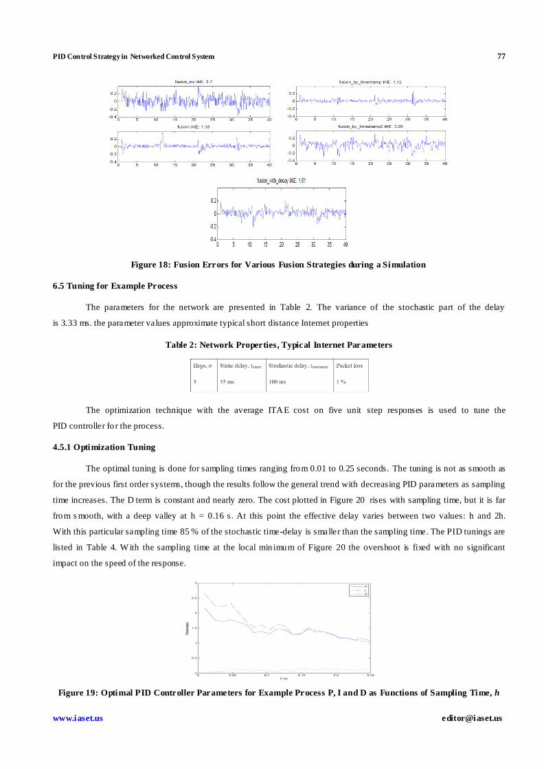
Figure 18: Fusion Errors for Various Fusion Strategies during a Simulation

6.5 Tuning for Example Process

The parameters for the network are presented in Table 2. The variance of the stochastic part of the delay

is 3.33 ms. the parameter values approximate typical short distance Internet properties

Table 2: Network Properties, Typical Internet Parameters

The optimization technique with the average ITAE cost on five unit step responses is used to tune the

PID controller fo r the process.

4.5.1 Optimization Tuning

The optimal tuning is done for sampling times ranging from 0.01 to 0.25 seconds. The tuning is not as smooth as

for the previous first order systems, though the results follow the general trend with decreasing PID parameters as sampling

time increases. The D term is constant and nearly zero. The cost plotted in Figure 20 rises with sampling time, but it is far

from s mooth, with a deep valley at h = 0.16 s. At this point the effective delay varies between two values: h and 2h.

With this particular sampling time 85 % of the stochastic time-delay is smaller than the sampling time. The PID tunings are

listed in Table 4. W ith the sampling time at the local min imum of Figure 20 the overshoot is fixed with no significant

impact on the speed of the response.

Figure 19: Optimal PID Controller Parameters for Example Process P, I and D as Functions of Sampling Time, h




Figure 20: Optimal ITAE Cost as a Function of Sampling Time, h, for Example Process

Figure 21: Step Res ponses with Optimization Tuning. Sampling Times: 0.025, 0.16 and 0.25 Seconds

4.5.2 Ziegler-Nichols Tuning

To compare the results of the optimization based tuning, other tuning methods are also tested. With the simulation

model both Ziegler-Nichols step- and frequency response tuning is made. The step response and the critical gain tests are

shown in Figure 22.

Figure 22: Step Res ponse (left) and Frequency Response Tests for Ziegler-Nichols Tuning

From these graphs the required properties are measured and the parameters are calculated according to Table 1 and

translated to P, I and D parameters using Equation I=Kp/Ti. The relevant measurements are collected in Tab le 3.

Table 3

Ku Tu T1 T2

Simulation 4.5 0.97 0.25 0.7

Test Run 4.5 1.1 0.22 0.8

The Z-N tuning does not take into account the sampling time. A low sampling time is used h = 0.025 s, where the

controller approximates a continuous-time controller to some degree. For higher sampling times the control loop becomes

unstable.



4.5.3 IMC Tuning

The IMC 63 concept ensures that the controller will work and compensate for the (artificial) modeling error.

The controller is tested with and without the pre-filter. The parameters in Equation Td=a2/a1 are derived in the

continuous-time case because an IMC controller derived in d iscrete-time can’t be brought to a PID controller form.

Therefore only a short sampling time of h = 0.025 s is used for the discrete-time PID so that it approximates the

continuous-time controller. The tuning parameter, λ, for the IMC tuning is selected to be 0.65.This results in a response

with litt le overshoot, and with minimum ITAE cost are shown in figure 23.

Figure 23: IMC Tuning with Pre-Filter. Simulated Step Responses for the Example Process

4.5.4 RESULTS

The process responses and the control signals for a series of reference step changes are displayed in the following

figures. The PID parameters obtained with the different tuning methods and the respective average ITAE and IAE costs of

the step responses. The ITAE costs of the responses are used to compare the tuning methods. This measure is chosen

because it takes the whole response into account, which is not the case for measures such as the rise time or overshoot.

The Z-N step response method is almost unstable and oscillates heavily: the cost is 6 times larger compared to the optimal

tuning. This is due to the large gains of the tuning. The Z-N tuning methods are designed for load disturbance rejection so

the poor performances originate partially from the reference step changes in the simulat ions. The IMC tuning with a

pre-filter has a quite different step response compared to the others and does not belong here because of the filtering in

addition to the pure PID controller. The optimization method has the lowest ITAE and IAE cost, followed by IMC.

There is a correlation between the ITAE and IAE costs. The square integral costs (ISE and ITSE, not shown) give similar

results.

Table 4: PID Parameters for Example Process and Cost from Simulations

Method P I D Cost ITAE Cost IAE

Z-N step response 3.36 6.72 0.42 0.072 0.302

Z-N frequency response 2.7 5.57 0.33 0.027 0.034

Optimization,h=0.025 1.77 2.66 0.02 0.014 0.021

Optimization, h=0.16 1.48 1.50 0.13 0.015 0.024

Optimization, h=0.025 1.08 1.05 0.11 0.025 0.051

IMC(without pre-filter) 1.56 1.23 0.25 0.025 0.022

IMC(with pre-filter) 1.56 1.23 0.25 0.026 0.046

The tuning by optimization is the best, it has the smoothest response and settles down in a short time with little

overshoot, even the larger step is not a problem. The tuning for a sampling t ime of h = 0.25 s works almost as well, there is

only a larger delay and a slower response because of the large sampling time. It is notable that the IMC tuning




(with and without a pre-filter) comes near the same performance as the optimal tuning, if one considers the error integrals.

The control signals shows that the Z-N and the IMC tuning are aggressive with large control signals. The Z-N tuning

oscillates strongly. The optimal tunings have a reliable and precise control signal in comparison to the other methods.

Figure 24: Simulated Step Responses for Example Process

Figure 25: Control Signals for Example Process

8 CONCLUSIONS

This paper studied that the discrete-time PID controller designs and tuning for varying time-delay systems and

furthermore networked control systems (NCS), including sensor networks. The discrete-time PID controller was introduced

and some practical aspects, such as derivative filtering were fo rmulated. As NCS includes a network, which transmits

measurements as packets, there is an inherit discreteness to the system and therefore only discrete-time PID controllers

were studied. The controller tuning was focused on an optimization by simulat ion technique. The tuning method was

modified to work with discrete-time controllers in the context of NCSs. Other PID design methods such as Ziegler-Nichols

and Internal Model Control were compared to the optimization method. It was further shown to perform better than

traditional tuning methods, because it can take the varying time -delay better into account. A general study of optimal

tuning for varying time-delay systems was conducted. The optimizat ion was done for first-order systems with time-delay,

as a function of process time constant and controller sampling time. The t ime-delay was a varying time-delay, namely

time- or state-dependent and random. The results gave rules of thumbs to tune the PID controller for different types of

time-delays. One general result was that with increasing sampling time the P and I terms decrease. With increasing process

time constant the P and D terms increase. The tuning results of different time-varying delays were compared to the

constant delay case. Differences in the optimal tuning with different types of time-delays were 74 found. However, the

optimal tuning for a random delay with a s mall variance is virtually the same as in the constant delay case.

In the case of a small random variance in the time-delay and a larger sampling time, constant delay tuning can be

used, as the sampling time rounds the delay up to nearly constant. The PID controller was found to work best when most of

the stochastic time-delay was smaller than or equal to the sampling time of the controller. It performs equally well with a

short enough sampling time, with the expense of a more active control signal and less robust performance. The optimized



tuning results were based on the ITAE cost of the error signal. As the optimization focused on the time-response only,

robustness is not guaranteed. Robustness, load disturbance rejection and noise rejection can easily be incorporated into the

optimization criteria.

The down-side of the optimization technique is that a process model is needed. The model can, however, be any

input-output description and it is not limited to linear and time-invariant systems. This allows one to tune for any type of

processes, such as processes with time-varying delay which is done in this paper. Networked control systems and their

various layouts, including sensor networks were described. The occurrence of a time-delay in the control loop of these

systems was analyzed. Especially the delay distribution in the Internet was described in detail. Sensor fusion methods for

sensor network systems were developed and tested in the simulat ions. Gain scheduling based on delay was also

demonstrated with typical delay changes corresponding to fall off of a node and daily network utilizat ion changes. The

optimization method was applied on networked control systems, where the varying time-delay was modeled with the

Internet delay distribution. Several tuning methods were tested on an example process in simu lations. The optimizat ion

tuning cost as a function of sampling time showed that there is a local min imum at a relatively long sampling time where

the performance of the controller good. The favorable sampling time is such that the resulting effective delay varies

between two values. It is showed that a PID controller can be used to control a process with varying time-delay, as long as

the variation in the delay is small, in the order of the sampling time. Tradit ional tuning methods, such as Ziegler-Nichols,

do not perform well in the new setting of networked control systems. The tuning can instead be done with the optimizat ion

tuning method using simulation described in it.

ACKNOWLEDGEMENTS

This work has been supported by under the guidance of Mrs. Rekha Jha, Prof. A. Kujur, Mr. Ankush sir and my

sisters Megha and Abha.

REFERENCES

1. Y. Tipsuwan and M. Chow, “Control Methodologies in Networked Control Systems,” Control Engineering

Practice, vol. 11, pp. 1099–1111, 2003.

2. W. Zhang, M. S. Branicky and S. M. Phillips, “Stability of Networked Control Systems,” IEEE Control Systems

Magazine, pp. 84-99, February 2001.

3. H. Lin and P. J. Antsaklis, “Stability and Persistent Disturbance Attenuation Properties for a Class of Networked

Control Systems: Switched System Approach,” International Journal of Control, vol. 78, No. 18, pp. 1447–1458,

2005.

4. Alves, M.Tovar, E.Vasques F. 2000. Ethernet Goes Real-t ime: a Survey on Research and Technological

Developments Hurray-TR-2K01.

5. Bolot, J. C. 1993 Characterizing End-to-End Packet Delay and Loss in the Internet Journal of High-Speed

Networks Sigcomm 1993. pp. 289 – 298.

6. Cao, J. W illiam, S. C. Lin, D. Sun D. 2002. Internet Traffic Tends Toward Poisson and Independent as the Load

Increases Nonlinear Estimation and Classificat ion. Springer Verlag, New York, NY, Dec. 2002.

ISBN: 0-387- 95471-6.




7. Y. Tipsuwan and M.Y. Chow, “Gain Scheduler Middleware: A Methodology to Enable Existing Controllers for

Networked Control and Teleoperation—Part I Networked Control,” IEEE Transactions on Industrial Electronics,

vol. 51, No.6, pp. 1218-1227, 2004.

8. R.M. Miller, S.L. Shah, R.K. Wood and E.K. Kwok, “Predictive PID,” ISA Transactions, vol.38, pp. 11-23, 1999.

9. S. H. Kim and P. Park, “Network-delay-dependent H-ink control of systems with input saturation,” Proc. of the

2007 WSEAS International Conference on Computer Engineering and Applications , Gold Coast, Australia, 2007,

pp. 117-121.

10. Ekanayake, M.M. Premaratne, K., Douligeris, C., Bauer, P.H. 2001.Stability of Discrete-Time Systems with

Time-Varying Delays in proc American Control Conference Arlington VA 2001.

11. Eriksson L2005 A PID Tuning Tool for Networked Control Systems WSEAS Transactions on Systems, Issue1

Vol. 4 ISSN: 1109-2777.

12. Eriksson, L. and Koivo, H. 2005. Tuning of Discrete-Time PID Controllers in Sensor Network based Control

Systems in proc 6th IEEE International Symposiu m on Computational Intelligence in Robotics and Automation

Espoo, Fin land. 2005.

13. Hanselmann, H. 1996. Automotive Control: From Concept to Experiment to Product. In proc. IEEE International

Symposium on Computer-Aided Control System Design. Dearborn, MI, 1996.

14. Garcia, C E and Morari M 1982 Internal Model Control 1 A Unify ing Review and Some New Results Industrial,

Engineering Chemistry Process Design and Development Vol. 21, No 2, 1982.

15. Isaksson, A.J. and Graebe, S.F. 2002. Derivative filter is an integral part of PID design. IEE Proceedings Control

Theory and Applications 61 149, No I January 2002. ISSN: 1350-2379.

16. Katayama, T, McKelvey T, Sano, A, Cassandras C, Camp, M. 2005 Trends in Systems and Signals In proc 16th

IFAC World Congress, Prague, Czech Republic, 2005.

17. Leith, DJ and Leithead, W E 2000 Survey of gain-scheduling analysis and design International Journal of Control,

Vol 73, No 11 2000.

18. Lincoln B 2003 Dynamic p rogramming and Time-Varying Delay Systems PhD thesis Department of Automatic

Control Lund institute of Technology Sweden 2003.

19. Liu G.P., Yang, J.B., Whidborne, J.F. 2003. Mult iobjective Opt imization and Control, Research Studies Press Ltd,

England. ISBN: 0-86380-278-8.

20. Liu, X. and Goldsmith, A. 2004. Kalman filtering with partial observation losses 43rd IEEE Conference on IEEE

Decision and Control Volume: 4, 2004.

21. Nilsson, J. 1998. Real-Time Control Systems with Delays Master’s thesis Department of Automatic Control Lund

Institute of Technology Sweden ISSN 0280–5316.

Date post:	11-May-2017
Category:	Documents
Upload:	suma
View:	216 times
Download:	1 times

9. Comp Sci - IJCSE - PID Control Strategy in Networked Control System - Anshu Mala Kispotta (1)

Documents