9. Functions of several variables These lecture notes present my interpretation of Ruth Lawrence’s lec- ture notes (in Hebrew) 1 9.1 Definition In the previous chapter we studied paths (;&-*2/), which are functions R → R n . We saw a path in R n can be represented by a vector of n real-valued functions. In this chapter we consider functions R n → R, i.e., functions whose input is an ordered set of n numbers and whose output is a single real number. In the next chapter we will generalize both topics and consider functions that take a vector with n components and return a vector with m components. Example 9.1 Consider the function f ∶ R 2 → R defined by f (x, y) = x 2 + y sin x. We may as well write f ∶ (s, t ) s 2 + t sin s, but since the number of arguments can be larger, it is more systematic to use the vector notation, f (x ) = f (x 1 , x 2 ) = x 2 1 + x 2 sin x 1 . 1 Image of Joseph-Louis Lagrange, 1736–1813
Transcript
9. Functions of several variables
These lecture notes present my interpretation of Ruth Lawrence’s lec-ture notes (in Hebrew)1
9.1 Definition
In the previous chapter we studied paths (�;&-*2/), which are functions R→Rn. Wesaw a path in Rn can be represented by a vector of n real-valued functions. In thischapter we consider functions Rn→R, i.e., functions whose input is an ordered setof n numbers and whose output is a single real number. In the next chapter we willgeneralize both topics and consider functions that take a vector with n componentsand return a vector with m components.
� Example 9.1 Consider the function f ∶R2→R defined by
f (x,y) = x2+y sinx.
We may as well writef ∶ (s,t)� s2+ t sins,
but since the number of arguments can be larger, it is more systematic to use thevector notation,
f (x) = f (x1,x2) = x21+x2 sinx1.
�1Image of Joseph-Louis Lagrange, 1736–1813
120 Functions of several variables
� Example 9.2 Like for the case n = 1, the domain of a function may be a subset ofRn. For example, let
D = {(x,y,z) ∈R3 � x2+y2+ z2 < 1} ⊂R3,
or in vector notation,D = {x ∈R3 � �x� < 1} ⊂R3.
Define g ∶D→R by
g(x) = ln(1− �x�2) or g(x,y,z) = ln(1−x2−y2− z2).Then, for example, (1�2,1�2,1�2) ∈D and
g(1�2,1�2,1�2) = ln14.
�Comment 9.1 It is very common to denote the arguments of a bi-variate functionby (x,y) and of a tri-variate function by (x,y,z). We will often do so, but rememberthat there is nothing special about these choices.
� Example 9.3 Important example! Recall that if V and W are vector spaces,we denote by L(V,W) the space of linear functions V →W . Let a ∈Rn. Then thefunction,
f ∶Rn→R defined by f ∶ x� a ⋅xis linear, i.e., belongs to L(Rn,R), in the sense that for every x,y ∈Rn and a,b ∈R,
f (ax+by) = a f (x)+b f (y).For example, taking n = 3 and a = (1,2,3),
f (x,y,z) = (1,2,3) ⋅(x,y,z) = x+2y+3z
is a linear function. In fact, all linear functions in L(Rn,R) are of this form. Theyare characterized by a vector a that (scalar)-multiplies their argument. �� Example 9.4 The function
f (x,y) = tan−1�yx�
can be defined everywhere where x ≠ 0, i.e., its maximal domain is
{(x,y) ∈R2 � x ≠ 0}.�
9.2 The graph of a function Rn→R 121
� Example 9.5 The maximal domain of the function
f (x,y) = ln(x−y) is {(x,y) ∈R2 � x > y}.�
� Example 9.6 The maximal domain of the function
f (x,y) = ln �x−y� is {(x,y) ∈R2 � x ≠ y}.�
� Example 9.7 The maximal domain of the function
f (x,y) = cos−1 y+x is {(x,y) ∈R2 � −1 ≤ y ≤ 1}.�
� Example 9.8 The maximal domain of the function
f (x,y) = ln(sin(x2+y2)) is∞�
n=0{(x,y) ∈R2 � 2np < x2+y2 < (2n+1)p}.
�
9.2 The graph of a function Rn→R
9.2.1 Definition
Recall that for every two sets A and B, the graph Graph( f ) of a function f ∶ A→ Bis a subset of the Cartesian product A×B, with the condition that
∀a ∈ A ∃!b ∈ B such that (a,b) ∈Graph( f ).The value returned by f , f (a), is the unique b ∈ B that pairs with a in the graph set.In other words,
Graph( f ) = {(a,b) ∈ A×B � b = f (a)}.Thus, if D ⊂Rn and f ∶D→R, the graph of f is a subset of D×R ⊂Rn×R =Rn+1,
Graph( f ) = {(x1,x2, . . . ,xn,z) � (x1, . . . ,xn) ∈D, z = f (x1, . . . ,xn)}.For the particular case of n = 2,
Graph( f ) = {(x,y,z) � (x,y) ∈D, z = f (x,y)},which is a surface in R3.
122 Functions of several variables
� Example 9.9 The graph of the function f (x,y) = x2+y2 whose domain of defini-tion is the whole plane is a paraboloid,
Graph( f ) = {(x,y,z) ∈R3 � z = x2+y2)}.�
� Example 9.10 The graph of any function of the form
f (x,y) = h(x2+y2),where h ∶R→R, is a surface of revolution. �
9.2.2 Slices of graphs
Consider a function f ∶R2→R, whose graph is
Graph( f ) = {(x,y,z) � z = f (x,y)} ⊂R3.
We obtain slices (�.*,;() of the graph by intersecting it with planes. For example,the intersection of this graph with the plane
“{x = x0}" = {(x,y,z) ∈R3 � x = x0}is {(x0,y,z) � z = f (x0,y)},which is the graph of a function of one variable (z as function of y for fixed x = x0).Similarly, the intersection of the graph of f with the plane y = y0 is
{(x,y0,z) � z = f (x,y0)},which is also the graph of a function of one variable (z as function of x for fixedy = y0). Thus, the fact that f is a function implies that both
y� f (x0,y) and x� f (x,y0)are also functions (of one variable).
Finally, the intersection of the graph of f with the plane
“{z = z0}" = {(x,y,z) ∈R3 � z = z0}is the set {(x,y,z0) � z0 = f (x,y)}.This set is called a contour line (�%"&# &8) of f . It is a subset of space parallel tothe xy-plane; it could be empty, it could be a closed curve, or a more complicateddomain (even the whole of R2). The important observation is that in general acontour line is not the graph of a function.
9.2 The graph of a function Rn→R 123
� Example 9.11 Consider the function f ∶R2→R,
f (x,y) = x2+y2.
Its graph isGraph( f ) = {(x,y,z) � z = x2+y2}.
(It is a paraboloid.)
−1 −0.5 0 0.5 1 −1
0
10
1
2
f (x,y) = x2+y2
The intersection of its graph with the plane x = a is
{(a,y,z) � z = a+y2},which is a parabola on a plane parallel to the yz-plane. The intersection of its graphwith the plane z = R is {(x,y,R) � R = x2+y2},which is empty for R < 0, a point for R = 0 and a circle in a plane parallel to thexy-plane for R > 0.
�� Example 9.12 Consider a linear function f ∶R2→R,
f (x,y) = ax+by.
Its graph is a plane in R3,
Graph( f ) = {(x,y,z) � z = ax+by}.All its slices are lines, e.g.,
{(x,y,z0) � z0 = ax+by}.�
124 Functions of several variables
9.3 Continuity
Let f ∶ D→ R, where D ⊂ Rn. Loosely speaking, f is continuous at a point a =(a1, . . . ,an) if small deviations of x = (x1, . . . ,xn) about a imply small changes in f .More formally, f is continuous at a if for every e > 0 there exists a neighborhood ofa, such that for every x is that neighborhood,
� f (x)− f (a)� < e.
All the functions that we will meet in this chapter will be continuous in their domainsof definition, but be aware that there are many non-continuous functions.
� Example 9.13 The function
f (x) = x21+x2
2
is continuous at a = (1,2), because for every e > 0 we can find a neighborhood of(1,2), say,D = {x ∈R2 � (x1−1)2+(x2−2)2 < d},
such thatfor all x ∈D � f (x)−5� < e.
�
9.4 Directional derivatives
Consider a function f ∶ R2 → R in the vicinity of a point a = (a1,a2). Like forfunctions in R, we often ask at what rate does f change when we slightly modifyits argument. The difference is that here, it has two arguments that can be modifiedindependently.
One possibility is to keep, say, the second argument, x2 fixed at a2, and evaluate fas we vary the first argument, x1, from the value a1. By fixing the value x2 = a2, weare in fact considering a function of one variable,
x� f (x,a2).We could ask then about the rate of change of f as we vary x1 near a1 with x2 = a2fixed,
limx1→a1
f (x1,a2)− f (a1,a2)x1−a1
.
If this limit exists, we call it the partial derivative ( �;*8-( ;9'#1) of f along its firstargument (or in the x-direction) at the point a. We may denote it by the followingalternative notations,
D1 f (a) ∂ f∂x1(a) or
∂ f∂x(a).
9.4 Directional derivatives 125
Equivalently,∂ f∂x1(a) = lim
h→0
f (a1+h,a2)− f (a1,a2)h
.
Similarly, if the limit
limx2→a2
f (a1,x2)− f (a1,a2)x2−a2
= limh→0
f (a1,a2+h)− f (a1,a2)h
.
exists, we call it the partial derivative of f along the second coordinate (or in they-direction) and denote it by
D2 f (a) ∂ f∂x2(a) or
∂ f∂y(a)
More generally, if f ∶Rn→R and a ∈Rn, then (assuming that the limit exists)
D j f (a) = ∂ f∂x j(a) = lim
h→0
f (a+h e j)− f (a)h
,
where e j is the j-th unit vector in Rn.
Comment 9.2 The symbol ∂ for partial derivatives is due to the Marquis de Con-dorcet in 1770 (a French philosopher, mathematician, and political scientist).
Partial derivatives quantify the rate at which a function changes when moving awayfrom a point in very specific directions (along the unit vectors e j). More generally,we could evaluate the rate of change of a function along any unit vector v in Rn,
Dv f (a) = ∂ f∂ v(a) = lim
h→0
f (a+h v)− f (a)h
.
Such a derivative is called a directional derivative (�;*1&&*, ;9'#1). It is the rate ofchange of f at a along the direction v. Note that Dv f (a) is the derivative of thefunction
t � f (a+ t v)at the point t = 0. Partial derivatives are particular cases of directional derivativeswith the choice v = e j.
� Example 9.14 Consider the function f ∶R2→R,
f (x,y) = x2y
126 Functions of several variables
−1 −0.5 0 0.5 1 −1
0
1−1
0
1
f (x,y) = x2y
The partial derivative of f in the x-direction at a point (x0,y0) is the derivative ofthe function
x� x2y0
at x = x0 namely,
D1 f (x0,y0) = ∂ f∂x(x0,y0) = 2x0y0.
The partial derivative of f in the y-direction at a point (x0,y0) is the derivative ofthe function
y� x20y
at y = y0, namely,
D2 f (x0,y0) = ∂ f∂y(x0,y0) = x2
0.
Take now any unit vector v = (cosq ,sinq). The directional derivative of f in thisdirection at a point (x0,y0) is the derivative of the function
t � f (x0+ t cosq ,y0+ t sinq) = (x0+ t cosq)2(y0+ t sinq)at t = 0, i.e.,
Dv f (x0,y0) = 2x0y0 cosq +x20 sinq .
This means that
Dv f (x0,y0) = cosq ∂ f∂x(x0,y0)+ sinq ∂ f
∂y(x0,y0).
We will soon see that this is a general result. The derivative of f along any directioncan be inferred from its partial derivatives (this is not a trivial statement). �
9.5 Differentiability 127
� Example 9.15 Consider the function
f (x,y) =�x2+y2,
whose graph is a cone. Its partial derivatives at (x,y) are
∂ f∂x(x,y) = x�
x2+y2and
∂ f∂y(x,y) = y�
x2+y2,
which holds everywhere except for the origin where the function is continuous butnot differentiable.
Taking an arbitrary direction, v = (cosq ,sinq)Dv f (x,y) = F ′(0),
where
F(t) = f (x+ t cosq ,y+ t sinq) =�(x+ t cosq)2+(y+ t sinq)2.Thus,
Dv f (x,y) = x cosq +y sinq�x2+y2
= cosq ∂ f∂x(x,y)+ sinq ∂ f
∂y(x,y).
−1 −0.5 0 0.5 1 −1
0
10
1
f (x,y) =�x2+y2
�
9.5 Differentiability
We have defined so far directional derivatives of functions Rn→R, but we haven’tyet defined what is a differentiable function, nor we defined what is the derivative ofa multivariate function. Naively, one could define f ∶Rn →R to be differentiable
128 Functions of several variables
if all its partial derivatives exist. This requirement turns out not to be sufficientlystringent.
The differentiability of a function Rn→R generalizes the particular of case n = 1.For n = 1 there are several equivalent definitions of differentiability: f ∶R→R isdifferentiable at a if
limh→0
f (a+h)− f (a)h
exists.
Let’s try to generalize this definition. Since f takes for input a vector, it would bedifferentiable at a if
limh→0
f (a+h)− f (a)h
exists ?
The numerator is well-defined; the limit h→ 0 means that every component of htends to zero; but division by h is not defined. The fraction we’re trying to evaluatethe limit of is
f (a1+h1, . . . ,an+hn)− f (a1, . . . ,an)(h1, . . . ,h2) ,
and this is not a well-formed expression.
The differentiability of a function f ∶R→R can also be defined in an alternative way:f is differentiable at a if when x is close to a, D f = f (x)− f (a) is approximately alinear function of Dx = x−a. That is, there exists a number L, such that
f (x)− f (a) ≈ L(x−a),in the sense that
f (x)− f (a) = L(x−a)+o(�x−a�),i.e.,
limx→a
f (x)− f (a)−L(x−a)x−a
= 0.
If this is the case, we call the number L the derivative of f at a, and write f ′(a) = L.
The latter characterization of the derivative turns out to be the one we can generalizeto multivariate functions. Let f ∶ Rn → R. Recall that linear functions Rn → Rcan be represented by a scalar multiplication by a constant vector. Thus, f isdifferentiable at a if when x is close to a, i.e., when �x−a� is small, D f = f (x)− f (a)is approximately a linear function of Dx = x−a.
Definition 9.1 f ∶Rn→R is differentiable at a if there exists a vector L such that
f (x)− f (a) =L ⋅(x−a)+o(�x−a�).In other words,
lim�x−a�→0
f (x)− f (a)−L ⋅(x−a)�x−a� = 0.
9.5 Differentiability 129
We call the vector L the derivative of f at a, or the gradient (�)1**$9#) of f at a,and denote
D f (a) =L,
or ∇ f (a) =L.
Comment 9.3 Note that the derivative of a multivariate function at a point is avector. If we turn now the point a into a variable, the gradient ∇ f is a function thattakes a vector Rn (a point in the domain of f ) and returns a vector in Rn (the valueof the gradient at that point), namely,
For f ∶Rn→R ∇ f ∶Rn→Rn
Comment 9.4 The limit x→ a requires some clarification. It is required to existregardless of how x approaches a. For any sequence xk satisfying �xk −a�→ 0 wewant the above ratio to tend to zero.
Comment 9.5 The fact that f (x)− f (a) is approximated by a linear function of(x−x) means that
f (a+Dx)− f (a) = (∇ f (a))1 Dx1+ ⋅ ⋅ ⋅+(∇ f (a))n Dxn+o(�Dx�).The immediate question is what is the relation between the derivative (or gradient)of a multivariate function and its partial derivatives. The answer is the following:
Proposition 9.1 Suppose that f ∶Rn→R is differentiable at a with ∇ f (a). Thenall its partial derivatives exist and
∂ f∂x j(a) = (∇ f (a)) j.
In other words,
∇ f (a) = ����∂ f∂x1(a)⋮
∂ f∂xn(a)���� .
Proof. By definition,
lim�x−a�→0
f (x)− f (a)−∇ f (a) ⋅(x−a)�x−a� = 0,
regardless of how x tends to a. Set now x = a+h e j and let h→ 0. Since
�x−a� = �h�→ 0,
130 Functions of several variables
it follows thatlimh→0
f (a+h e j)− f (a)−h(∇ f (a)) j
h= 0.
By definition, this means that the j-th partial derivative of f at a exists and is equalto (∇ f (a)) j. �� Example 9.16 Consider the function f ∶R2→R,
f (x,y) =√1+x siny.
Take a = (0,0). Then,
∂ f∂x(0,0) = siny
2√
1+x�(0,0)= 0 and
∂ f∂y(0,0) = √1+x cosy�(0,0) = 1.
By Proposition 9.1, if f is differentiable at (0,0) then its gradient at (0,0) is a vectorwhose entries are the partial derivatives of f at that point,
∇ f (0,0) = �01� .To determine whether f is differentiable at (0,0) we have to check whether
lim�(x,y)�→0
f (x,y)− f (0,0)−∇ f (0,0) ⋅(x,y)�(x.y)� = 0,
i.e., whether
lim�(x,y)�→0
√1+x siny−y�
x2+y2= 0.
You can use, say, Taylor’s expansions to verify that this is indeed the case. �Comment 9.6 Most functions that you will encounter are differentiable. In partic-ular, sums, products and compositions of differentiable functions are differentiable.
� Example 9.17 Consider again the function r ∶Rn→R,
r(x) = �x�.Then,
∇ f (x) = ���x1��x�⋮xn��x�
��� = x.
Thus, the gradient of the function that measures the length of a vector is the unitvector of that vector. (We will discuss the meaning of the gradient more in depthbelow.) �
It remains to establish the relation between the gradient and directional derivatives.
9.5 Differentiability 131
Proposition 9.2 Suppose that f ∶Rn→R is differentiable at a and let v be a unitvector. Then
∂ f∂ v(a) =∇ f (a) ⋅ v.
That is,∂ f∂ v(a) = n�
j=1
∂ f∂x j(a)v j.
Proof. By definition, since f is differentiable at a,
lim�x−a�→0
f (x)− f (a)−∇ f (a) ⋅(x−a)�x−a� = 0.
Set now x = a+h v and let h→ 0. Then,
�x−a� = �h�→ 0,
hencelimh→0
f (a+h v)− f (a)−h∇ f (a) ⋅ v�h� = 0.
This precisely means that the directional derivative of f at a exists and is equal to∇ f (a) ⋅ v. �Remains the following question: is it possible that a function has all its directionalderivatives at a point, and yet fails to be differentiable at that point? The followingexample shows that the answer is positive, proving that differentiability is morestringent than the mere existence of directional derivatives.
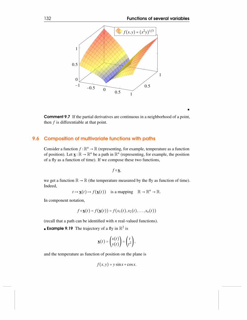
� Example 9.18 Consider the function
f (x,y) = (x2y)1�3For every direction v = (cosq ,sinq),
∂ f∂v(0,0) = lim
h→0
f (h cosq ,h sinq)− f (0,0)h
= cos2�3 q sin1�3 q ,
so that all the directional derivatives exist. In particular, setting q = 0,p�2,
∂ f∂x(0,0) = 0 and
∂ f∂y(0,0) = 0.
Is f differentiable at (0,0)? If it were, then by Proposition 9.2
∂ f∂v(0,0) = cosq ∂ f
∂x(0,0)+ sinq ∂ f
∂y(0,0),
which is not the case. Hence, we deduce that f is not differentiable at (0,0).
132 Functions of several variables
−1 −0.5 0 0.5 1
0.5
10
0.5
1
f (x,y) = (x2y)1�3
�Comment 9.7 If the partial derivatives are continuous in a neighborhood of a point,then f is differentiable at that point.
9.6 Composition of multivariate functions with paths
Consider a function f ∶Rn→R (representing, for example, temperature as a functionof position). Let x ∶R→Rn be a path in Rn (representing, for example, the positionof a fly as a function of time). If we compose these two functions,
f ○x,
we get a function R→R (the temperature measured by the fly as function of time).Indeed,
t � x(t)� f (x(t)) is a mapping R→Rn→R.
In component notation,
f ○x(t) = f (x(t)) = f (x1(t),x2(t), . . . ,xn(t))(recall that a path can be identified with n real-valued functions).
� Example 9.19 The trajectory of a fly in R2 is
x(t) = �x(t)y(t)� = � t
t2� ,and the temperature as function of position on the plane is
f (x,y) = y sinx+cosx.
9.6 Composition of multivariate functions with paths 133
Then the temperature measured by the fly as function of time is
f ○x(t) = f (x(t)) = t2 sint +cost.
�
The question is the following: suppose that we know the derivative of x at t (i.e.,we know the velocity of the path) and we know the derivative of f at x(t) (i.e., weknow how the temperature changes in response to small changes in position at thecurrent location). Can we deduce the derivative of f ○x at t (i.e., can we deduce therate of change of the temperature measured by the fly)?
Let’s try to guess the answer. For univariate functions the derivative of a compositionis the product of the derivatives (the chain rule), so we would guess,
d( f ○x)dt
(t) = f ′(x(t)) x(t).This expression is meaningless. The derivative of f is a vector and so is x′(t). Theleft-hand side is a scalar, hence an educated guess would be:
Proposition 9.3 — Chain rule. Let x ∶R→Rn and f ∶Rn→R be differentiableat t0 and at x(t0), respectively. Then f ○x is differentiable at t0 and
d( f ○x)dt
(t0) =∇ f (x(t0)) ⋅ x(t0).� Example 9.20 Let’s examine the above example, in which
∇ f (x) = �y cosx− sinxsinx
� and x(t) = � 12t� ,
so that
∇ f (x(t)) ⋅ x(t) = �t2 cost − sintsint
� ⋅� 12t� = t2 cost − sint +2t sint.
On the other hand,
d( f ○x)dt
(t) = t2 cost +2t sint − sint,
i.e., Proposition 9.3 seems correct. �
Proof. Since x is differentiable at t0 it follows that
x(t) = x(t0)+ x(t0)(t − t0)+o(�t − t0�),
134 Functions of several variables
which we may also write as
Dx = x(t0)Dt +o(�Dt �).Since f is differentiable at x(t0) it follows that
f (x(t)) = f (x(t0))+∇ f (x(t0)) ⋅Dx+o(�Dx�).Putting things together,
f (x(t)) = f (x(t0))+∇ f (x(t0)) ⋅ x(t0)Dt +o(�Dt �),which by definition, implies the desired result. �
9.7 Differentiability and implicit functions
Recall that a function x� f (x) may be defined implicitly via a relation of the form
G(x, f (x)) = 0,
where G ∶R2→R. Another way to state it is that f is defined via its graph
Graph( f ) = {(x,y) � G(x,y) = 0}.Suppose that (x0,y0) ∈ Graph( f ), i.e., y0 = f (x0). Consider now the directionalderivatives of G along v = (cosq ,sinq) at (x0,y0),
∂G∂ v(x0,y0) = v ⋅∇G(x0,y0) = cosq ∂G
∂x(x0,y0)+ sinq ∂G
∂y(x0,y0).
The line tangent to the graph of f at (x0,y0) is along the direction in which thedirectional derivative of G vanishes, i.e.,
∂G∂ v(x0,y0) = cosq �∂G
∂x(x0,y0)+ tanq ∂G
∂y(x0,y0)� = 0.
Thus,
f ′(x0) = tanq = − ∂G∂x (x0,y0)∂G∂y (x0,y0) .
� Example 9.21 Let G(x,y) = x2+y2−16 and (x0,y0) = (2,√12). Then,
∂G∂x(2,√12) = 4 and
∂G∂y(2,√12) = 2
√12,
so thatf ′(2) = − 4
2√
12= − 1√
3.
�
9.8 Interpretation of the gradient 135
9.8 Interpretation of the gradient
We saw that for every function f ∶Rn→R and unit vector v,
∂ f∂ v(a) = v ⋅∇ f (a).
∇ f (a) is a vector in Rn. What is its direction? What is its magnitude.
If q is the angle between the gradient of f at a and v, then
∂ f∂ v(a) = �∇ f (a)� cosq .
The directional derivative is maximal when q = 0, which means that the gradientpoints to the direction in which the function changes the fastest. The magnitude ofthe gradient is this maximal directional derivative.
Likewise,∂ f∂ v(a) = 0 when ∇ f (a) ⊥ v,
i.e., ∇ f (a) is perpendicular to the contour line of f at a.
� Example 9.22 Consider once again the distance function
f (x) = �x�.We saw that ∇ f (x) = x,
i.e., the gradient points along the radius vector (the direction in which the radiusvector changes the fastest) and its magnitude is one, as
∂ f∂ x= lim
h→0
f (x+hx)− f (x)h
= limh→0
�x+hx�− �x�h
= 1.
�
Definition 9.2 Let f ∶Rn→R. A point a ∈Rn at which
∇ f (a) = 0
is called a stationary point, or a critical point ( �;*)*98 %$&81).
What is the meaning of a point being stationary? That in any direction the pointwiserate of change of the function is zero. Like for univariate functions, stationary pointsof multivariate functions can be classified:
1. Local maxima: For every v ∈Rn, the function
g(t) = f (x0+ t v)has a local maximum at t = 0. Example, f (x,y) = −x2−y2.
136 Functions of several variables
2. Local minima: For every v ∈Rn, the function
g(t) = f (x0+ t v)has a local minimum at t = 0. Example, f (x,y) = x2+y2.
3. Saddle points (�4,&! ;&$&81): A stationary point that’s neither a local mini-mum nor a local maximum. Typically,
g(t) = f (x0+ t v)may have a local minimum, a local maximum or an inflection point at t = 0,depending on the direction v. Example, f (x,y) = x2−y2.
−1 −0.5 0 0.5 1 −1
0
1−1
0
1
f (x,y) = x2−y2
� Example 9.23 Consider the function
f (x,y) = x3+y3−3x−3y.
−1 01 −1
01−4
−2
0
2
4
f (x,y) = x3+y3−3x−3y
9.9 Higher derivatives and multivariate Taylor theorem 137
Its gradient is
∇ f (x,y) = �3x2−33y2−3� ,
hence its stationary points are (±1,±1).Take first the point a = (1,1). For v = (cosq ,sinq),
f (a+ t v) = (1+ t cosq)3+(1+ t sinq)3−3(1+ t cosq)−3(1+ t sinq).Expanding, we find
f (a+ t v) = −4+3t2 cos2 q +3t2 sin2 q +o(t2) = −4+3t2+o(t2),hence in every direction v, f (a+ t v) has a local minimum at t = 0. That is, a is alocal minimum of f .
Take next the point b = (1,−1). For v = (cosq ,sinq),f (b+ t v) = (1+ t cosq)3+(−1+ t sinq)3−3(1+ t cosq)−3(−1+ t sinq).
Expanding, we find,
f (b+ t v) = 3t2 cos2 q −3t2 sin2 q +o(t2),For q = 0, f (b+ t v) has a local minimum at t = 0, whereas for q = p�2, f (b+ t v)has a local maximum at t = 0. Thus, b is a saddle point of f .
�
9.9 Higher derivatives and multivariate Taylor theorem
Let f ∶R2→R. If f is differentiable in a certain domain, then it has partial deriva-tives,
∂ f∂x
and∂ f∂y
,
which both are also functions R2 →R (recall the the gradient is a function R2 →R2). If the partial derivatives are differentiable, then they have their own partialderivatives, which we denote by
∂∂x
∂ f∂x= ∂ 2 f
∂x2∂∂y
∂ f∂x= ∂ 2 f
∂x∂y∂∂y
∂ f∂y= ∂ 2 f
∂y2∂∂x
∂ f∂y= ∂ 2 f
∂y∂x.
More generally, for functions f ∶Rn→R, we have an n-by-n matrix of partial secondderivatives (called the Hessian),
∂ 2 f∂xi ∂x j
i, j = 1, . . . ,n.
138 Functions of several variables
Each such partial second derivative is a function Rn→R, which may be differentiatedalong any direction. A function Rn→R that can be differentiated infinitely manytimes along any combination of directions is called smooth ( �%8-().
Theorem 9.4 — Clairaut. If f ∶Rn→R has continuous second partial derivativesthen
∂ 2 f∂xi ∂x j
= ∂ 2 f∂x j ∂xi
.
That is, the matrix of second derivatives is symmetric.
Comment 9.8 This is not a trivial statement. One has to show that
limh→0
∂ f∂xi(x+h e j)− ∂ f
∂xi(x)
h= lim
h→0
∂ f∂x j(x+h ei)− ∂ f
∂x j(x)
h.
� Example 9.24 Consider the function,
f (x,y) = yx3+xy4−3x−3y.
Then,∂ f∂x= 3x2y+y4−3
∂ f∂y= x3+4y3x−3,
and
∂ 2 f∂x2 = 6xy
∂ 2 f∂y∂x
= 3x2+4y3 ∂ 2 f∂y2 = 12y2x
∂ 2 f∂x∂y
= 3x2+4y3.
We may calculate higher derivatives. For example,
∂ 3 f∂x∂y∂x
= 6x.
�
Suppose we know f ∶R2 →R and its derivatives at a point (x0,y0). What can wesay about its values in the vicinity of that point, i.e., at a point (x0+Dx,y0+Dy)? Itturns out that the concept of a Taylor polynomial can be generalized to multivariatefunction.
9.9 Higher derivatives and multivariate Taylor theorem 139
Definition 9.3 Let f ∶R2→R be n-times differentiable at x0 = (x0,y0). Then, itsTaylor polynomial of degree n about the point x0 is
Pf ,n,x0(x) = f (x0)+ ∂ f
∂x(x0)(x−x0)+ ∂ f
∂y(x0)(y−y0)
+ 12�∂ 2 f
∂x2 (x0)(x−x0)2+2∂ 2 f
∂x∂y(x0)(x−x0)(y−y0)+ ∂ 2 f
∂y2 (x0)(y−y0)2�+ ⋅ ⋅ ⋅+ n�
k=0�n
k� ∂ n f
∂xk ∂yn−x (x0)(x−x0)k(y−y0)n−k.
Theorem 9.5 Let f ∶R2→R be n-times differentiable at x0 = (x0,y0). Then,
lim�x−x0�→0
f (x)−Pf ,n,x0(x)
�x−x0�n = 0,
or using the equivalent notation,
f (x) = Pf ,n,x0(x)+o(�x−x0�n).
� Example 9.25 Calculate the Taylor polynomial of degree 3 of the function
f (x,y) = x3 lny+xy4
Then,∂ f∂x(x,y) = 3x2 lny+y4 ∂ f
∂y(x,y) = x3
y+4xy3,
∂ 2 f∂x2 (x,y) = 6x lny
∂ 2 f∂x∂y
(x,y) = 3x2
y+4y3 ∂ 2 f
∂y2 (x,y) = −x3
y2 +12xy2,
and
∂ 3 f∂x3 (x,y)=6lny
∂ 3 f∂x2 ∂y
(x,y)= 6xy
∂ 3 f∂x∂y2 (x,y)=−3x2
y2 +12y2 ∂ 3 f∂y3 (x,y)= 2x3
y3 +24xy.
At the point (1,1),Pf ,3,(1,1)(1+Dx,1+Dy) = 1+(Dx+5Dy)+ 1
2�14DxDy+11Dy2�
+ 16�18Dx2 Dy+27DxDy2+26Dy3� .
�
140 Functions of several variables
9.10 Classification of stationary points
Taylor’s theorem for functions of two variables can be used to classify stationarypoints. If a is a stationary point of f ∶R2→R and f is twice differentiable at thatpoint, then by Taylor’s theorem
f (a+Dx) = f (a)+ 12�∂ 2 f
∂x2 (a)Dx2+2∂ 2 f
∂x∂y(a)DxDy+ ∂ 2 f
∂y2 (a)Dy2�+o(�Dx�2).Near stationary points, f − f (a) is dominated by the quadratic terms (unless theyvanish, in which case we have to look at higher-order terms). To shorten notationslet’s write,
∂ 2 f∂x2 (a) = A
∂ 2 f∂x∂y
(a) = B and∂ 2 f∂y2 (a) =C,
i.e.,
f (a+Dx) = f (a)+ 12�ADx2+2BDxDy+CDy2���������������������������������������������������������������������������������������������������������������������������������������������������������
M(Dx)+o(�Dx�2).
Consider the quadratic term M(Dx):1. If it is positive for all Dx ≠ 0, then a is a local minimum.2. If it is negative for all Dx ≠ 0, then a is a local maximum.3. If it changes sign for different Dx, then a is a saddle point.
We now characterize under what conditions on A,B,C each case occurs:
1. M(Dx) > 0 for all Dx ≠ 0 if A,C > 0, i.e., if
∂ 2 f∂x2 (a), ∂ 2 f
∂y2 (a) > 0.
This is still not sufficient. Writing,
M(x) = �√ADx+ B√A
Dy�2+�C− B2
A�Dy2,
we obtain that AC > B2, i.e.,
∂ 2 f∂x2 (a)∂
2 f∂y2 (a) > � ∂ 2 f
∂x∂y(a)�2
.
9.11 Extremal values in a compact domain 141
2. M(Dx) < 0 for all Dx ≠ 0 if A,C < 0, i.e., if
∂ 2 f∂x2 (a), ∂ 2 f
∂y2 (a) < 0.
This is still not sufficient. Writing,
M(x)=−(�A�Dx2−2BDxDy+ �C�Dy2)=−����A�Dx− B��A�Dy
��
2
−�B2
�A� − �C��Dy2,
we obtain once again that AC > B2, i.e.,
∂ 2 f∂x2 (a)∂
2 f∂y2 (a) > � ∂ 2 f
∂x∂y(a)�2
.
3. A saddle point occurs if
∂ 2 f∂x2 (a)∂
2 f∂y2 (a) < � ∂ 2 f
∂x∂y(a)�2
.
We can see it by setting Dx = 1, in which case
M(1,Dy) = A+2BDy+CDy2,
which changes sign if the discriminant if positive.
To conclude:
Type Conditions
Local minimum ∂ 2 f∂x2 > 0 ∂ 2 f
∂y2 > 0 ∂ 2 f∂x2 ⋅ ∂ 2 f
∂y2 > � ∂ 2 f∂x∂y�2
Local maximum ∂ 2 f∂x2 < 0 ∂ 2 f
∂y2 < 0 ∂ 2 f∂x2 ⋅ ∂ 2 f
∂y2 > � ∂ 2 f∂x∂y�2
Saddle ∂ 2 f∂x2 ⋅ ∂ 2 f
∂y2 < � ∂ 2 f∂x∂y�2
� Example 9.26 Analyze the stationary points (±1�√3,0) of the function
f (x,y) = x3−x−y2.
�
9.11 Extremal values in a compact domain
142 Functions of several variables
Definition 9.4 A domain D ⊂Rn is called bounded if there exists a number Rsuch that ∀x ∈D �x� < R.
Comment 9.9 In other words, a domain is bounded if it can be enclosed in a ball.
Definition 9.5 A domain D ⊂Rn is called open if any point x ∈D has a neigh-borhood {y ∈Rn � �y−x� < d}contained in D. It is called closed if its complement is open, i.e., if any pointx �∈D has a neighborhood
{y ∈Rn � �y−x� < d}disjoint from in D. This means that if x ∈Rn is a point that has the property thatevery ball around x intersects D, then x ∈D.
In this section we discuss extremal points of continuous functions defined on abounded and closed domain D ⊂Rn. Such domains are called compact ( �*)85/&8).Why are closedness and boundedness important? Recall that every for univariatefunction, a function continuous may fail to have extrema if its domain is not closedor unbounded. Like for univariate functions we have the following results:
Theorem 9.6 Let f ∶D→R be continuous with D ⊂Rn compact. Then f assumesin D both minima and maxima, i.e., where exist a,b ∈D such that
∀x ∈D f (a) ≤ f (x) ≤ f (b).Furthermore, if f assumes a local extremum at an internal point of D and f isdifferentiable at that point then its gradient at that point vanishes.
� Example 9.27 Consider the function
f (x,y) = x4+y4−2x2+4xy−2y2
in the domain
D = {(x,y) � −2 ≤ x,y ≤ 2}.
9.11 Extremal values in a compact domain 143
−2 −1 0 1 2 −2
0
20
20
f (x,y) = x4+y4−2x2+4xy−2y2
We start by looking for stationary points inside the domain. The gradient is
∇ f (x,y) = �4x3−4x+4y4y3+4x−4y
� ,which vanishes for
y = x−x3 and x = y−y3,
i.e.,y = y−y3−(y−y3)3,
from gives y3 = y3(1−y2)3, i.e., y = 0 or y = ±√2, i.e., the stationary points are
a = (0,0) b = (−√2,√
2) and c = (√2,−√2).To determine the types of the stationary points we calculate the Hessian,
∂ 2 f∂x2 (x,y) = 12x2−4
∂ 2 f∂x∂y
(x,y) = 4 and∂ 2 f∂y2 (x,y) = 12y2−4.
I.e.,
H(a) = �0 44 0� H(b) =H(c) = �20 4
4 20� ,from which we deduce that a is a saddle point and b and c are local minima, with
f (b) = f (c) = −8.
We now turn to consider the boundaries, which comprise of four segments. Since fis symmetric,
f (x,y) = f (y,x) = f (−x,−y),
144 Functions of several variables
it suffices to check one segment, say, the segment {−2}× [−2,2], where f takes theform
y� 16+y4−8−8y−2y2.
This is a univariate function whose derivative is
y� 4y3−8−4y.
The derivative vanishes at y ≈ 1.5214. The second derivative is
y� 12y2−2.
Since it is positive at that point, the point is a local minimum. The function at thatpoint equals approximately 20.9.
Finally, we need to verify the values of f at the four corners:
f (2,2) = f (−2,−2) = 32 and f (2,−2) = f (−2,2) = 0.
To conclude f assumes its minimal value, (−8) at (−√2,√
2) and (√2,−√2), andits maximal value, 32, at (2,2) and (−2,−2). �
9.12 Extrema in the presence of constraints
9.12.1 Problem statement
The general problem: Let f ∶Rn→R and let also
g1,g2, . . . ,gm ∶Rn→R.
We are looking for a point x ∈Rn that minimizes or maximizes f under the constraintthat
g1(x) = g2(x) = ⋅ ⋅ ⋅ = gm(x) = 0.
That is, the set of interest is
{x ∈Rn � g1(x) = g2(x) = ⋅ ⋅ ⋅ = gm(x) = 0}.Without the constraints, we know that the extremal point must be a critical point ofx. In the presence of constraints, it may be that the extremal point is not stationarysince the directions in which it changes violate the constraints.
� Example 9.28 Find the extremal points of
f (x,y) = 2x2+4y2
under the constraintg(x,y) = x2+y2−1 = 0.
Note that f by itself does not have a maximum in Rn since it grows unbounded as�x�→∞. However, under the constraint that �x� = 1 it has a maximum. �
9.12 Extrema in the presence of constraints 145
9.12.2 A single constraint
Let’s start with a single constraint. We are looking for extremal points of f ∶Rn→Runder the constraint
g(x) = 0.
One approach could be the following: since the constraint is of the form
g(x1, . . . ,xn) = 0,
invert it to get a relation,xn = h(x1, . . . ,xn−1),
substitute it in f to get a new function
F(x1, . . . ,xn−1) = f (x1, . . . ,xn−1,h(x1, . . . ,xn−1)),which we then minimize without having to deal with constraints. The problem withthis approach is that it is often impractical to invert the constraint. Moreover, theconstraint may fail to define an implicit function (like in Example 9.28, where theconstraint is an ellipse).
The constrained optimization problem can also be approached as follows: the set
D = {x ∈Rn � g(x) = 0}over which we extremize f is in general an (n−1)-dimensional hyper-surface (acurve in Example 9.28). The gradient of g in D points to the direction in which gchanges the fastest. The plane perpendicular to this direction spans the directionsalong which g remains constant. f has an extremal point in D if the gradient of f isperpendicular to the hyperplane along which g remains constant. In other words, fhas an extremal point at x ∈D if the gradient of f is parallel to the gradient of g, i.e.,there exists a scalar l such that
∇ f (x) = l∇g(x).A equivalent explanation is the following: let x(t) be a general path in Rn satisfying
x(0) = x0.
The paths along which g does not change satisfy
g(x(t)) = 0.
For all such path, (g○x)′(0) =∇g(x(t)) ⋅x′(0) = 0.
x0 is a solution to our problem it for all such paths,
f (x(t)) has an extremum at t = 0,
146 Functions of several variables
i.e., ( f ○x)′(0) =∇ f (x0) ⋅x′(0) = 0.
This condition holds if ∇ f (x0) and ∇g(x0) are parallel.
Comment 9.10 Note that ∇ f (x0) and ∇g(x0) are parallel if and only if thereexists a number l such that x0 is a stationary point of the function
F(x) = f (x)−l g(x).In this context the number l is called a Lagrange multiplier ( �'19#- -5&,).
� Example 9.29 Let’s return to Example 9.28. Then, x = (x,y) is an extremal pointif there exists a constant l such that x is a critical point of
F(x,y) = �2x2+4y2�−l �x2+y2−1�Note,
∇F(x,y) = �4x−2lx8y−2ly
� ,i.e., either x = 0 (in which case y = ±1) and l = 4 or y = 0 (in which case x = ±1) andl = 2. To find which point is a minimum/maximum we have to substitute in f . �
9.12.3 Multiple constraints
For simplicity, let’s assume that there are just two constraints,
D = {x ∈Rn � g1(x) = g2(x) = 0}.let x(t) be a general path in Rn satisfying
x(0) = x0.
The paths along which g1 and g2 do not change satisfy
g1(x(t)) = g2(x(t)) = 0.
For all such path, (g1 ○x)′(0) =∇g1(x(t)) ⋅x′(0) = 0(g2 ○x)′(0) =∇g2(x(t)) ⋅x′(0) = 0.
x0 is a solution to our problem it for all such paths,
f (x(t)) has an extremum at t = 0,
i.e., ( f ○x)′(0) =∇ f (x0) ⋅x′(0) = 0.
9.12 Extrema in the presence of constraints 147
This condition holds if ∇ f (x0) is any linear combination of ∇g1(x0) and ∇g1(x0),i.e., there exists two constants, l and µ such that
∇ f (x0) = l∇g1(x0)+µ∇g2(x0),or equivalently, x0 is a stationary point of the function
F(x) = f (x)−l g1(x)−l g2(x).� Example 9.30 Find a minimum point of
��� .The condition that x be a stationary point of F imposes three conditions on fiveunknowns. The constrains provide the two missing conditions. We may first get ridof z = 1−x−y, i.e.,
2(1−µ)x = l 2(2−µ)y = l 2(3−µ)(1−x−y) = l
andx2+y2+(1−x−y)2 = 1.
We can then get rid of l ,
(1−µ)x= (2−µ)y (3−µ)(1−x−y)= (1−µ)x and x2+y2+(1−x−y)2 =1.