71
Instruction Manual for 90Plus/BI-MAS Multi Angle Particle Sizing Option Operation Manual Brookhaven Instruments Corporation 750 Blue Point Road Holtsville, NY 11742 Phone: (631) 758-3200
| Date post: | 03-Jan-2016 |
| Category: |
Documents |
| Upload: | jose-luis-guerra-jacome |
| View: | 51 times |
| Download: | 2 times |
Instruction Manual
for
90Plus/BI-MASMulti Angle Particle Sizing Option
Operation Manual
Brookhaven Instruments Corporation750 Blue Point RoadHoltsville, NY 11742
Phone: (631) 758-3200Fax: (631) 758-3255e-mail: [email protected]
www.bic.com

PLEASE READ
This is your instruction manual for the Brookhaven BI_MAS option. Please read it carefully before making measurements. The INSTALLATION section describes procedures for checking that the instrument and software are working properly. Familiarize yourself with the software by running the program with some of the data sets that are provided for this purpose. If you have any questions, comments or suggestions, please contact Brookhaven.
2

COPYRIGHT NOTICE
Copyright , 1994 by Brookhaven Instruments Corporation. All Rights Reserved Worldwide. No part of this Manual may be reproduced, transmitted, transcribed, stored in a retrieval system, or translated into any human or computer language, in any form or by any means, electronic, mechanical, magnetic, optical, chemical, manual or otherwise, without the express written permission of Brookhaven Instruments Corporation, Brookhaven Corporate Park, 750 Blue Point Road, Holtsville, NY 11742, U.S.A.
First Printing : January, 1995Catalog Number : MASMAN, Ver. 1.0
3

WARRANTYBrookhaven Instruments Corporation (hereinafter known as BIC) warrants that the product is free from defective material and workmanship. Under the terms of the warranty BIC agrees to correct by repair, or at BIC’s election by replacement, any parts which prove to be defective through no fault of the user.
This warranty is limited to the original purchaser of the product.
The product shall be shipped, freight prepaid and insured in full, or delivered to a facility authorized by BIC to render the service provided thereunder, in either the original package or in a similar package affording an equal degree of protection. The purchaser must contact BIC for instruction prior to returning the product.
The product shall not have been previously altered, repaired or serviced by anyone other than a service facility authorized by BIC. The product shall not have been subjected to accident, misuse or abuse, or operated contrary to the instructions contained in the instruction manual or manuals.
BIC shall not be liable for direct, indirect, incidental, consequential, or other type of damages resulting from use of this product other than the liability stated above. These warranties are in lieu of all other warranties, expressed or implied, including, but not limited to, the implied warranties of merchantibility or fitness for a particular purpose.
The BIC warranty extends for a period of 90 days. This period from the date of receipt of the equipment, and it applies only to the original purchaser. The warranty period is automatically extended to 1 year (except as noted below) from the date of receipt of the equipment provided all invoices for said equipment, including transportation, if applicable, are paid within 30 days after receipt of invoice.
The BIC warranty extends for a period not exceeding the warranty period of the Original Equipment Manufacturer where applicable. The typical warranty period on printers and computer peripherals is 90 days. Please contact BIC for copies of applicable OEM warranties.
4

Software License Agreement
Carefully read the following terms before using the software provided with the system. Use of the software indicates your acceptance of these terms. If you do not agree with the terms, promptly return the software and the system. BIC refers to Brookhaven Instruments Corporation.
Terms
1. In purchasing this software you are granted non-exclusive license to use the software product on one computer.
2. BIC retains title to, and ownership of, the software product. The software product may not be modified without the express written consent of BIC.
3. Duplication of the software product for any purpose other than backup protection, including for any commercial use, is a violation of the copyright laws of the United
States of America and of other countries. Information produced by using BIC software and its manual, including the resulting displays, reports and plots are believed to be accurate and reliable. However no responsibility is assumed by BIC for any changes, errors, or omissions.
5

Table of Contents
I IntroductionI.1 References
II Installation
III The MAS option SoftwareIII.1 Loading DataIII.2 ParametersIII.3 Copy to ClipboardIII.4 GraphsIII.5 Collecting New DataIII.6 Multiple MeasurementsIII.7 Data FilesIII.8 Printer Support
IV QELS TheoryIV.1 Light ScatteringIV.2 What Causes Light ScatteringIV.3 CorrelationIV.4 Basic EquationsIV.5 References
V Data InterpretationV.1 PreliminariesV.2 Narrow Distribution of SpheresV.3 Broad Distribution of Spheres
V.3.1 Fit to a known DistributionV.3.2 Cumulant Analysis
V.4 Nonspherical ParticlesV.5 Advanced Data InterpretationV.6 References
6

Appendix ICompatibility of common liquids with acrylic cells
Appendix IIRaw Data File Format
Appendix IIIText File Report
Appendix IVOperating Environment Definitions
BI9K.INI9KPSDW.INI
Appendix VIndex of Refraction of Particles
7

I Introduction
The MAS OPTION is an automatic particle sizer designed for use with either concentrated suspensions of small particles or solutions of macromolecules. Generally speaking, sizes from 2nm to 3m can be measured. The software for instrument control and data analysis is written for use in the Microsoft Windows environment though a DOS version is also available.
The technique employed - photon correlation spectroscopy (PCS) of quasi-elastically scattered light (QELS) - is based on correlating the fluctuations about the average, scattered, laser light intensity. It has several advantages including:
Speed (Typically 1 to 2 minutes) Accuracy ( 1% on monodisperse samples) Sample Volume (0.5 to 3 ml) Calibration (None required) Versatility (Measures particles, polymers, emulsions, colloids,
etc. in any suitable liquid)
Sample preparation is relatively quick and easy with dust being the major problem. Using a few simple “tricks of the trade” and the unique built in “dust filter” will allow a high percentage of acceptable measurements to be made by the novice user.
Computer control of the MAS OPTION makes the instrument easy to operate. The software is menu driven with friendly screens designed to guide and inform at each stage of the operation. Common problems are identified and accentuated and simple remedies are suggested by the software. After pressing the Start button, everything else is automatic, including the calculations.
Please read the chapters on Installation, Self Test, the MAS OPTION
Software and Diagnostics before attempting to use the instrument. The chapters entitled Quasi Elastic Light Scattering (QELS) Theory and Data Interpretation are not essential for correct instrument setup and operation. However, an understanding of these principles will help the user to apply the results in a better informed fashion.
The technical and sales personnel at Brookhaven would be glad to render any assistance regarding questions that you might have about the MAS OPTION that have not been clarified despite reading this manual.
8

I.I Specifications
Size Range : 2nm to 3m
Diffusion Coefficient Range : 10-6 to 10 -9 cm2/sec
Accuracy : 1% to 2% with monodisperse samples
Repeatability : 1% to 2% with dust free samples
Laser : 15mW solid state laser. Complies with BRH 21CFR 1040:10 as applicable.
TemperatureControl (OPTIONAL) : 5 C to 75 C on steps of 0.1 C
Sample Volume : 0.5 to 3ml
Measurement Time : Typically 1 to 2 minutes
Results : Mean and Standard Deviation calculated for size distribution by weight assuming a
Lognormal distribution. All results are displayed on the monitor and can be printed. Text file reports are provided and the raw data can be exported into an ASCII text file as well. Multimodal Size Distribution analysis (MSD) is optional.
9

II Installation
To install the MAS OPTION particle sizing software in Windows:
1) Insert the install diskette into the drive (for example in a:).2) From the Windows File menu select Run...3) The Run dialog box will appear as shown in Figure (2a)
Figure 2aThe Run dialog box in Windows
4) Run setup.exe by entering it on the command line preceded by the drive letter.
a:>\setup
The software will be installed in the sub-directory 9KPSDW in the directory BICW. It is strongly recommended that the installation directories be allowed to remain as named by the setup software and not be altered in any way.
A data directory for the storage of measurement data will also be created. This will be a sub-directory of the 9KPSDW directory called DATA.
To install the Multimodal Size Distribution (MSD) software (or to update the version of the MAS OPTION software at a later time) insert the MSD (or the updated MAS OPTION software diskette) diskette into the drive and follow steps 1 through 4 as before.
Note: To execute the Windows particle sizing program from DOS please type SIZE at the DOS prompt.
II.3 Self test
As we have discussed at various points in this manual, the heart of the MAS OPTION is a digital autocorrelator that processes information for the instrument and
10

generates an autocorrelation function. It is from this function that vital information such as particle size and polydispersity are obtained. The correlator is equipped with self diagnostic capabilities. Before attempting to make a measurement, it is advisable to use these self-test functions to ascertain that the correlator is functioning properly. To execute the diagnostics, press Ctrl+T in the main menu of the program. This puts the correlator into its test mode wherein it correlates 200 channels linearly spaced from 5 micro seconds to 1 second and accumulates for 5 seconds. At the end of this test procedure, the screen should look like the one shown in figure (2b).
Figure 2bTesting the correlator
11

III The MAS OPTION Software
The software for your Brookhaven MAS OPTION has been designed to run in the Microsoft Windows environment. Users who wish to familiarize themselves with Microsoft Windows should read their Windows documentation before attempting to use the MAS OPTION software.
The MAIN MENU for the MAS OPTION software is the menu page through which all the features of the software can be accessed. Figure (3a) shows the MAIN MENU as it appears when the program is first executed.
Figure 3aThe Main Menu
Before we begin taking any new data, let us familiarize ourselves with the operation of the software by learning how to load a data set and how to analyze it. As mentioned before, the software is designed to be compatible with the philosophy behind most Windows based programs. The menu bar is located at the top of the MAIN
12

MENU and remains accessible so long as the window bearing the MAIN MENU is active. To access a data file one needs to go through the following simple steps:
III.1 LOADING DATA
Move the mouse cursor over to File on the Menu bar of the MAIN MENU and click on it. The File menu will now become accessible:
Figure 3bThe File Menu
Selecting the Utilities option in this menu will open the File Utilities page (Figure 3c) and afford access to the data files stored in the various folders. The buttons on the bottom of the page give you access to the various features of this menu.
1. Select a Folder by clicking on it.
A list of files stored in that folder appear.
2. Select a file by clicking on it.
The buttons on the screen are now active pertaining to the file and/or the folder that you have selected. Files can be opened (Open File - you can also do this by double-clicking on any file) or deleted (Delete File - this becomes active when a file has been selected You will be asked for confirmation before the file is actually deleted). You can also create a folder (Create Folder - you will be prompted for a folder name limited to 30 characters), delete a folder (Delete Folder - this becomes active when a folder has been selected, again you will be asked for confirmation), import a folder ( Import Folder) from another directory or from a disk and export a folder (Export Folder) to another directory or to a floppy disk.
13

In this case, we see that two folders exist. Folder 1 has nothing in it, it is meant to store any new data that you may generate. At the present time, the folder called Sample Data is of more interest to us. We can select this folder by double clicking on it. We can now see a list of the data files that are stored in the folder Sample Data (Figure 3c). The data is identified primarily by the Sample Id though the automatically attached Date and Time stamp can also be used for this purpose. A Batch number may also be provided by the user for additional identification. Let us select the first sample.
Double click on Duke 96nm Standard.
We have now loaded the data associated with the Duke 96nm Standard sample.
Figure 3cThe File Utilities Page
Figure 3d shows the screen that results from loading a data file. The results appear conveniently tabulated just below the Sample Id. Each of these quantities are discussed in greater detail in the chapter on Data Interpretation. For now we will accept them at face value keeping in mind that the Effective Diameter represents an average size of the particles in the sample and that the Polydispersity is a measure of the non-uniformity’s that exist in the particle size distribution, Avg. Count Rate is a measure of signal intensity (Kilo Counts Per Second - KCPS) and Sample Quality is an indicator
14

of the difference between the measured and calculated baselines of the correlation function. The highest number (best quality) is 10.
Figure 3dA reloaded data set is displayed on this screen.
At the bottom of the screen are six buttons, each affording access to additional features of the software.
The Start, Clear and Runs buttons pertain to collecting data from your sample. For the time being we will leave it at that and return to them later.III.2 Parameters
The Parameters button provides us access to the Parameter page as shown in Figure 3e. This page serves the twofold purpose of sample archiving as well as entering the parameters needed for running the sample and for data analysis. Let us examine these a little more closely:
Sample ID : Enter the name by which you wish to identify your sample. (30 characters maximum).
15

Operator ID : Enter your name (30 characters maximum).
Notes : Enter any notes that you might have on this sample (42 characters maximum).
Batch # : Enter a Batch Number for your samples (5 Digits maximum)
Runs : Enter the number of successive runs you wish to make on this sample.
Run Duration: Enter the desired duration for each run.
The preceding parameters are mainly archival in nature and are optional. The following however, are used for calculations and should be entered with due care.
Temp.: Enter the temperature at which the sample will be controlled.Suspension : Enter the medium in which the sample is suspended. A list of common
media is made available by clicking on the symbol.
Viscosity : The viscosity of the medium (Automatically calculated from the temperature).
Ref. Index : The Refractive Index of the medium (Automatically calculated and inserted).
Refractive Index of Particles
Real : Real component of the particle refractive index.
Imaginary : Imaginary component of the refractive index.
Enabling the Auto Save Results feature (by clicking in the box) will result in the results being saved at the end of every run. If the Auto Save Results feature is not turned on, you will have to manually save the data after each run.
16

Figure 3eThe Parameters Page
To save any changes that you make to the Parameters Menu, click on the OK button, to exit without saving any of the changes, click on the Cancel button.
III.3 Copy to Clipboard
This is a very useful feature for transporting results from one Windows
application to another. By clicking on this button the data represented on the screen (both tabular and graphical) is copied to the Windows clipboard. It can now be exported to any application by using standard Windows clip and paste techniques. For example you could incorporate a graph or a table into a document created by using Microsoft Word for Windows.
17

III.4 Graphs
This button allows you to change the screen to either add a graphical representation of the data, or to erase the graph if one is already present. Once the Graphs feature has been activated, you can select the type of graph to view.
The simplest graphical representation available is the Log Normal where the Effective Diameter and the Polydispersity are used to generate a log normal distribution of particle sizes.
You can click on MSD to see a more sophisticated representation of the size distribution. The MSD uses the Non-Negatively constrained Least Squares (NNLS) algorithm to fit the data. This is a model independent technique and it is possible to achieve multi-modal distributions using it.
Clicking on the Corr. Funct. will display the autocorrelation function obtained from the sample. This is the primary result measured by the instrument and all the other information is computed from this curve. A more detailed description of the correlationfunction is given in the chapter dealing with the theory of the MAS OPTION.
Clicking on the Zoom button will allow you to examine whichever graph that you might be viewing in greater detail (Figure 3f). In this expanded screen, it is possible to move the cursor along the curve to examine, at each point, the values of the x and y axes. A feature that some users might find useful is the ability to hide (or display) the cursors and the numerical values of the axes. Clicking on any portion of the Graphs
window outside the rectangle bounding the graph itself will hide the cursors and the data associated with the graph. Clicking inside the graph itself will restore the graph highlight and the data values. Again the Copy to Clipboard button will enable you to transport the graph to other Windows applications.
18

Figure 3fZooming into a graph
Clicking on the MSD Summary button will show a table of particle sizes and the corresponding values of intensity weighted sizes obtained from the NNLS algorithm (Figure 3g).
19

Figure 3gMSD table
III.5 Collecting New Data
Before beginning to seriously collect data with the instrument, it is usually a good idea to make a few trial measurements on a well known sample. A latex particle size reference material is well suited for this purpose and we recommend the 96nm latex manufactured by Duke Scientific Corporation.
We are now ready to attempt a trial measurement.
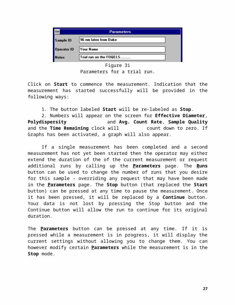
Clear any Data that might already be loaded into the MAS OPTION software. You can do this by clicking on the Clear button in the Main Menu screen. Click on Parameters page and enter the Parameters as discussed earlier. To start with it might be a good idea to leave most of the Parameters in their default settings and entering only the Sample ID, User ID and Notes.
Figure 3iParameters for a trial run.
Click on Start to commence the measurement. Indication that the measurement has started successfully will be provided in the following ways:
1. The button labeled Start will be re-labeled as Stop.2. Numbers will appear on the screen for Effective Diameter, Polydispersity and Avg. Count Rate, Sample Quality and the Time Remaining clock
will count down to zero. If Graphs has been activated, a graph will also appear.
If a single measurement has been completed and a second measurement has not yet been started then the operator may either extend the duration of the of the current measurement or request additional runs by calling up the Parameters page. The Runs button can be used to change the number of runs that you desire for this sample - overriding any request that may have been made in the Parameters page. The Stop button (that replaced the Start button) can be pressed at any time to pause the measurement. Once it has been pressed, it will be replaced by a Continue button. Your data is not lost by pressing the Stop button and the Continue button will allow the run to continue for its original duration.
20

The Parameters button can be pressed at any time. If it is pressed while a measurement is in progress, it will display the current settings without allowing you to change them. You can however modify certain Parameters while the measurement is in the Stop mode.
Allow the measurement to run for its complete duration. You should now be able to examine the results and satisfy yourself that they are acceptable.
III.6 Multiple Measurements
Figure 3j shows the screen when multiple measurements of a sample have been requested. You will notice that the lower part of the screen has been re-structured to incorporate a data table. This displays a brief “history” of the runs completed thus far along with some simple statistics showing the Mean and the Standard Error of the results.
Individual measurements may be deactivated from this table. You can deactivate a particular measurement either by double clicking on it or by pressing the number associated with the run. This will cause it to be grayed out in the table and its values will not contribute to the computation of the statistics for the table. Double clicking (or pressing the number) on a deactivated measurement will reactivate it.
21

Figure 3jMultiple Measurements. Run 2 has been deactivated.
Another feature that becomes available during multiple measurements is the Show Combined button. If the Show Combined button is clicked the program combines all the measurements into a single data set. It is as if the data from all the runs had been accumulated during the process of a single measurement. Obviously the Show Combined feature is possible only when more than one measurement is available. Once the Show Combined button is selected, it will be replaced by the Show Current button which enables the user to return to viewing the data from the most recent measurement.
The combined data should not be confused with the Mean displayed in the statistics. The Mean is an average of the completed measurements that are still activated. The combined data is generated by using the sum of the raw data from all of the completed measurements (that are activated) and recalculating the cumulant values. Also, to avoid confusion, note that while a measurement is in progress, the information in the upper portion of the screen is updated with data from both the current and the completed measurements that are activated. The information shown in the table in the lower portion of the screen is made up of completed measurements only.
22

III.7 Data Files
The MAS OPTION particle sizing software has a complete file system which maintains as many as 250 "folders" that may be used to store up to 500 data files each. A data file may contain as many as ten measurements of a single sample. Data files are saved automatically if the "autosave" option is selected in the parameters dialog. Files are always saved in the current active folder. When the program is installed the active folder is called Folder 1.
Data files are stored in a binary format and cannot be modified by the user. When a data file is saved, a copy of the Sample ID, date and time of the first measurement are saved in a folder file index. If a file is saved again after additional measurements of the same sample are made (without clearing previously measured data), then the same file will be updated to contain all the completed measurements.
The user may choose Save As from the file menu to save an additional copy of the current data. If the file is re-saved under a new name, then the new name is assumed to be a new sample identification. If previously saved, the original file will still exist under the previous sample identification. The operator may choose to save the file
Figure 3k
Saving Files
in a different folder or may even create a new folder from the Save As dialog. The folder chosen will become the current active folder and any further saved data will be placed in the current active folder.
You can also save the data in text format from the Save As dialog by selecting the Export button. The software will prompt the operator for the name and location of the text file to be generated. If more than one measurement has been completed, then
23

all active measurements will be combined into a single measurement including all the data from all the completed measurements. If multiple measurements have been completed, and an operator wants to save data from a single measurement then all other measurements should be deactivated before Exporting the data file. A deactivated measurement will appear gray on the main screen. Active measurements appear in red. The format of the data file generated is described in appendix I.
Figure 3l
Saving Files in various formats
Figure 3m
Saving data as a Text File Report
Clicking on the Text File Report button will provide you with a report of the results for the sample in standard ASCII text format. You will be prompted for a file name (for the text report). A example of a Text File Report is shown in appendix II.
24

An operator may save the current data at any time by choosing "Save" from the file menu. If no measurements have been completed then a partial measurement will be saved reflecting the current elapsed time. If one or more measurements have been completed then only completed measurements will be saved. Any partial measurements started after the first run is completed must also be completed in order to be included in the data file.
Data file folders may be maintained by choosing Utilities from the File menu on the main screen (Figure 3c). A dialog box will appear showing a list of folders and files. The current active folder is indicated by the open folder icon displayed to the left of the folder name. Please note that data folders do not correspond to individual DOS directories and all folders are maintained through software indexing exclusively. The files list box show files that have been stored under the current active folder only. Files stored in other folders will only be listed if the alternative folder is selected by "double clicking" the desired folder name in the folders list box.
Pressing the tab and shift-tab keys will move the focus of the dialog box from item to item. When the focus is placed in the folders list box, the currently selected item will be highlighted. This should not be confused with the current active folder which is marked with the "open folder" icon.
If the folder list box is selected, pressing the Delete Folder button will allow the user to delete the entire highlighted folder and all of the data file contained in it. Similarly, if the files list box show one or more selected files they may be deleted by pressing the "Delete File" command button. The operator will be given one chance only to verify the intention to delete files or folders. After that there is no way to recover deleted information.
Multiple files may be selected by pressing the Ctrl key while "single clicking" an individual file. A contiguous section of the file list may be selected by single clicking the first file and then the last file desired while pressing the shift key.
Files may be moved from one folder to a new folder by "dragging" the currently selected files to the new folder and "dropping" then into the new folder.
Files may be copied to a new folder by "dragging" the currently selected files to a new folder, while pressing the Ctrl key, and "dropping" them into the new folder.
25

Users should be aware of the current active folder because any further data
saved will be placed in this folder until the active folder is changed.
Occasionally, one or more data file will become damaged and will not be able to be reloaded by the software. This could happen for a variety for reasons including unexpected power interruption during a save operation. If this occurs, then the file list may inaccurately represent the available data file by displaying the names of un-readable sample data files. If the operator suspects that any data corruption has occurred, then the Rebuild Data File Index option should be invoked from the File menu. This will initiate a routine where the software will attempt to validate all data files and rebuild the appropriate folder index which will include only valid readable data files.
The File Utilities dialog also supports the archiving of complete file folders through use of the "Export Folder" command button. When selected, the user will be asked where to save a copy of the data included in the current highlighted folder.
The output of the export folder option is a binary file that contains all the sample data from all measurements included in the folder. The file is generated with a file extension of ".FDR". The file is saved in a binary format that is not compatible with any other software or word processors. Do not confuse this binary format with the text format used by the Export option available in the Save As dialog.
An operator may import the exported data folder back into the current highlighted folder by choosing the Import Folder button.
The import/export features can be used as a safety measure in order to "back up" your data files. It is also a convenient method of transporting data files from one computer to another.
III.8 Printer Support
All printer output must use standard window printer drivers and it is assumed that a printer has been previously installed through the Windows control panel. The standard Windows print setup and print preview dialogs are supported. Printer output can only be generated correctly on a printer that supports bitmap graphics and True Type fonts.
The software has the ability to generate a variety of printed data. The operator may select the type of data to output by choosing Printer Options from the File menu, and selecting the items of interest .
26
The most common printer output format used is the "Results Summary" which includes the information displayed on the main screen as well as the parameters in effect when the measurement was made. When printing the results summary, the current graph displayed on the main screen will be included in the results summary page. If no graph is displayed on the main screen then no graph will be included on the results summary page.
If more than one additional graphs are to be printed, they may be printed on a single page or on separate pages.
Please note that the date/time printed on each page header is the date/time of when the measurement was made and not the data/time of when the data is being printed.
27

IV Quasi Elastic Light Scattering (QELS) - Theory of Operation
IV.1 Light Scattering
The information in this chapter is not necessary for operating the MAS OPTION
particle sizer. If the operating instructions are followed correctly, good results will be obtained. However, if you wish to understand the basis for the measurement, and if you wish to interpret the results in a better informed fashion, then this chapter may be of considerable value.
Of the many techniques available for particle sizing light scattering offers many advantages: speed, versatility, small sample size, non-destructive, and measurement time independent of particle density. For sub-micron sizes it is sometimes the only viable technique.
IV.2 What Causes Light Scattering?
A little over a hundred years ago J.W. Strutt answered that question, and, in doing so, also answered the age-old question of why the sky is blue. Strutt became Lord Rayleigh, and the basics of light scattering were laid.
Light may be treated as an electro-magnetic wave. The oscillating electro-magnetic field induces oscillations of the electrons in a particle. These oscillating changes form the source of the scattered light.
Over the years many features of the scattered light have been used to determine particle size. These include:
Changes in the average intensity as a function of angle. Changes in the polarization. Changes in the wavelength. Fluctuations about the average intensity.
This later phenomenon is the basis for QELS, the technique employed in the MAS OPTION, and it arises in the following manner: imagine a detector of light fixed at some angle with respect to the direction of the incident light beam and at some fixed distance from the scattering volume which contains a large number of particles. Scattered light from each particle reaches the detector. Since the small particles are moving around randomly in the liquid, undergoing diffusive Brownian motion, the distance that the scattered waves travel to the detector varies as a function of time. Electromagnetic waves, like water and sound waves, exhibit interference effects. Scattered waves can interfere constructively or destructively depending on the distances traveled to the detector. The result is an average intensity with superimposed fluctuations. Figure 5a illustrates this.
28

Figure 5aFluctuations about the average scattered intensity.
The decay times of the fluctuations are related to the diffusion constants and, therefore, the sizes of the particles. Small particles moving rapidly cause faster decaying fluctuations than large particles moving slowly. The decay times of these fluctuations may be determined either in the frequency domain (using a spectrum analyzer) or in the time domain (using a correlator). The correlator generally offers the most efficient means for this type of measurement.
IV.3 Correlation
The concept of correlation is familiar to most people. If two variables or two signals are highly correlated then a change in one can be used to predict, with confidence, the change in the other. Mathematically, correlation is defined as the average of the products of the two quantities. Autocorrelation is just the average of the product of variable with a delayed version of itself.
In QELS the total time over which a measurement is made is divided into small time intervals called delay times. These intervals are selected to be small compared with the time it takes for a typical fluctuation to relax back to the average. The scattered light intensity in each of these intervals, as represented by the number of electrical pulses registered during each delay time, fluctuates about a mean value. The intensity autocorrelation function is formed by averaging the products of the intensities in these small time intervals as a function of the time between the intervals (delay times).
A computer automatically controls the buildup of the function including the choice of delay times, the length of the experiment, display of pertinent information, data
analysis, and the printing of results.
The Brookhaven MAS OPTION has several advantages over conventional QELS
systems:
29

The delay time intervals are not linearly spaced (in the default mode). This allows broad distributions to be sampled properly.
An algorithm is provided which removes signals affected by dust.
Unimodal fits to an assumed lognormal size distribution is standard. This distribution is the single most common one used in particle sizing. Multimodal and model independent size distribution software is
also available as an option.
Automatic repetition of measurements with statistical averaging is provided.
The software is Windows based with easy to use graphical user interfaces.
IV.4 Basic Equations
As described earlier, the random motion of small particles in a liquid gives rise to fluctuations in the time intensity of the scattered light. The fluctuating signal is processed by forming the autocorrelation function, C(t), t being the time delay. As t increases correlation is lost, and the function approaches the constant background term B. For short times the correlation is high. In between these two limits the function decays exponentially for a monodisperse suspension of rigid, globular particles and is given by
C(t) = A e-2 t + B 5-1
where A is an optical constant determined by the instrument design, and is related to the relaxation of the fluctuations by,
= D q2 [rad/sec] 5-2
The value of q is calculated from the scattering angle (eg. 90), the wavelength of the laser light o (eg. 0.635 m), and the index of refraction n (eg. 1.33) of the suspending liquid. The equation relating these quantities is
qn
Sin2
220
( ) 5-3
The translational diffusion coefficient, D, is the principle quantity measured by QELS. It is an inherently interesting property of particles and macromolecules. QELS has become the preferred technique for measuring diffusion coefficients of sub-micron particles.
30

Notice that no assumption about particle shape has to be made in order to obtain D other than assuming a general globular shape. Not until needle shape
particles have aspect ratios of greater than about 5, will a rotational diffusion term appear in the equation (1).
Particle size is related to D for simple common shapes like a sphere, ellipsoid, cylinder and random coil. Of these, the spherical assumption is most useful in the greatest number of cases. For a sphere,
Dk T
t dB
3 ( )[cm2/sec] 5-4
Where kB is Boltzmann’s constant (1.3805410-16 ergs/deg), T is the temperature in K, (t) (in centi poise) is the viscosity of the liquid in which the particle is moving, and d is the particle diameter. This equation assumes that the particles are moving independently of one another.
In summary, the determination of particle size consists of:
Measurement of the autocorrelation function. Fitting the measured function to equation (5-1) to determine . Calculating D from equation (5-2) given n, , and . Calculating particle diameter d from equation (5-4) given T and .
The MAS OPTION makes the measurements, fits the function, calculates D and d automatically. The measured autocorrelation function is more complex than equation (1). A preliminary discussion of the techniques used for handling polydisperse systems
is included in the chapter on Data Interpretation.
IV.5 ReferencesFor more information on laser light scattering consult the following references:
1) B. Chu, “Laser light scattering”, Academic Press, New York, 1974
2) B. Berne and R. Pecora, “Dynamic light scattering with applications to chemistry, biology and physics”, Wiley-Interscience, New York 1976
3) B.B. Weiner, W.W. Tscharnuter “Uses and Abuses of PCS in Particle Sizing”, in Particle Size Distribution, Assessment and Characterization, edited by Theodore Provder, ACS symposium Series 332, 1987.
4) H. Dhadwal, R. Ansari and W. Meyer, Rev. Sci. Instrum., 62 (12), 2963, (1991).
5) H. Dhadwal et al, Proc. S.P.I.E., 16,1884, 1993
31

V DATA INTERPRETATION
V.1 Preliminaries
The type of diameter obtained with photon correlation spectroscopy (PCS) is the hydrodynamic diameter (the particle diameter plus the double layer thickness) which is the diameter that a sphere would have in order to diffuse at the same rate as the particle being measured. This diameter may also be called the equivalent sphere diameter (ESD).
When a distribution of sizes is present, the effective diameter measured is an average diameter which is weighted by the intensity of light scattered by each particle. This intensity weighting, which is discussed below, is not the same as the population or number weighting used in a single particle counter such as in electron microscopy. However, even for narrowly dispersed samples, the average diameters obtained are usually in good agreement with those obtained by single particle techniques.
V.2 Narrow Distribution of Spheres
For monodisperse, rigid spheres the measured autocorrelation function (ACF) determined using the MAS OPTION is analyzed using eqs. 5-1, 5-2, 5-3, and 5-4.
How accurate are these equations and the MAS OPTION? Standard Reference Material (SRM) 1691 was obtained from the U.S. National Institute of Standards and Technology (NIST). The number average diameter, as determined by transmission electron microscopy (TEM) calibrated using NBS SRM 1690, is stated as 269 +/- 7nm, where the uncertainty includes both systematic and random errors as well as sample-to-sample variations. The MAS OPTION results are 273 +/- 5nm, where the uncertainty represents the average of 5 repeated measurements with 2 more measurements rejected as obvious outliers.
These measurements show that the MAS OPTION is capable of very accurate measurements on monodisperse spheres. (Please note that so-called standard latexspheres from other sources are not usually as well-known as the NBS SRM's, regardless of what is printed on the bottle.) It is also obvious from the uncertainty of the NBS standard that attempts at or claims of accuracy better than +/- 2.6% (7/269) are suspect.
32

V.3 Broad Distribution of Spheres
When a broad distribution of spheres is present in the sample eq. 5-1 must be modified before data analysis of the measured ACF can proceed. Each size contributes its own exponential, and the mathematical problem becomes
g t G e dt( ) ( ) 6-1
Here the baseline B of eq. 5-1 has already been subtracted and the square root of the remaining part has been taken eliminating the factor of 2 in the exponent.
The left hand side of eq. 6-1 is the measured data, and the desired distribution information, G( ), is contained under the integral sign on the right hand side. The solution to this Laplace Transform equation is nontrivial. The ill-conditioning of this transform, combined with measurement noise, baseline drifts and dust make the function particularly difficult to solve. It is therefore imperative to acquire the best possible statistics for the purposes of the measurement.
Several schemes have been proposed for obtaining information from eq. 6-1. These schemes may be grouped as follows:
Fit to a known distribution.
Cumulant analysis.
Inverse Laplace Transform.
V.3.1 Fit to a known distribution.
This method requires the assumption of a particular distribution. For example, if it is assumed that the distribution consists of only 2 peaks, each of which is very narrow, then eq. 6-1 reduces to the sum of 2 exponentials. The measured ACF is then fit to this sum of exponentials. The ratio of the fitted, pre-exponential factors contains information on the ratio of scattered intensities for each of the 2 peaks. And, in turn, this ratio of intensities can be related to the mass ratio for the two peaks. Likewise, the fitted 's contain information on the diameters of the 2 peaks.
33

The principal problem with this approach is the assumption of a given form (here, bimodal) for the distribution. One might think that different models (unimodal, bimodal, trimodal, etc.) could be compared using a statistical criteria such as a goodness-of-fit parameter like chi-squared. Unfortunately it is well-known that this approach often leads to ambiguous results with ill-conditioned equations like eq. 6-1.
An alternative approach is to assume an analytic equation for the distribution, integrate eq. 6-1 (numerical integration is usually required), and fit the results to the measurements. Typical analytic equations may have 2 or 3 parameters which are to be determined by the fitting. This approach again suffers from the assumption of a particular form of the distribution and has generally not proven successful.
V.3.2 Cumulant analysis.
The method of cumulants is more general (1). An understanding of this method provides the user with an insight into the "intensity" weighted character of the results from PCS. Cumulant results are very often reported in the scientific literature. They are often the starting point for further analysis. During a measurement with the MAS OPTION the cumulant results (effective diameter and polydispersity index) are calculated and displayed on an ongoing basis. Finally, the 2 cumulants are used to calculate the 2 lognormal parameters.
In the method of cumulants no assumption is made about the form of the distribution function. The exponential in eq. 6-1 is expanded in a Taylor series about the mean value. The resulting series is integrated to give a very general result. This result shows that the logarithm of the ACF can be expressed as a polynomial in the delay time, t. The coefficients of the powers of t are called the cumulants of the distribution. In practice, only the first couple of cumulants are obtained reliably, and these are identical to the moments of the distribution. (In general, the first moment of any distribution is the average and the second is the variance.)
The first two moments of the distribution G( ) are as follows:
= Dq2 6-2
2=(D2*-D*2)q4 6-3
where q is the scattering vector given in eq. 5-3 and D* is the average diffusion coefficient.
34

The effective diameter (hereinafter designated dpcs) is calculated from D using
equation 5-5.
Equation 6-3 shows that 2 is proportional to the variance of the "intensity"
weighted diffusion coefficient distribution. As such it carries information on the width of the size distribution. The magnitude and units of 2 are not immediately useful for
characterizing a size distribution. Furthermore, distributions with the same relative width (same shape) may have very different means and variances. For these reasons a relative width (reduced second moment) is conveniently defined as follows:
Polydispersity = 2/ 2 6-4
Polydispersity (Poly) has no units. It is close to zero (0.000 to 0.020) for monodisperse or nearly monodisperse samples, small (0.020 to 0.080) for narrow distributions, and larger for broader distributions.
Now lets examine the "intensity" weighting of the averaging process.
The intensity of light scattered by a suspension of particles with diameter d is proportional to the number of particles N, the square of the particle mass M, and the particle form factor P(q,d) which depends on size, scattering angle, index of refraction, and wavelength. Using "intensity" weighting, the following equations may be derived for the moments of the diffusion coefficient distribution:
D = NM2P(q,d)D/ NM2P(q,d) 6-5
D2 = NM2P(q,d)D2/ NM2P(q,d) . 6-6
Here the sums are carried out over all the particles.
35

For particles much smaller than the wavelength of light (say, 60nm and smaller), P(q,d) equals 1. Likewise, it equals 1 if measurements are extrapolated to zero angle. For narrow distributions an average value of P(q,d) can be used. In this case it cancels out of both equations. In other cases suitable approximations exist for P(q,d) (2).
To further understand the "intensity" weighting process and how it relates to other techniques, consider the simple case where P(q,d) = 1. Then,
D = Dz = NM2D/ NM2 . 6-7
This is called the z-average. More familiar are the number, area, and weight or volume averages. Furthermore, since the diffusion coefficient is inversely proportional to the diameter for a sphere, the "average" obtained in this type of light scattering experiment is the inverse z-average given by
(1/dz) = NM2(1/d)/ NM2 . 6-8
Since M is proportional to d3, and since we desire an average rather than an inverse average, the effective diameter, in this case, is defined by the following equation:
dpcs = (1/dz) -1 = Nd6/ Nd5 6-9
Compare this to the number average,
dn = Nd/ N 6-10
the area average
da = Nd3/ Nd2 6-11
the weight average diameter
dw = Nd4/ Nd3 6-12
All four averages are equally descriptive of the same sample. One may be preferred for a particular application: dn when numbers of particles are important; da when
36

surface area is important; dw when mass or volume is important; and dpcs when light
scattering dependent properties are important.
Examination of eqs. 6-9 to 6-12 shows that, quite generally,
dn da dw dpcs 6-13 .
The equal sign occurs only for monodisperse samples. For this reason the weight average diameter is always less than or equal to the effective diameter. For narrow distributions they are nearly equal, and for broader distributions they will differ considerably.
In order to transform the cumulant results to weight average results, it is necessary to assume a form for the size distribution. (Please note that this is quite different from assuming a form prior to determining the cumulants as discussed in Section VI-2.A.). The lognormal distribution by weight has been chosen for use in the MAS OPTION because of its wide application in particle sizing. The lognormal distribution by weight is given by
dW e d dg
d MMD
g
{ln
} (ln )(
ln ( ln )
ln)1
2
2
2
2
6-14
where MMD is the mass median diameter (50% by mass, weight, or volume is above and 50% is below this value) and g is the geometric standard deviation (GSD). With these 2 parameters all other distributions, averages, tables, and graphs can be produced.
For narrow, unimodal size distributions any other 2-parameter equation is equally adequate. For broad, unimodal distributions the lognormal is a better assumption than a symmetric form like a gaussian (neither grinding, accretion, nor aggregation lead to symmetrical size distributions). Furthermore, manipulation of the lognormal equation is particularly convenient. The lognormal parameters are described in any number of standard texts on size distributions (3). To monitor relative changes in a size distribution either the cumulant results or the lognormal fit will usually suffice. However, when one requires more detailed information (for example, is it bimodal or just broad and skewed?) then the cumulant/lognormal analysis is no longer adequate.
37

V.4 Nonspherical particles
Describing the "size" distribution of nonspherical particles presents difficulties for any technique including PCS. If shape information is needed, then an image analyzer is necessary. Even then problems arise with sample preparation, statistical relevance of the small number of particles sized, and, finally, choosing the right statistical descriptors of "size".
Other techniques have their pitfalls. The settling velocity of nonspherical particles depends, in a nontrivial fashion, on shape. Thus, results from sedimentation
techniques are shape dependent. Highly porous, rough, or multifaceted particles present much more surface area than smooth spheres of equivalent volume, and, therefore, size distributions based on surface area measurements may be highly biased toward larger sizes. Techniques based on elution through a column often depend on hydrodynamic interactions. Nonspherical particles may interact quite differently with the flow than spherical ones.
Angular light scattering measurements have the capability, in some circumstances, of distinguishing between simple shapes like spheres, ellipsoids, rods, and random coils (polymers). However, this is not possible with only one scattering angle unless extra information is supplied. For example, if it were known that the particles were all prolate ellipsoids (cigar shaped), with the same aspect ratio (major/minor axes ratio), then the diffusion coefficient results given by the MAS OPTION could be used in conjunction with an equation relating the translational diffusion coefficient of an ellipsoid to its aspect ratio to obtain the other dimension (4).
V.5 Advanced data interpretation
As explained in Section VI-3, the general solution of eq. 6-1 is surprisingly difficult. Several approximate solutions have been tried over the more than 20 years since the initial quasi-elastic light scattering measurements were performed (5). Most are of very limited utility. The reason for the many failures has been addressed in a paper by Pike and coworkers (6). Grabowski and Morrison (7) formulated an approach for the solution of this problem. This approach called the Non-Negatively constrained Least Squares (NNLS) algorithm is used at the heart of the MSD option in the Brookhaven MAS OPTION.
38

The prime assumptions with NNLS are these.
Only positive contributions to the intensity-weighted distribution are allowed.
The ratio between any two successive diameters is constant.
A least squares criterion for judging each iteration is used.
Figure 6a
Output from the MSD software
In order to calculate the Weight (or Mass or Volume, since we are assuming the same density for all the particles) and Number Fractions from the Intensity Fractions, scattering factors have to be calculated. These are call spherical Mie factors, after Gustave Mie, who in 1908 was the first to solve the equations exactly. In order to calculate these corrections the complex refractive index of the particle (in addition to the refractive index of the liquid) must be known. In this example the REAL part was 1.59 and the IMAGINARY part was 0.0. These values are valid for polystyrene latex. The 0.0 indicates this particle does not absorb any light at this wavelength. Appendix V discusses RI REAL and RI IMAG.
39

It is worth repeating that the most important pieces of information obtained in PCS using any multimodal size distribution analysis are the positions of the peaks and the ratio of the peak areas. The widths of the peaks, however, are not particularly reliable. They will narrow, typically, with increasing experiment duration, until a limit is reached.
The above discussion is predicated on the idea that no assumptions are made about the distribution. If prior information is available, then the fitting of ACF's can produce correspondingly more resolution.
V.6 REFERENCES
1. J.C. Brown, P.N. Pusey, and R. Dietz, Journal of Chemical Physics, 62, 1136 (1975).
2. H.R. Allcock and Frederick W. Lampe, Contemporary Polymer Chemistry, page 353, Prentice-Hall, Englewood Cliffs, New Jersey, (1981).
3. W.C. Hinds, Aerosol Technology, chap. 4, Wiley-Interscience, New York, New York (1982).
5. H.Z. Cummins, N. Knable, and Y. Yeh, Physics Review Letters, 12, 150 (1964).
6. E.R. Pike, "The Analysis of Polydisperse Scattering Data", in Scattering Techniques Applied to Supramolecular and Nonequilibrium Systems", S-H. Chen, B. Chu, and R. Nossal, editors, Plenum Press, New York, New York, (1981).
7. E. Grabowski and I. Morrison in "Particle Size Distributions from Analysis of Quasi-Elastic Light Scattering Data", chapter 7 in Measurements of Suspended Particles by Quasi-Elastic Light Scattering, edited by B. Dahneke, Wiley-Interscience, New York, 1983.
40

APPENDIX I
A list of common liquids and their compatibility with acrylic cells.
COMPATIBLE NOT COMPATIBLEWater Benzene
Methanol TolueneEthyl Alcohol Acetone
Hexane ButatoneCyclohexane Carbon Tetrachloride
41

APPENDIX II
Raw Data File Format
1. Run Number 2. Total Counts - A Input 3. Total Counts - B Input 4. Number of Samples 5. Not Used 6. First Delay (sec) 7. Number of Data Channels 8. Determines whether the ISDA programs will prompt the user for which baseline to use.
0 = will prompt1 = use calculated baseline2 = use measured baseline
9. Angle10. Lambda (nm)11. Temperature (K)12. Viscosity (centipoise)13. Not Used14. Refractive Index of liquid15. Refractive Index of particle - REAL16. Refractive Index of particle - IMAGINARY17. One less than the number of parameters preceding the x and y data in this file. As of the
date of this document the number of parameters is 3718. First channel used for calculations19. Time Delay Mode
-2 = Constant ratio spacing-1 = Spacing from delay file 1 = Linear Spacing
20. Analysis Mode2 = Auto Correlation3 = Cross Correlation4 = Test
21. Number of extended baseline channels22. Calculated Baseline23. Measured Baseline.24. Last Delay (sec)25. Sampling time used to generate number of samples (sec)26. First delay used for high speed section27. Number of high speed channels used28. Middle speed sampling time (sec)29. Number of middle speed channels30. Low speed sampling time (sec)31. Number of low speed channels used32. Not used
42

33. Not used34. Not used35. First measured channel number36. Last measured baseline channel number37. Not used38. Delay time #1 Channel Contents #139. Delay time #2 Channel Contents #240. Delay time #3 Channel Contents #341. Delay time #4 Channel Contents #442. etc.SAMPLE IDOPERATOR IDDATETIME
43

APPENDIX III
A text file report from the MAS OPTION software.
**** Brookhaven Instruments Corp.****MAS Particle Sizing Software Beta Version 1.13Sample Identification: Binax 2 (Run 5)Operator Identification: Brookhaven InstrumentsMeasurement Date: Jul, 12, 1994Measurement Time: 16:54:06Batch: 0
**** Measurement Parameters ****Temperature = 25.0Suspension = AqueousViscosity = 0.890 cpRef.Index Fluid =1.33Angle = 90.000Wavelength = 635 nmRuns Completed = 5Run Duration = 00:01:00Total Elapsed Time = 00:04:00Average Count Rate = 141.6 KcpsRef.Index Real = 1.590Ref.Index Imag = 0.000
**** Measurement Results ****Binax 2 (Run 5)Effective Diameter: 38.6Polydispersity: 0.244Sample Quality: 9.5Elapsed Time = 00:01:00
Run Eff. Diam. (nm) Half Width (nm) Polydispersity Sample Quality------------------------------------------------------------------------------------ 1 36.9 20.5 0.308 8.8 2 (inactive) 36.1 20.6 0.327 6.2 3 37.1 20.5 0.307 9.2 4 37.7 20.1 0.285 9.5 5 38.6 19.1 0.244 9.5 ------------------------------------------------------------------------------------Mean 37.6 20.1 0.286 9.2 Std.Error 0.4 0.3 0.015 0.2 Combined 37.5 20.2 0.290 9.6
**** Lognormal Size Distribution Results ****
44

GSD: 1.595 d(nm) G(d) C(d) | d(nm) G(d) C(d) | d(nm) G(d) C(d)-------------------------------------------------------------- 17.9 26 5 | 34.3 97 40 | 52.9 80 75 21.2 44 10 | 36.4 99 45 | 57.2 70 80 23.8 58 15 | 38.6 100 50 | 62.6 58 85 26.0 70 20 | 40.9 99 55 | 70.2 44 90 28.2 80 25 | 43.4 97 60 | 83.2 26 95 30.2 87 30 | 46.8 92 66 | 32.2 93 35 | 49.3 87 70 |
**** Multimodal Size Distribution Results ****Mean Diameter: 29.134Relative Variance: 0.580Skew: 0.455
Percent | Low Peak High Peak---------------|----------------------------By Intensity: | 29 71 By Weight: | 98 2 By Number: | 100 0
d(nm) G(d) C(d) | d(nm) G(d) C(d) | d(nm) G(d) C(d)-------------------------------------------------------------- 10.0 97 7 | 24.9 0 22 | 62.2 33 93 10.9 100 14 | 27.1 0 22 | 67.6 15 100 11.8 97 22 | 29.4 0 22 | 73.4 0 100 12.8 0 22 | 32.0 0 22 | 79.8 0 100 13.9 0 22 | 34.8 0 22 | 86.7 0 100 15.1 0 22 | 37.8 0 22 | 94.2 0 100 16.5 0 22 | 41.1 0 22 | 102.4 0 100 17.9 0 22 | 44.6 14 26 | 111.3 0 100 19.4 0 22 | 48.5 35 38 | 120.9 0 100 21.1 0 22 | 52.7 51 57 | 131.4 0 100 23.0 0 22 | 57.2 56 79 | 142.7 0 100
45

APPENDIX IV
Operating Environment Definitions.
In order to support particle sizing with a variety of instruments, the windows particle sizing software supports multiple operating environments where parameters such as wavelength and scattering angle may be defined.
The parameters for one or more operating environments are stored in two .INI files that are installed by the particle sizing setup program. These files use the standard windows .INI file protocol and are located in the windows system directory after successful installation.
The first of these files is named 9KBOARDS.INI, and is used to name the available operating environments and provide information about the correlator card that has been allocated for processing the signal for each environment. Each "Board" has an associated an I/O port address associated with it. The I/O port address refers to a hexadecimal port address of the correlator card that is assumed to have been already installed in the computer.
[Boards]
Board1BasePort=300
Board2BasePort=(None)
Board3BasePort=(None)
Board4BasePort=(None)
Board5BasePort=(None)
Board6BasePort=(None)
Board7BasePort=(None)
Board8BasePort=(None)
In the example above, the 9KBOARDS.INI file is set up for one correlator board with a baseport address of 300 hex.
More than one operating environment may be defined for each correlator. This allows operating parameters to be defined that represent different signal sources such as a BI-90plus, MAS OPTION, a ZetaPlus or a FOQELS. If more than one operating environment is defined then the software must be told which environment will be used before any particle sizing measurements are to be made.
46

The operating environment has been identified the particle sizing software will access an additional file (9KPSDW.INI), to determine the operating parameters for the selected environment. The file is broken down into sections to define general parameters and instrument specific parameters. Many of these parameters are modifiable from the software's parameters page dialog. These parameter values remain in effect for all future measurements until they are modified again. Parameters indicated as optional in the comments section of this document are generally not necessary, but are used to override default values that have been "hard coded" in the software.
Please note that when a data file is loaded from disk, the parameters page will reflect the parameters that were in effect during the time the measurement was made. Parameters from data files may be modified where applicable in order to recalculate particle size. When a data file is cleared the program will re-read values from the 9KPSDW.INI file in order to restore the current parameter values.
9KPSDW.INI
[General] General Information Section
Aloader=FALSE TRUE if automated sample loader hardware is
available
ShowParamOnStartUp=FALSE Parameters dialog will be shown on
startup if set to TRUE
AutoSave=TRUE If set to TRUE then data is automatically saved at
completion of each measurement
CorrFunc=TRUE If set to TRUE then correlation function graph
will be available for viewing
47

CombineFunc=TRUE If set to TRUE then combined function data
will be calculated and displayed when making
multiple measurements
UpdateInterval=2500 Interval in milliseconds for timer to trigger
requests for data update
Nnls=TRUE Value of TRUE indicates Multi Modal Size
Distribution software option has been installed
[90Plus] Instrument definition section used for
external signal source.
Runs=1 Number of measurements to make
Duration=120000 Duration in milliseconds of a single measurement
Displayed as minutes/seconds in parameters
dialog
RefractiveIndexFluid=1.331 Refractive index of suspension fluid (range 1 - 9)
RefractiveIndexReal=1.590 Refractive index of particle (real) (range 1 - 9)
RefractiveIndexImaginary=0.000 Refractive index of particle (imaginary)
Theta=90.0 Angle of scattered laser light
ThetaLimit=90.0,15.0 Range of angles allowed
WaveLength=635.0 Wavelength of laser in nm
WaveLengthLimit=635.0 Range of wavelengths allowed.
Viscosity=0.89 Viscosity of suspension fluid in cp (see “suspension”below)
Temp=25.0 Temperature in degrees C
TempMin=6.0 Minimum Allowed temperature setting
TempMax=74.0 Maximum Allowed temperature setting
TempControlGain=33000 Value of hardware gain used for the temperature controller. (only acceptable values are 45450 (old)
or 33000(new))
Suspension=Aqueous Description of suspension
48

note:
if any of the suspensions listed below are
used, then the refractive index and viscosity
are calculated by software and may not be
modified by the user.
Aqueous, Ethanol, Methanol, Toluene,
Hexane, Cyclohexane, Heptane, Benzene
BypassTempInit=TRUE If TRUE will not wait for temperature stabilization on start.
BypassNDFInit=TRUE If true will not maximize scattered intensity on start.
Instrument=ZPLUS From the hardware poin of view the base instrument is a ZetaPlus.
[Environment] This section defines all the environments that this software is set up for supporting.
Environment1=90Plus The first environment is defined as a 90Plus
BoardNum1=1 The hardware base address will be gotten from Board1BasePort (defined in the 9KBoards.INI file).
Environment2=(None) Additional environments and base addresses can be defined here.
BoardNum2=1
Environment3=(None)
BoardNum3=1
Environment4=(None)
BoardNum4=1
Environment5=(None)
BoardNum5=1
Environment6=(None)
BoardNum6=
Environment7=(None)
BoardNum7=
49

Environment8=(None)
BoardNum8=
50

Appendix VIndex of Refraction of Particles
For monodisperse and narrow distributions the particle refractive index is not needed to calculate results. Even in broad and bimodal distributions the particle index of refraction is not needed if one is satisfied with the intensity weighted size distribution. Only when transforming from intensity-weighted to mass and number-weighted distributions is this information required.
If the particle index of refraction is not known, enter 1 for RI Real in the Parameters
page. The angular light scattering factors, the Mie factors will be set to 1. The transformations will still include d3 and d6 calculations. For particle sizes below about 60 nm, the Mie factors are, in fact, 1, independent of the particle refractive index.
For polystyrene latex spheres or any other non-absorbing, white, opaque particle in the visible, use RI Real = 1.55 to 1.65 and RI Imaginary = 0.000.
For carbon black, perhaps the most highly absorbing particle in the visible, use RI Real = 1.84 and RI Imaginary = 0.85.
For other particles please consult various texts and references or contact BIC.
51

INDEX
—.—.FDR files, 27.INI files. See BI9K.INI and 9KPSDW.INI
—9—9KPSDW, 7, 10, 48
—A—Accuracy, 8, 9Acetone, 42Allcock, H.R., 41Auto Save, 17autocorrelation, 10, 18, 29, 30, 31, 33autosave, 23average diameter, 33, 37, 38
—B—B. Chu, 41Basic Equations, 30Batch, 14, 16, 45Benzene, 42Berne, B., 32BI9K.INI, 7, 47binary format, 23, 27bitmap, 27Boltzmann’s constant, 31Broad Distribution, 34Brown, J.C., 41Butatone, 42
—C—carbon black, 52Carbon Tetrachloride, 42chi-squared, 35Chu, B., 32, 41Clear, 16, 20Collecting New Data, 6, 20Continue, 21Copy to Clipboard, 6, 17, 18correlation, 8, 18, 29, 30, 33Create Folder, 13Cummins, H.Z., 41Cumulant analysis, 34, 35Cyclohexane, 42
—D—D. See particle size. See diffusion coefficientDahneke, B., 41data, 2, 8, 9, 10, 12, 13, 14, 15, 16, 17, 18, 20, 21, 22, 23,
24, 25, 26, 27, 30, 34, 39, 41, 43, 48Data Interpretation, 6, 8, 15, 31, 33
Date, 14, 45delay times, 29, 30Delete File, 13, 26Delete Folder, 14, 26Dhadwal, H.S., 32Diagnostics, 8, 11Dietz, R., 41Diffusion Coefficient, 9, 31, 36, 37, 39double layer, 33Duke 96nm Standard, 14Duke Scientific, 20
—E—Effective Diameter, 15, 18, 21, 33, 35, 36, 37, 38, 45Ethly Alcohol, 42Export, 14, 24, 26, 27Export Folder, 14, 26
—F—File, 7, 10, 13, 14, 25, 26, 27, 43Folder, 13, 14, 23, 26, 27FOQELS, 1, 2, 6, 8, 10, 12, 18, 20, 23, 28, 30, 31, 33, 35,
38, 39, 41, 45, 47
—G—geometric standard deviation, 38Grabowski, E., 41Graphs, 6, 18, 21GSD. See geometric standard deviation
—H—Hexane, 42Hinds, W.C., 41hydrodynamic diameter, 33
—I—Import Folder), 14Installation, 6, 8, 10intensity weighting, 33Inverse Laplace Transform, 34
—J—J.W. Strutt. See Lord Rayleigh
—K—KCPS, 15Kilo Counts Per Second. See KCPSKnable, N., 41
52

—L—Lampe, F.W., 41Laser, 9, 32latex, 20, 33, 40, 52Light Scattering, 1, 6, 8, 28LOADING DATA, 13Log Normal, 18Lognormal, 9, 46Lord Rayleigh, 28
—M—macromolecules, 8, 31MAIN MENU, 12, 13mass median diameter, 38Mean, 9, 21, 23, 45, 46Measurement Time, 9, 45Methanol, 42Microsoft Windows, 8, 12MMD. See mass median diametermoments, 35, 36Morrison, I., 41MSD, 9, 10, 18, 19, 20, 40, 41Multimodal Distrubutions, 9, 10, 30, 46Multimodal Size Distribution, 41. See MSDMultiple Measurements, 6, 21, 22
—N—National Bureau of Standards, 33National Institute of Standards and Technology. See NISTNIST, 33NNLS, 18, 19, 40Nonspherical particles, 6, 39Nossal, R., 41Notes, 16, 20number weighting, 33
—O—Operator ID, 16
—P—Parameters, 6, 16, 17, 20, 21, 45, 48, 52particle size distribution, 15particle sizer, 8, 28PCS, 8, 33, 35, 39, 41Pecora, R., 32photon correlation spectroscopy. See PCSPike, E.R., 41ploystyrene latex, 52polarization, 28Poly. See Polydispersitypolydisperse systems, 31polydispersity, 11, 15, 18, 21, 35, 36, 45printer, 27Printer Options, 27Provder, T., 32
Pusey, P.N., 41
—Q—QELS, 6, 8, 28, 29, 30, 31Quasi Elastic Light Scattering. See QELS
—R—Rebuild Data File, 26Refractive Index of Particles, 16Repeatibility, 9RI IMAG, 40RI REAL, 40Run, 10, 16, 22, 43, 45Runs, 16, 21, 45
—S—Sample Data, 14Sample Id, 14, 15, 16Sample Quality, 15, 21, 45sample time, 29, 30, 35Sample Volume, 8, 9Save As, 23, 24, 27sedimentation techniques, 39Self Test, 8, 10setup, 8, 10, 27, 47shape of particles, 31, 36, 39Show Combined, 22size distribution, 9, 15, 18, 30, 36, 38, 39, 41, 52Size Range, 9Specifications, 9SRM, 33Standard Deviation, 9Standard Error, 21Standard Reference Material. See SRMStart, 8, 16, 21Stop, 21Summary, 19, 27Suspension, 16
—T—Temperature Control, 9, 43, 45Time, 9, 14, 21, 43, 45Toluene, 42Tscharnuter, W.W., 32
—U—Unimodal, 30unimodal distributions, 38Utilities, 13, 14, 25, 26
—V—Viscosity, 16, 43, 45
53

—W—Water, 42Weiner, B.B., 32Windows, 8, 10, 12, 13, 17, 18, 27, 30
—Y—Yeh, Y., 41
—Z—z-average, 37
Zoom, 18
54


