99-0878

S.S. Joshi, Damper Placement for Spaceborne Interferometers

Damper Placement for Spaceborne Interferometers Using Em-Norm, Genetic Algorithm, and Simulated

Annealing Optimization

Sanjay S. Joshi* Jet Propulsion Laborator'y, California Institute of Technology

Pasadena, CA 90095

April 27, 1999

Abstract

A general methodology for damper placement in spaceborne interferometers is introduced. The process consists of combined structural/optical/damper modeling, 3.1, cost selection, and genetic-algorithm or simulated annealing optimization. Combined structural/optical modeling allows the ability to quantitatively predict the effect of mechanical disturbances on optical performance metrics. 3.1, cost allows for the consideration of multiple dissimilar disturbance inputs and multiple dissimilar performance outputs, as well as consideration of worst-case analysis. Genetic-algorithms and simulated annealing allow for an efficient search of a high-dimensional optimization space. A numerical example is shown to demonstrate the methodology. A comparison of placement of a finite-number of passive dampers using genetic algorithms, simulated annealing, and exhaustive search is considered. Finally, the effect of different numbers of passive dampers is examined.

6

Nomenclat we

c, = scalar damping coefficient

e, = chromosome probability

fi, f v , fi = force disturbance from reaction wheel input along z,y, and z axis

g ( t ) = impulse response matrix, g ( t ) = L"[G(s)]

j = J"T: imaginary unit

n = number of degrees of freedom in finite-element model

pi = integer valued member of set P

1

'MS 198-Y2G, Jet, Propulnion Lalmatory, 4800 Oak Grove Drive, PRS~~( : I IR, CA 91109. Mcnlbcr AIAA.

S.S. Joshi, Damper Placement for Spaceborne Interferometers 2

p = vector of possible damper locations E R" whose members are in P

p' = optimal damper location vector E R" whose members are in P

pc = genetic probability of crossover

pos = random genetic crossover position

qi = chromosome cumulative probability

q(t) = nodal vector

s = complex Laplace variable

sp = size of genetic population ,

t , t o , t f = time, initial and final time

vi = axial displacement rate

w(t ) = (7 x 1) disturbance input vector

y(t) = displacement output vector

z( t ) = system state vector

z = (2 x 1) performance output vector

A, B,, C, D = system state space system representation

G(s) = system transfer function matrix

GA = genetic algorithm

COMP = controlled optics modeling package software

I M O S = integrated modeling of optical systems software

M , K , L = mass, stiffness, and disturbance influence matrices

N = number of possible damper locations (number of elements in P ) OPD = optical path difference

BP = Boltzmann probability

S A = simulated annealing

T P F = terrestrial planet finder

W F D = wavefront tilt difference

W F ~ , , t ~ , z , g = wavefront tilt

D = damping matrix

F = total fitness of population

,7 = cost functional .


K: = number of dampers to be placed (fixed integer)

C( e ) , L - l (* ) = Laplace and inverse Laplace transform operators

Af = maximum damper location value

P = indexed set of possible (feasible) damper locations

S = optical sensitivity matrix

Wi, W, = input and output weighting matrices

Si = damper actuator force

u1 ,u2 = disturbance force input by deldy lines

$( i ) = random scalar

y = output weighting scalar

q = modal amplitude vector

p = pseudotemperature

r,, ra, = torque disturbance from reaction wheel input around z and y axis

0 = wavefront tilt

w = frequency in radians/sec

T = maximum singular value

@ = modal matrix

A = diagonal structural eigenvalue matrix

r, = damper iduence matrix

Alc, = change in stiffness matrix due to damper

11 0 112,II 0 2-norm and oo-norm

()' = transpose

== is defined as

* = convolution operator

A

1 Introduction Several space observatories of the next century are currently being designed that make use of optical interferometry. Many of these observatories will be composed of large space structures and small distributed optical elements that work together to synthesize very large optics. In order to work correctly, these systems must maintain relative positions of optical elements to within tens of nanometers. This unprecedented stringent requirement makes


vibration attenuation extremely important. There are many possible sources of disturbance input to such systems. These include attitude control system disturbances, internal moving mechanical parts, controlled optics disturbances, thermal disturbances, and microdynamic disturbances. Even the smallest disturbance may cause violation of the nanometer performance constraint unless a superior vibration attenuation strategy is employed. It is generally believed that acceptable vibration attenuation will be achieved through a combination of three technologies: reaction wheel isolation, placement of passive/active damped struts, and active optical compensation. Although still not completely solved, past papers have dealt with both interferometer optical control systems [l] and reaction wheel vibration isolation technology [2]. In this paper, we significantly extend the methods used in [3] for optimal passive damper placement for interferopeters.

The subject of active/passive damper placement is of interest in many applications and has been the subject of study in the past. Chen et. al. [4] consider a time-domain cost functional based on a scalar dissipation energy. Milman and Chu [5] consider both an 3-12

optimization problem from a scalar input to a scalar displacement metric, and a problem based on a scalar modal damping metric. For many systems, such as space interferometers, several distinct disturbance sources may be acting at once. For example, reaction wheels may be operating while controlled optics are moving. In addition, several dissimilar performance variables may be of interest at once. For interferometers, two separate optical performance metrics are of interest. Therefore, we introduce a cost criterion based on a system 3-1, norm that allows consideration of multiple dissimilar disturbance sources and multiple dissimilar performance metrics. This method also allows analysis of a worst-case disturbance.

Like [4], [5], [6], we consider a discrete combinatorial optimization problem of a finite number of dampers and finite number of possible damper locations. Therefore, true global optimization is possible as the number of possible combinations is finite and discrete, but not practical since the number of possible combinations grows as ( N ! ) ( N - K ) ! , N ! where N is the number of possible damper locations and K: is the number of dampers to be placed. Therefore, some heuristic optimization technique is often applied. Many past damper optimization papers have studied simulated annealing [4] [5] [6]. In this paper, we study a genetic- algorithm (GA) method and compare it to a simulated annealing (SA) method for an example problem. Outside the dynamics and control field, .Brooks, et. al. [7] compared GA and SA algorithms for an economic discrete combinatorial optimization problem using a single scalar cost output. Their goal was to choose an optimal suite of sensors for a generic system given only sensor financial cost and reliability constraints. They found simulated annealing obtained a high quality solution much faster than the genetic algorithm. As more and more examples of GA and SA comparisons become available, it will be interesting to compare the utility of these optimization techniques across fields.

The contribution of this paper to previous large space structure damper placement is (1) the introduction of a new cost functional based on an 3-1, norm that allows multiple dissimilar disturbance sources and multiple dissimilar performance outputs, (2) the application of a GA- based optimization algorithm and comparison to previously reported simulated annealing methods, and (3) the development of a general methodology for damper placement, targeted to spaceborne interferometers using integrated optical-structural modeling.

This paper is organized as follows. In section 2, we introduce spaceborne interferometer systems and relevant performance metrics and disturbance sources. 111 section 3, we describe


the passive damper placement problem and introduce a solution methodology. The next sections describe each step of the proposed solut,ion methodology. Section 4 describes integrated structural/optical modeling. Section 5 describes passive damper modeling. Section 6 introduces the 3-1, cost functional. Section 7 describes genetic-algorithm optimization. Sec- tion 8 describes simulated annealing optimization. Section 9 considers a numerical example demonstrating the methodology for a sample interferometer design. Genetic algorithm and simulated annealing optimization are compared for the example problem. In addition, the effect of an increasing number of dampers is considered. Section 10 outlines conclusions and future research directions.

2 Optical Interferorneeers Spaceborne interferometers collect light from a single celestial object at two separate points in space using light collecting optics [8]. They then combine the light from the collectors to produce interference fringes, due to the wave nature of electro-magnetic radiation. These interference fringes can be processed to measure positions of celestial objects in the sky. If several fringe patterns are produced for a single source by collecting light at different points in a two dimensional plane in space, a two-dimensional image of the object may be reconstructed using synthesis aperture imaging [9].

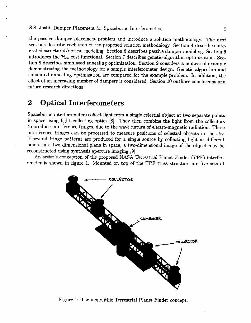
An artist’s conception of the proposed NASA Terrestrial Planet Finder (TPF) interferometer is shown in figure 1. Mounted on top of the TPF truss structure are five sets of

bc 3 0 R

Figure 1: The monolithic Terrestrial Planet Finder concept.


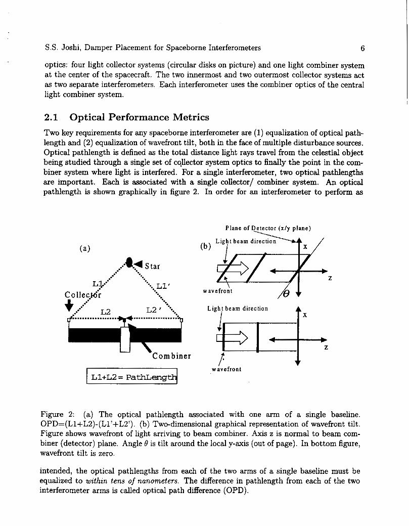
optics: four light collector systems (circular disks on picture) and one light combiner system at the center of the spacecraft. The two innermost and two outermost collector systems act as two separate interferometers. Each interferometer uses the combiner optics of the central light combiner system.

2.1 Optical Performance Metrics Two key requirements for any spaceborne interferometer are (1) equalization of optical pathlength and (2) equalization of wavefront tilt, both in the face of multiple disturbance sources. Optical pathlength is defined as the total distance light rays travel from the celestial object being studied through a single set of cqllector system optics to finally the point in the combiner system where light is interfered. For a single interferometer, two optical pathlengths axe important. Each is associated with a single collector/ combiner system. An optical pathlength is shown graphically in figure 2. In order for an interferometer to perform as

Plane of Detector (x/y plane) "...

f **** *.** L2 L2 ' *=.*

.** t f

e................. ~........'......... *%

u \ Corn biner

-... -*."Z

(b) j Light beam direction "tx /

w avefront $FfZ Light beam direction

1

w avefront

Figure 2: (a) The optical pathlength associated with one arm of a single baseline. OPD=(Ll+L2)-(Ll'+L2'). (b) Two-dimensional graphical representation of wavefront tilt. Figure shows wavefront of light arriving to beam combiner. Axis z is normal to beam combiner (detector) plane. Angle 8 is tilt around the local y-axis (out of page). In bottom figure, wavefront tilt is zero.

intended, the optical pathlengths from each of the two arms of a single baseline must be equalized to within tens of nanometers. The difference in pathlength from each of the two interferometer arms is called optical path difference (OPD).


Disturbance Sources Type Attitude Control Actuators Localized

Delay-line Reaction Localized Siderostat Reaction Localized

Thermal Expansion/Contraction Distributed Microdynamic Distributed

7

Table 1: Typical disturbance sources for optical interferometers. Localized disturbance sources can be traced to a specific location on the interferometer, while distributed sources exert influence over a wide region.

Wavefront tilt is defined as the angle a beam cross-section cuts with respect to a detector- based coordinate system. In order for interference fringes to be uncorrupted, the wavefront tilts of the two beams to be interfered must be equal. Wavefront tilt (WFT) is shown graphically in figure 2 for tilt around the detector-local y axis. Tilt can also be computed for the detector-local x axis. Interferometers are concerned with total tilt defined as WFzotd = ,/WFT,2 + WFT’. The difference in wavefront tilts from each of the two arms of the interferometer is called wavefront tilt difference (WFD).

A

2.2 Disturbance Sources There are several disturbance sources on a spaceborne interferometer that will cause both pathlength difference and tilt. The characterization of all disturbances is an ongoing effort. Some of the most significant sources are listed in table 1. Localized disturbance sources can be traced to a specific location on the interferometer, while distributed sources exert influence over a wide region. In this paper, we focus on sources of disturbance that are ZocaZzzed. We assume reaction wheel disturbances applied to the spacecraft bus and delay-line disturbance forces applied at the locations of the controlled-delay line trolley. Distributed sources of disturbance may be modeled as perturbations of several or all truss joint locations.

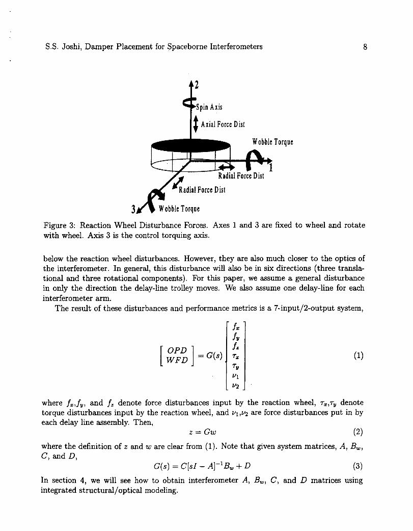
As a reaction wheel spins to provide attitude control authority, it also imparts unwanted disturbance forces and torques to the spacecraft. These unwanted forces and torques are caused by static and dynamic imbalances in the wheel, as well as ball-bearing imperfections and electronics noise [lo]. The nature of reaction wheel disturbances change as the rotation speed of the wheel changes. In practice, five disturbances are modeled for each wheel used in the attitude control system (in reaction wheel local coordinates): one axial force disturbance, two radial force disturbances, and two wobble torque disturbances. These are shown in figure 3. In this paper, we assume a single reaction wheel imparting disturbances in the five directions shown.

Delay-lines consist of a series of optics mounted on moving trolleys. They are used to actively equalize pathlength. The trolleys move in only one direction, parallel to the interferometer truss. However, as they move along their tracks, they also impart mechanical disturbances into the system. The exact nature of the disturbances is still under investi- gation. Preliminary results suggest that these disturbances are several orders of magnitude


d' Spin A x i s

I t Axia l Force D ist

Wobble Torque

p.i Radia l Force D ist

&dial Force Dist

3 J ) Wobble Torque

Figure 3: Reaction Wheel Disturbance Forces. Axes 1 and 3 are fixed to wheel and rotate with wheel. Axis 3 is the control torquing axis.

below the reaction wheel disturbances. However, they are also much closer to the optics of the interferometer. In general, this disturbance will also be in six directions (three transla- tional and three rotational components). For this paper, we assume a general disturbance in only the direction the delay-line trolley moves. We also assume one delay-line for each interferometer arm.

The result of these disturbances and performance metrics is a 7-input/%output system,

OPD [ W F D

where fi,fv, and f z denote force disturbances input by the reaction wheel, T = , T ~ denote torque disturbances input by the reaction wheel, and v1,v2 are force disturbances put in by each delay line assembly. Then,

z = G w (2)

In section 4, we will see how to obtain interferometer A, Bw, C , and D matrices using integrated structural/optical modeling.


3 Interferometer Damper Placement Problem and So- lution Methodology

Assume that there exists only a discrete number of possible locations that a passive damper may be placed. Index every possible location with consecutive integers. This indexed set of locations is given by the integer set P.

Problem

Given:

0 interferometer system architecture

0 number of passive dampers to be placed,K (fixed), and indexed set of possible damper locations,P

Find:

0 optimal locations for K dampers, p* = [pi, pa . . . p x ] with pt E P A

Solution

The methodology we propose to solve this problem is composed of four steps:

1. Develop accurate linear model of interferometer using integrated structural/optical modeling: G( s ) .

2. Model passive dampers within interferometer: G(s,p).

3. Express cost functional ,7 in terms of ?-tm norm.

4. Employ genetic algorithm or simulated annealing optimization to determine optimal damper locations, p'. I

The next sections will describe each step in this.process.

4 Integrated Structural/Optical Modeling A linear integrated model of a spaceborne interferometer consists of a structural model and an optics model that are coupled. We apply finite-element structural modeling to our problem. Finite-element models describe how external forces lead to small displacement and small angle motion at specified points within the structural system. Similarly, differential ray tracing methods use basic reflection and refraction properties of optical elements to ascertain the effects of small displacement and small angle motion of the optical elements on ray position, direction, and length. The common interface between the two models is nodal location. Finite-element structural models transform external forces to nodal movement; linear optical models transform nodal movement to optical path difference and wavefront


tilt. In anticipation of the many applications for integrated models, JPL has developed a number of in-house software tools to aid development of integrated FEM/optics models. These include the Integrated Modeling of Optical Systems (IMOS)[11] and Controlled Optics Modeling Package (COMP) [12] software packages.

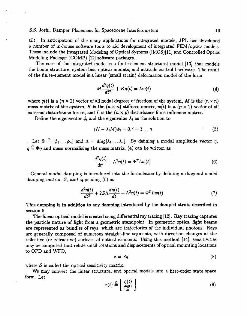
The core of the integrated model is a finite-element structural model [13] that models the boom structure, system bus, optical mounts, and attitude control hardware. The result of the finite-element model is a linear (small strain) deformation model of the form

M - + Kq(t) = Lw(t) &(t> dt2 .

where q(t) is a (n x 1) vector of all nodal degrees of freedom of the system, M is the (n x n) mass matrix of the system, K is the (n x n) stiffness matrix, w(t) is a 0, x 1) vector of all external disturbance forces, and L is the (n x p ) disturbance force influence matrix.

Define the eigenvector & and the eigenvalue Xi as the solution to

( K - X,M)& = 0, i = 1 . . . n (5)

. Let Qi = [@I . . . &J and A = dzag[Al. . . X,]. By defining a modal amplitude vector 7, q = 'Pq and mass normalizing the mass matrix, (4) can be written as

A

A

" @ ) + A2q(t) = @Lw(t) dt2

. General modal damping matrix,

damping is introduced into the formulation by defining a diagonal modal 2, and appending (6) as

This damping is in addition to any damping introduced by the damped struts described in section 5.

The linear optical model is created using differentihl ray tracing (121. Ray tracing captures the particle nature of light from a geometric standpoint. In geometric optics, light beams are represented as bundles of rays, which are trajectories of the individual photons. Rays are generally composed of numerous straight-line segments, with direction changes at the reflective (or refractive) surfaces of optical elements. Using this method [14], sensitivities may be computed that relate small rotations and displacements of optical mounting locations to OPD and WFD,

z =sq where S is called the optical sensitivity matrix.

We may convert the linear structural and optical form. Let

(8)

models into a first-order state space

(9)


Then

" dz(t ) - Az(t) + B,w(t) dt

where

cdq 0 1 D = O . In order to obtain optical outputs,

11

where C = sed. Once the state-space system, A, B,, C, D , is defined, we may create a system transfer function matrix of the form, G(s) = C[sI - A]"B,.

a

5 Passive Damper Modeling Passive dampers are incorporated into the FEM model as viscous dampers based on the Honeywell 'D-strut' [15] concept. A viscous damping force is created along the axial direction that is proportional to the axial displacement rate of an individual strut's beam element. In this article, it is assumed that the new passive damping element and the original truss beam element have the same stiffness, although significant advantage can be gained by optimizing these parameters as well [5]. A new model with a passive damping element, denoted by the subscript i , is written as (in physical coordinates)

where ri is the influence vector associated with an axial force between two nodes of the structure, 6, is a damper actuator force as in [5], and Aki is the change in stiffness associated with the change in elastic modulus of the damper beam element. The force Si is modeled as a linear velocity feedback so

where c, is a scalar parameter used to change the value of damping. Recall in this report, Aki = 0. By substituting (16) into (15), we obtain a damping matrix, V , A

where V E,",, &rir;. Using this formulation, (17) can replace (4).

S.S. -Joshi, Damper Placement for Spaceborne Interferometers

6 3.1, Cost Functional Using the state space description of the system (10-14), we obtained

" dz(t ) - A z ( t ) + B,w(t) d t

12

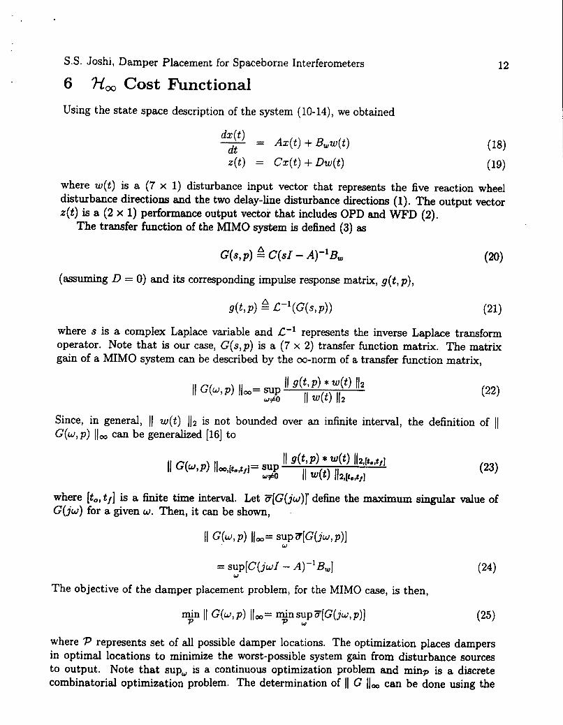
Z ( t ) = Cz(t) + Dw(t) (19) where w(t ) is a (7 X 1) disturbance input vector that represents the five reaction wheel disturbance directions and the two delay-line disturbance directions (1). The output vector ~ ( t ) is a (2 x 1) performance output vector that includes OPD and WFD (2).

The transfer function of the MIMO system is defined (3) as

(assuming D = 0) and its corresponding impulse response matrix, g ( t , p ) ,

where s is a complex Laplace variable and represents the inverse Laplace transform operator. Note that is our case, G(s,p) is a (7 x 2) transfer function matrix. The matrix gain of a MIMO system can be described by the ,-norm of a transfer function matrix,

11 w(t ) 112 is not bounded over an infinite interval, the definition of 11 generalized [lS] to

where [to, t f ] is a finite time interval. Let a[G(jw)T d e h e the maximum singular value of G(jw) for a given w. Then, it can be shown, .

= SUP[C(~WI - A)"&] (24) W

The objective of the damper placement problem, for the MIMO case, is then,

where P represents set of all possible damper locations. The optimization places dampers in optimal locations to minimize the worst-possible system gain from disturbance sources to output. Note that sup, is a continuous optimization problem and minp is a discrete combinatorial optimization problem. The determination of 11 G 1100 can be done using the

S.S. .Joshi, Damper Placement for Spaceborne Interferometers 13

nonnhinflm) function in MATLAB, which uses a binary search algorithm for optimization

For systems with dissimilar inputs and/or outputs, weighting matrices can be incorporated into the optimization cost function. In this way, the solution is not skewed by inputs or outputs that differ in magnitude solely because of units. For the interferometer case, this is important as OPD has units of meters and WFD has units of radians. In addition, reaction wheel disturbances and delay-line disturbances may have very different magnitudes. Therefore, we define two (2 x 2) weighting matrices, Wo and W,. Then the optimization problem (25) is modified as

[171.

min 11 WoG(u,p)Wi l l o o P (26) Wo is used to weight the perforrriance output and Wi is used to weight the disturbance inputs. Since we would like OPD and WFD to have comparable effects on the optimization problem, we select 7 such that

I I G ~ + O P D Ilm= Y I I G - W F D ll, (27)

where G w - , ~ p D and G w - , w ~ ~ are (7 x 1) transfer function matrices to a single output with only modal damping (zero passive dumper elements). Then

Less is known about relative magnitudes of localized interferometer disturbance sources. Therefore, an identity matrix is chosen for Wi. This choice has two interpretations: (1) delay-line disturbances have the same relative effect on the ‘H, norm as the reaction wheel disturbances (unlikely) or (2) the disturbances have been preweighted before being applied. Note that, in general, the weighting matrices W o ( j w ) and W,( jw) can be functions of frequency. As more is learned about the relative nature of disturbances, a frequency-shaped weighting matrix may be more appropriate.

7 Genetic Algorithm Optimization In the past decade, powerful new heuristic optimization techniques have developed based on the biological processes of evolution, adaptation, and survival of the fittest. These methods are broadly defined under the term “evolutionary programs.” One popular algorithm used in optimization is the genetic algorithm (GA). Unlike other popular heuristic optimization techniques (such as simulated annealing) GA methods maintain a fami ly of solutions, called a population, at every iteration. Between iterations, the members of each population, called chromosomes, interact with each other to form a new population. Every new population is called a generation. Eventually, with enough generations, a near-optimal solution is obtained. The theoretical foundation of GA methods lie in the computer science notion of a schema (181. Note however, like other heuristic optimization techniques, optimally is not guaranteed. We implement a GA method based on seven common steps [ M I : (1) binary representation of chromosomes, (2) random selection of initial population, (3) selection of fittest chromosomes, (4) crossover, (5) mutation, ( 6 ) chromosome repair, and (7) evaluation.


Representation of Chromosomes

An individual chromosome represents a possible solution to the damper placement problem. First, all possible damper locations are ordered and assigned an integer label, 1 . . . N . Each label is then represented in binary form. For example location “94” is “1011110”. The binary locations are appended to form a single chromosome. For example, if three dampers are to be placed, a possible solution is [8 34 911. This means one damper is placed at location 8, one at location 34, and finally one at location 91. The chromosome associated with this solution is [OOOlOOOOlOOOlOlOllOllJ . Leading zeros are added so each binary location is represented by the same number of bits. Since the number of dampers to be placed , X , remains fixed, the length of each chromosome also remains f i x e d .

Random Selection of Initial Population

The size, sp, of a population determines the number of chromosomes that make up a population. For an initial population, solutions are created at random. For the damper placement problem, a restriction is imposed that only one damper may be placed at any given location.

Selection of Fittest Chromosomes

Given a population, each chromosome may be evaluated for its fitness. In our case, the fittest chromosome is one with the lowest 11 W,GWi /loo (26) cost, denoted J( i ) . From a given population, a new population is created by the following selection process:

0 Calculate total fitness of a population, 3, defined as 3 fi xi”,, J ( i )

0 Calculate a probability, e, for each chromosome, e = J( i ) /F

0 Calculate a cumulative probability, qi, for each chromosome, qi 2 e( i )

0 Generate sp random floats, +(z), from [0,1]

A

. I

If $(i) < q1, then select chromosome 1; else select ,the ith chromosome such that Qi-1 < +(i) < Qt

Note that with this process, some chromosomes will be selected more than once. In the end, the total size of the new population will remain sp.

Crossover

Given the new selected population, it is now modified using the crossover operation. Crossover can be thought of as the mating of two chromosomes to create children chromosomes. First, a probability of crossover, PC, is defined. This is the probability that any given chromosome within a population will be chosen for crossover. Then, for each chromosome in the population,


e Generate a random float, $(z), from [0,1]

e If $(i) < PC, then select chromosome for crosmver

e Pair up all selected chromosomes. If number of selected chromosomes is not even, randomly add another from the population

e Generate a random integer, pos, for each pair. This is the crossover point within a chromosome pair

0 Perform crossover for each pair; i.e. replace (ala2 , . . t+%+1. . . and (bib . . . bmbm+l . . . b with ( a l e . . .+&+I.. . bm) and (bib.. . b m ~ + a + l . . . om)

This operation creates yet another intermediate population.

Mutation

Mutation is another operation to create an additional intermediate population. This operation occurs on each bit within each chromosome of a population. First, define a probability of mutation, p m . Then for each bit,

e Generate a random float, +(i), from [OJ]

If +(i) < p m , then select bit for mutation

For each selected bit, if it is 0, change to 1 and vise versa.

Typically, the probability of mutation, p m , is much lower than the probability of crossover, PC. This operation creates one more intermediate population.

Chromosome Repair

Given the selection, crossover, and mutation operators, a new population arises. However, this population was not subject to any practical conitrainis. For instance, a chromosome in the new population could generate damper locations than are greater than n/. In addition, chromosomes may appear with repeated damper locations. There are many ways to handle such a situation. One could proceed with the infeasible solutions and heavily penalize the chromosomes in the selection phase. In this way, the chromosomes would not survive in the selection step. This is sometimes referred to as the “death penalty”. Another way to proceed is to repair the infeasible solutions. In this work, we identify the chromosomes with infeasible damper locations and then replace them with the best chromosome of the previous generation. This repaired population becomes a generation.

Generation Evaluation

Given the final repaired population, each chromosome is evaluated and its best solution is identified. The process then continues with the Selection of Fittest Chromosomes step.

S.S. ,Joshi, Damper Placement for Spaceborne Interferometers 16

8 Simulated Annealing (SA) Simulated annealing has previously been used for discrete optimization in damper placement problems by [5] and [4]. Therefore, it is not discussed in as much detail as Genetic Algorithms. Most common combinatorial optimization routines follow an iterative improvement strategy in which a trial solution cost is compared to the previous low combination cost. If the new cost is lower, then the trial solution is deemed the new low-cost combination. This method will find local minima, but has the disadvantage of being stuck in a particular local minimum even though other local minima may provide a lower overall cost. The simulated annealing strategy differs in that is occasionally accepts a trial solution as the new low-cost solution even though the new cost has actually increased. This occasional acceptance of a non-improving trial combination allows'the current solution to jump to other local minima. The probability of accepting a non-improving solution is governed by a so called Boltzmann probability function

B p = ,-AJ/P (29) where AJ' is the change in cost from the previous low-cost combination and p is a free- parameter known as the pseudo-temperature. p is slowly decreased as the algorithm pro- ceeds. It is to be noted that as the temperature decreases, the probability of accepting a non-improving solution also decreases. This forms a convergence pattern in which initially many non-improving solutions are accepted resulting in increased overall cost, but eventually the search settles to a particular local minimum region where only lower cost combinations are accepted. Note also that large increases in 3 (large positive AJ), prohibit the acceptance of a non-improving trial combination. In the simulated annealing routine we implemented, a new trial combination is created by perturbing one element in the current low-cost combination. The element which is perturbed is selected by a uniform random number generator. This element is changed to a random value in the space of all possible damper locations again by a uniform random number generator.

9 Numerical Example

9.1 Example Interferometer Description Consider a model of a free-flying, 10 meter baseline, dual-star feed interferometer. The model includes two trusses on which collecting apertures are mounted, a rigid central bus node modeled after the NASA Space Shuttle ASTRO-SPAS carrier, and attachment points for the optical elements. The ASTRO-SPAS bus node is connected to an optics node via a rigid body element. The two trusses are composed af interlocking six-degree-of-freedom beam elements. The ASTRO-SPAS bus node is connected to the trusses by four rigid body elements to each of the four corners of each truss. The geometry of the interferometer structure and disturbance input locations are shown in figure 4.

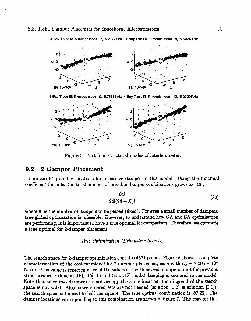
The length of each of the two trusses is 4 meters. It is partitioned into 4 one-meter long bays. The cross section of each bay is 0.28 x 0.28 m2. Each truss is composed of 57 IMOS beam elements [ll]. The first four non rigid-body modes of the interferometer structure are shown in figure 5.

S.S. Joshi, Damper Placement For Spaceborne Interferometers

4-Bay Truss Interferometer Model

17

Figure 4: Representative Interferometer. Reaction wheel disturbances are input at the bus. Delay line disturbances are input on the trusses.

From the double truss interferometer model, standard mass and stiffness matrices associated with a finite-element model were obtained. The model contained 408 degrees of freedom in physical coordinates. This resulted in physical-coordinate mass, M , and stiffness, K , matrices E 7EaXao8. Of the 408 degrees of freedom, several were dependent DOF's. The dependent degrees of freedom were due to rigid body element connections. After re- moving these dependent degrees of freedom, 162 degrees of freedom remained, resulting in reduced mass and stif€ness matrices, Mr and K,, E 7Z162x162. This model was still too large to be analyzed repeatedly. As a result, the model was truncated. A transformation matrix,

E 7Z162x50 was composed of 50 eigenvectors,

where [dl, 4 2 , . . . , 461 were the rigid-body modes. A reduced order system was then produced as

where W M Q , E R50x50, a t K @ E and QtL E R50 . Before arriving at the interference point, light rays trace a path through several optical

elements including siderostats, beam compressors, and steering mirrors [8]. This defines an optical sensitivity matrix S .


4-Bay Truss lSlS model: mode 7. 5.23777 Hz 4-Bay Truss lSlS model: mode 8, 5.60243 Hz

18

4-Bay TNSS lSlS m o d e l : mode 9, 5.76158 Hz 4-Bay Truss lSlS model: mode 10, 6.23295 Hz

Figure 5: First four structural modes of interferometer.

9.2 2 Damper Placement There are 94 possible locations for a passive damper in this model. Using the binomial coefficient formula, the total number of possible damper combinations grows as [19],

94! 94!(94 - X ) !

where K: is the number of dampers to be placed (fixed). For even a small number of dampers, true global optimization is infeasible. However, to understand how GA and SA optimization are performing, it is important to have a true optimal for comparison. Therefore, we compute a true optimal for 2-damper placement.

True Optimization (Exhaustive Search)

The search space for 2-damper optimization contains 4371 points. Figure 6 shows a complete characterization of the cost functional for 2-damper placement, each with c, = 7.005 x lo4 Ns/m. This value is representative of the values of the Honeywell dampers built for previous structures work done at JPL (151. In addition, .l% modal damping is assumed in the model. Note that since two dampers cannot occupy the same location, the diagonal of the search space is not valid. Also, since ordered sets are not needed (solution [1,2] solution [2,1]), the search space is limited to half the square. The true optimal combination is [87,22]. The damper locations corresponding to this combination are shown in figure 7. The cost for this


Map d 2-Damper Cost Functional

19

1 0 2 0 3 0 4 0 5 0 6 0 7 0 8 0 9 3 Damper Position 1

Figure 6: Cost functional, 3, as a function of two damper locations. Blue color is low cost (good) and red color is high cost (bad). The optimal location is [87,22].

Population Size (sp) 10 Probability of Crossover ( P C )

0.02 Probability of Mutation (pm) 0.40

Number of Generations 48

Table 2: Parameters chosen for GA optimization.

optimal is 3 = 2.21e - 3. For 2 dampers, this exhaustive search took 24.3 hours on a SUN UltraSparc 20, or approximately 20 seconds per cost evaluation. For just 3 dampers, an exhaustive search would take over 31 days.

In the following sections. we compare both performance and runtime for 2-damper o p timization using both the GA and SA optimization method. Runtime is dominated by the evaluation of the cost functional, 3. Therefore, the runtime is defined in terms of the number of times the cost functional is evaluated.

GA Optimization

The same 2-damper optinlization is now perforwed using the GA. The relevant parameters for the GA are shown in table 2. Figures (8) shows a representative GA optimization search pattern for the optimal placement of two clanlpers, each with c, = 7.005 X lo4 Ns/m



20

Y

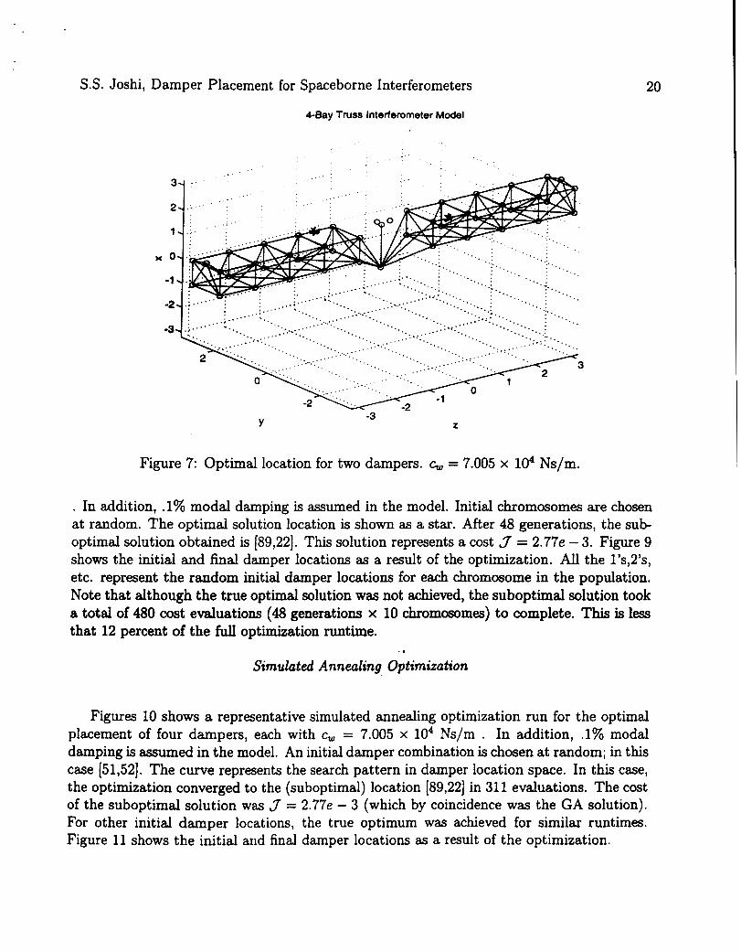
Figure 7: Optimal location for two dampers. c, = 7.005 x lo4 Ns/m.

. In addition, .l% modal damping is assumed in the model. Initial chromosomes are chosen at random. The optimal solution location is shown as a star. After 48 generations, the suboptimal solution obtained is [89,22]. This solution represents a cost J = 2.77e - 3. Figure 9 shows the initial and final damper locations as a result of the optimization. All the l’s,2’s, etc. represent the random initial damper locations for each chromosome in the population. Note that although the true optimal solution was not achieved, the suboptimal solution took a total of 480 cost evaluations (48 generations x 10 chromosomes) to complete. This is less that 12 percent of the full optimization runtime.

.. Simulated Annealing Optimization

Figures 10 shows a representative simulated annealing optimization run for the optimal placement of four dampers, each with c, = 7.005 x lo4 Ns/m . In addition, .l% modal damping is assumed in the model. An initial damper combination is chosen at random; in this case (51,521. The curve represents the search pattern in damper location space. In this case, the optimization converged to the (suboptimal) location (89,221 in 311 evaluations. The cost of the suboptimal solution was 3 = 2.77e - 3 (which by coincidence was the GA solution). For other initial damper locations, the true optimum was achieved for similar runtimes. Figure 11 shows the initial and final damper locations as a result of the optimization.


90-

80-

70 -

GA Search

.6'

:* 00 0 0

:* 0 e o 0

21

Figure 8: GA Optimization Search Pattern: 2 Dampers. The circles on the lower right triangle show the locations checked; the star represents the true optimal solution.

9.3 Comparison of GA and SA algorithms Several observations result from comparing the two optimization schemes. First, both algorithms obtain (suboptimal), but excellent solutions in a fraction of the runtime needed for true optimization. Indeed, true optimization is essentially impossible for anything more than 2 dampers. However, the SA algorithm outperformed the GA algorithm for this problem. The quality of both solutions was excellent. However, the SA algorithm was about twice as fast in obtaining a solution. In particular, the SA algorithm benefited from an observed "slot machine" effect. Once a.n optimal damper location was achieved for a single damper, this element of the solution combination was rarely changa. Instead, it was locked in place while other dampers were optimally placed. In this way, the optimization proceeded in almost a damper by damper succession. This was not the case with GA optimization, as crossover and mutation produced different damper locations at each iteration. Both optimization methods depend very much on governing parameters. We found that the SA routine regularly converged to a single solution. Convergence was harder to establish for the GA routine. This will especially be true in the usual case where the true optimum is unknown. One rule of thumb we found helpful was the evaluation of total fitness, 3, for each generation. Total fitness climbed (on average) for a certain amount of iterations, and then stabilized. The overall best solution for the GA optimization occurred first at the point of total fitness stabilization.



22

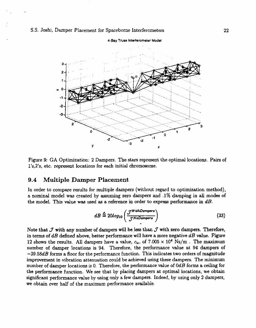
Figure 9: GA Optimization: 2 Dampers. The stars represent the optimal locations. Pairs of l’s,2’s, etc. represent locations for each initial chromosome.

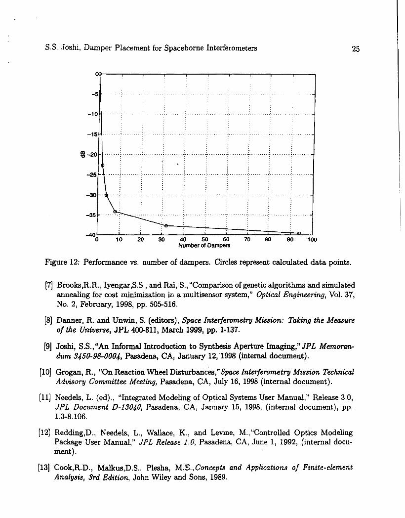
9.4 Multiple Damper Placement In order to compare results for multiple dampers (without regard to optimization method), a nominal model was created by assuming zero dampers and .l% damping in all modes of the model. This value was used as a reference in order to express performance in dB.

*

Note that ,7 with any number of dampers will be,less than 3 with zero dampers. Therefore, in terms of dB defined above, better performance will have a more negative dB d u e . Figure 12 shows the results. All dampers have a value, G, of 7.005 x lo4 Ns/m . The maximum number of damper locations is 94. Therefore, the performance value at 94 dampers of -39.58dB forms a floor for the performance function. This indicates two orders of magnitude improvement in vibration attenuation could be achieved using these dampers. The minimum number of damper locations is 0. Therefore, the performance value of OdB forms a ceiling for the performance function. We see that by placing dampers at optimal locations, we obtain significant performance value by using only a few dampers. Indeed, by using only 2 dampers, we obtain over haif of the maximum performance available.


1 0 2 0 3 0 4 0 5 0 8 0 7 0 8 0 9 0 O l n p S r P ~ l

Figure 10: SA Optimization Search Pattern: 2 Dampers. The circles on the lower right triangle show the locations checked; the star represents the true optimal solution.

10 Conclusions Vibration attenuation will be crucial to next generation space observatories that use interferometry. Damper placement will be a challenging issue for these systems. As new optimization schemes are developed, this process will hopefully become more and more efficient. In this paper, we introduced a general methodology for damper placement in interferometers. This methodology included optical-structural modeling, damper modeling, 3.100 cost functional formulation, and combinatorial optimization. The cost functional based on 811 7-t- norm allows multiple dissimilar disturbance sources and multiple dissimilar performance outputs. Both GA and SA optimization were investigated. Both techniques produced quality solutions. However, the SA algorithm was much more efficient for this problem.

11 Acknowledgments The author would like to acknowledge Dr. Mark Milman of JPL for introducing him to the damper placement problem, and for many helpful discussions. The author would also like to thank Dr. Scott Ploen of JPL for his careful review and constructive comments. This work was performed at the Jet Propulsion Laboratory, under a contract from the National Aeronautics and Space Administration.


4-Bay Truss interferometer Model

Figure 11: SA Optimization: 2 Dampers. The stars represent the find locations. The circles represent the initid locations.

References [l] Melody, J.W. and Neat, G.W., “Integrated Modeling Methodology Validation Using the

MicroPrecision Interferometer Testbed,” Proceedings of the 35th IEEE Conference on Decision and Control, Vo1.4, Kobe, Japan, December, 1996, pp.4222-4227.

[2] Spanos, J.T., Rahman, Z., and Blackwood, G.,“A Soft &Axis Active Vibration Isolator,”

[3] Joshi, S.S., Milman, M., and Melody, J.W.,“Optimal Passive Damper Placement Methodology for Interferometers Using Integrated Structures/Optics Modeling,” A IAA Guidance and Control Conference, New Orleans, LA, August, 1997, pp. 1-8.

[4] Chen, G.-S., Bruno, R. J., and Salama, M., “Optimal Placement of Active/Passive Mem- bers in Truss Structures Using Simulated Annealing,” AIAA Journal, Vol. 29, No. 8,

[5] Milman, M.H. and C.-C. Chu, “Optimization Methods for Passive Damper Placement and Tuning,” Journal of Guidance, Control, and Dynamics, Vol. 17, No. 4, July-August,

(6) Hamernik, T.A., Garcia, E., and Stech, D. “Optimal Placement of Damped Struts Using Simulated Annealing,” Journal of Spacecraft and Rockets, Vol. 32, No. 4, July-August,

American Control Conference, Seattle, WA, June, 1995,pp. 412-416. ..

August, 1991, pp. 1327-1334.

1994, pp. 848-856.

1995, pp. 653-661.

24

S.S. ,Joshi, Damper Placement for Spaceborne Interferometers

op I I 1 1 I I I I I I

I . . . . . . . . . . . . . . . . . . . . . . . . . . . . . . . .

-10 t

. . . . . . . . . . . . . . . . . . . . . . . . . . . . . . . . . . . . . . . . . . . . . . . . . . . . . . . . . . . . . . . . . . . . . . . . . . . . . . . . . . . . . . . . . . . . . . . -I I I i I I I I . . . . . . . . . i . . . . . . . . . : ... . . . . . . 1 . . . . . . . . . L . . . . . . . . . i . . . . . . . . . . i ......... i .. . . . . . . . i . . . . . . . . . i . . . . . . . . i

4 5 ......... ; ......... ; ........ .:. ........ .:. ........ .:. ........ .:. ........ ........ ........

30

25

0 10 20 30 40 50 60 70 80 90 1 0 0 Number of Dampers

Figure 12: Performance v s . number of dampers. Circles represent calculated data points.

[7] Brooks,R.R., Iyengar,S.S., and Rai, S.,“Comparison of genetic algorithms and simulated annealing for cost minimization in a multisensor system,” Optical Engineering, Vol. 37, No. 2, February, 1998, pp. 505516.

[8] Danner, R. and Unwin, S. (editors), Space Interferometry Mission: Taking the Measure of the Universe, JPL 400-811, March 1999, pp. 1-137.

[9] Joshi, S.S., “An Informal Introduction to Synthesis Aperture Imaging,” JPL Memoran- dum 3450-98-0004, Pasadena, CA, January 12,’1998 (internal document).

[lo] Grogan, R., “On Reaction Wheel Disturbanc&,”Space Ivterfervmetry Mission Technical Advisory Committee Meeting, Pasadena, CA, July 16, 1998 (internal document).

[ll] Needels, L. (ed)., “Integrated Modeling of Optical Systems User Manual,” Release 3.0, JPL Document 0-13040, Pasadena, CA, January 15, 1998, (internal document), pp. 1.3-8.106.

(121 Redding,D., Needels, L., Wallace, K., and Levine, M.,“Controlled Optics Modeling Package User Manual,” JPL Release 1.0, Pasadena, CA, June 1, 1992, (internal document).

[13] Cook,R.D., Malkus,D.S., Plesha, M.E.,Concepts and Applications of Finite-element Analysis, 3rd Edition, John Wiley and Sons, 1989.


[14] Redding, D. and Breckenridge, W., “Optical Modeling for Dynamics and Control Anal- ysis,” Journal of Guidance, Control, and Dynamics, Vol. 14, September, 1991, pp. 1021-1032.

[15) Neat, G.W., O’Brien J.F., Lurie, B.J., and Garnica, A.,“Joint Langley Research Center/ JPL CSI Experiment,” 15th Annual AAS Guidance and Control Conference, February 8-12, 1992, pp. 1-7.

[IS] Burl, J.B.,Lineur Optimal Control, Addison-Wesley, Menlo Park, 1999, pp. 101-118.

[17] Chiang, R.Y., and Safanov, M.G., Robust Contml Toolbox for we with MATLAB, The Mathworks, Inc., August 1992, p ~ . 2.84-2.85.

[18] Michalewia, Z. Genetic Algorithms + Data Structum= Evolution Pqqmms, Springer, New York, 1992, pp. 1-94.

[19] Leon-Garcia, A. Probability and Random Processes for Electrical Engineering, Addison- Wesley Publishing Company, New York, 1989, pp. 48-54.

Date post:	21-Oct-2015
Category:	Documents
Upload:	arjun-shende
View:	4 times
Download:	0 times

99-0878

Documents